CHAPTER VIII Data Clustering and Self-Organizing Feature...
13
Ugur HALICI ARTIFICIAL NEURAL NETWORKS CHAPTER 8 EE543 LECTURE NOTES . METU EEE . ANKARA 126 CHAPTER VIII Data Clustering and Self-Organizing Feature Maps Self organizing feature maps (SOFM) - also called Kohonen feature maps - are a special kind of neural networks that can be used for clustering tasks. The goal of clustering is to reduce the amount of data by categorizing or grouping similar data items together. A SOFM consists of two layers of neurons: an input layer and a so-called competition layer. The weights of the connections from the input neurons to a single neuron in the competition layer are interpreted as a reference vector in the input space. That is, a SOFM basically represents a set of vectors in the input space: one vector for each neuron in the competition layer. A SOFM is trained with a method that is called competition learning: When an input pattern is presented to the network, that neuron in the competition layer is determined, the reference vector of which is closest to the input pattern. This neuron is called the winner neuron and it is the focal point of the weight changes. In pure competition only the weights of the connections leading to the winner neuron are changed. The changes are made in such a way that the reference vector represented by these weights is moved closer to the input pattern. In SOFMs, however, not only the weights of the connections to the winner neuron are adapted. Rather, there is a neighborhood relation defined on the competition layer which indicates which weights of other neurons should also be changed. This neighborhood relation is usually represented as a (usually two-dimensional) grid, the vertices of which are the neurons. This grid most often is rectangular or hexagonal. During the learning process, the weights of all neurons in the competition layer that lie within a certain radius around the
-
Upload
dinhkhuong -
Category
Documents
-
view
228 -
download
0
Transcript of CHAPTER VIII Data Clustering and Self-Organizing Feature...
Ugur HALICI ARTIFICIAL NEURAL NETWORKS CHAPTER 8
EE543 LECTURE NOTES . METU EEE . ANKARA
126
CHAPTER VIII
Data Clustering and Self-Organizing Feature Maps
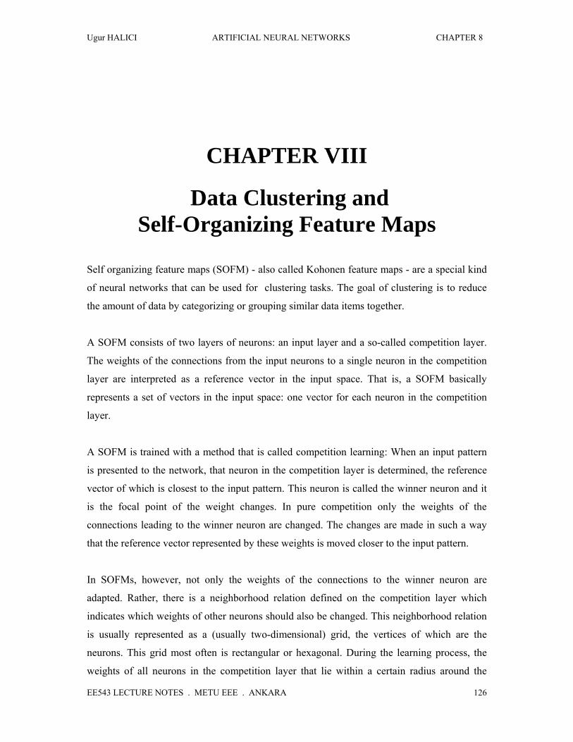
Self organizing feature maps (SOFM) - also called Kohonen feature maps - are a special kind
of neural networks that can be used for clustering tasks. The goal of clustering is to reduce
the amount of data by categorizing or grouping similar data items together.
A SOFM consists of two layers of neurons: an input layer and a so-called competition layer.
The weights of the connections from the input neurons to a single neuron in the competition
layer are interpreted as a reference vector in the input space. That is, a SOFM basically
represents a set of vectors in the input space: one vector for each neuron in the competition
layer.
A SOFM is trained with a method that is called competition learning: When an input pattern
is presented to the network, that neuron in the competition layer is determined, the reference
vector of which is closest to the input pattern. This neuron is called the winner neuron and it
is the focal point of the weight changes. In pure competition only the weights of the
connections leading to the winner neuron are changed. The changes are made in such a way
that the reference vector represented by these weights is moved closer to the input pattern.
In SOFMs, however, not only the weights of the connections to the winner neuron are
adapted. Rather, there is a neighborhood relation defined on the competition layer which
indicates which weights of other neurons should also be changed. This neighborhood relation
is usually represented as a (usually two-dimensional) grid, the vertices of which are the
neurons. This grid most often is rectangular or hexagonal. During the learning process, the
weights of all neurons in the competition layer that lie within a certain radius around the
Ugur HALICI ARTIFICIAL NEURAL NETWORKS CHAPTER 8
EE543 LECTURE NOTES . METU EEE . ANKARA
127
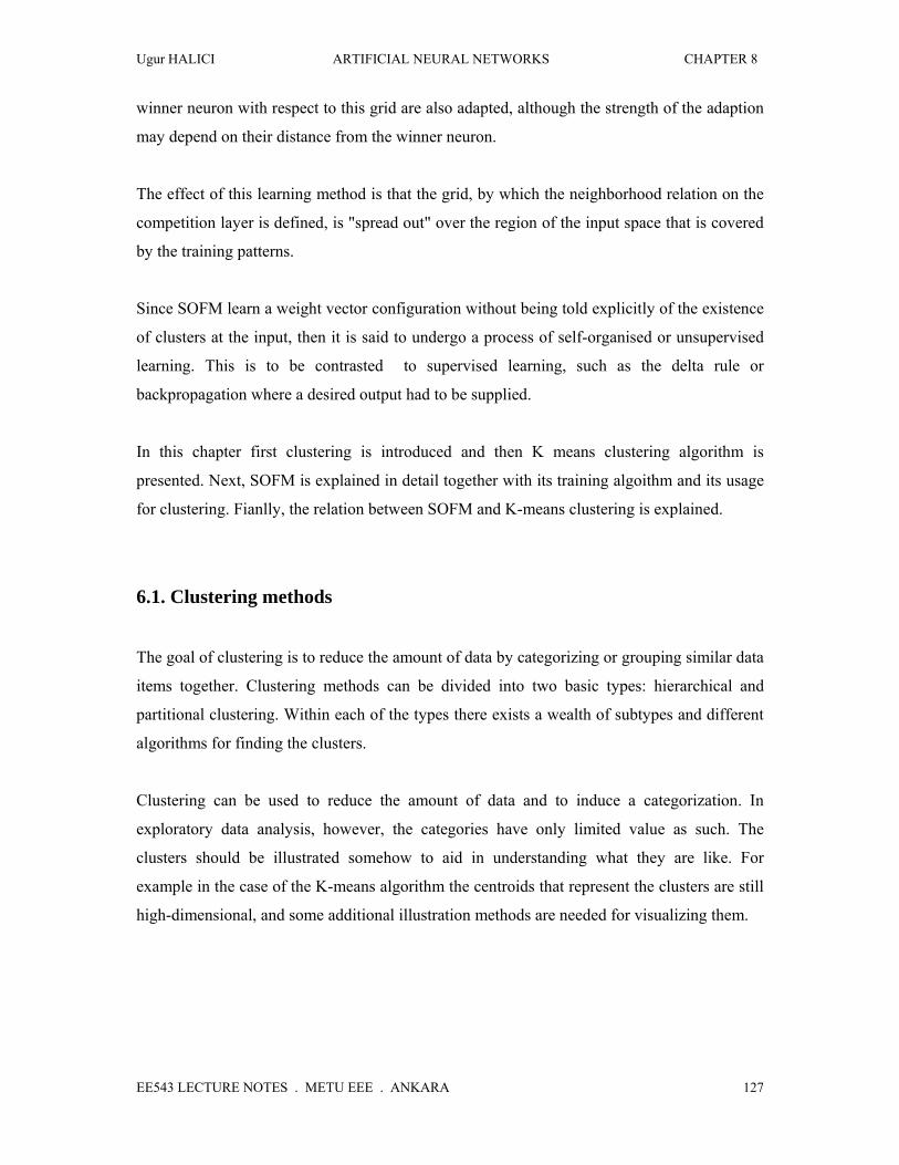
winner neuron with respect to this grid are also adapted, although the strength of the adaption
may depend on their distance from the winner neuron.
The effect of this learning method is that the grid, by which the neighborhood relation on the
competition layer is defined, is "spread out" over the region of the input space that is covered
by the training patterns.
Since SOFM learn a weight vector configuration without being told explicitly of the existence
of clusters at the input, then it is said to undergo a process of self-organised or unsupervised
learning. This is to be contrasted to supervised learning, such as the delta rule or
backpropagation where a desired output had to be supplied.
In this chapter first clustering is introduced and then K means clustering algorithm is
presented. Next, SOFM is explained in detail together with its training algoithm and its usage
for clustering. Fianlly, the relation between SOFM and K-means clustering is explained.
6.1. Clustering methods
The goal of clustering is to reduce the amount of data by categorizing or grouping similar data
items together. Clustering methods can be divided into two basic types: hierarchical and
partitional clustering. Within each of the types there exists a wealth of subtypes and different
algorithms for finding the clusters.
Clustering can be used to reduce the amount of data and to induce a categorization. In
exploratory data analysis, however, the categories have only limited value as such. The
clusters should be illustrated somehow to aid in understanding what they are like. For
example in the case of the K-means algorithm the centroids that represent the clusters are still
high-dimensional, and some additional illustration methods are needed for visualizing them.
Ugur HALICI ARTIFICIAL NEURAL NETWORKS CHAPTER 8
EE543 LECTURE NOTES . METU EEE . ANKARA
128
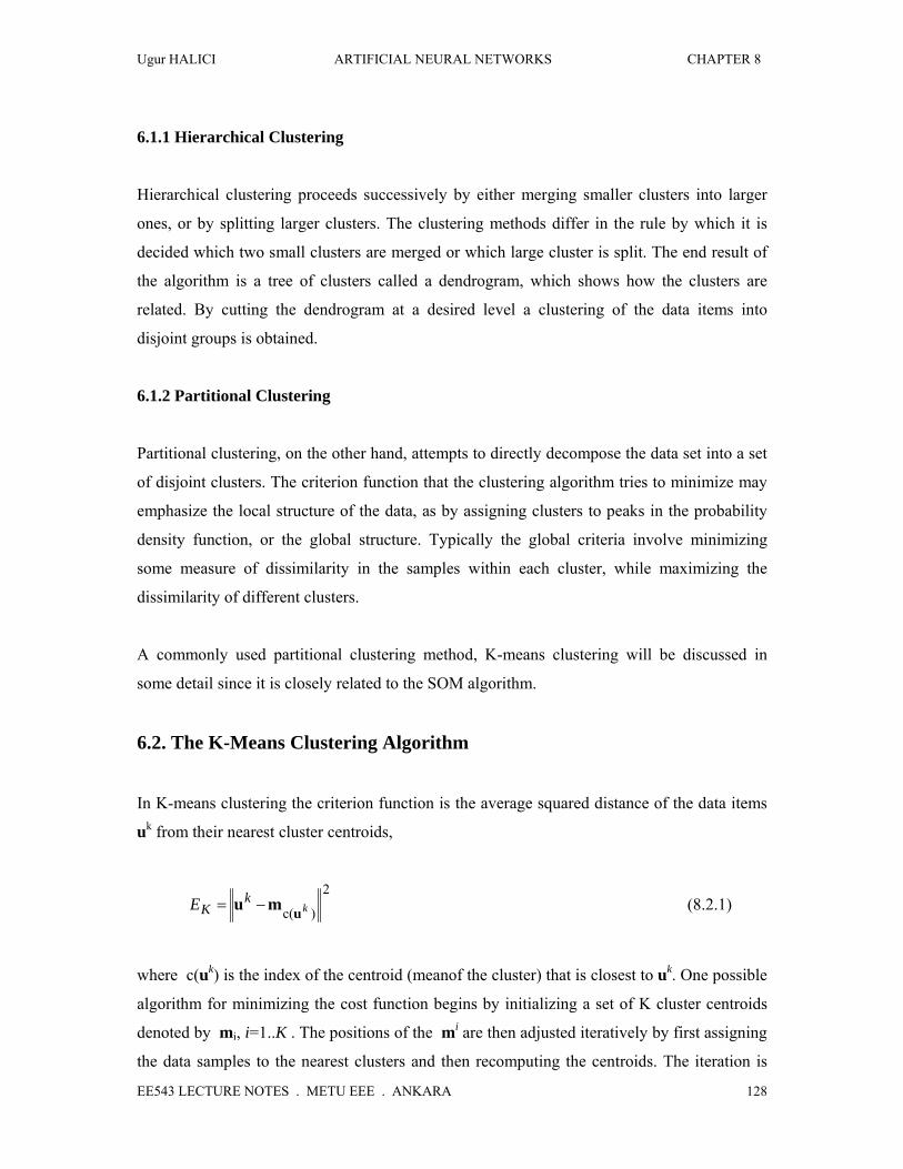
6.1.1 Hierarchical Clustering
Hierarchical clustering proceeds successively by either merging smaller clusters into larger
ones, or by splitting larger clusters. The clustering methods differ in the rule by which it is
decided which two small clusters are merged or which large cluster is split. The end result of
the algorithm is a tree of clusters called a dendrogram, which shows how the clusters are
related. By cutting the dendrogram at a desired level a clustering of the data items into
disjoint groups is obtained.
6.1.2 Partitional Clustering
Partitional clustering, on the other hand, attempts to directly decompose the data set into a set
of disjoint clusters. The criterion function that the clustering algorithm tries to minimize may
emphasize the local structure of the data, as by assigning clusters to peaks in the probability
density function, or the global structure. Typically the global criteria involve minimizing
some measure of dissimilarity in the samples within each cluster, while maximizing the
dissimilarity of different clusters.
A commonly used partitional clustering method, K-means clustering will be discussed in
some detail since it is closely related to the SOM algorithm.
6.2. The K-Means Clustering Algorithm
In K-means clustering the criterion function is the average squared distance of the data items
uk from their nearest cluster centroids,
2
)c( kk
KE umu −= (8.2.1)
where c(uk) is the index of the centroid (meanof the cluster) that is closest to uk. One possible
algorithm for minimizing the cost function begins by initializing a set of K cluster centroids
denoted by mi, i=1..K . The positions of the mi are then adjusted iteratively by first assigning
the data samples to the nearest clusters and then recomputing the centroids. The iteration is
Ugur HALICI ARTIFICIAL NEURAL NETWORKS CHAPTER 8
EE543 LECTURE NOTES . METU EEE . ANKARA
129
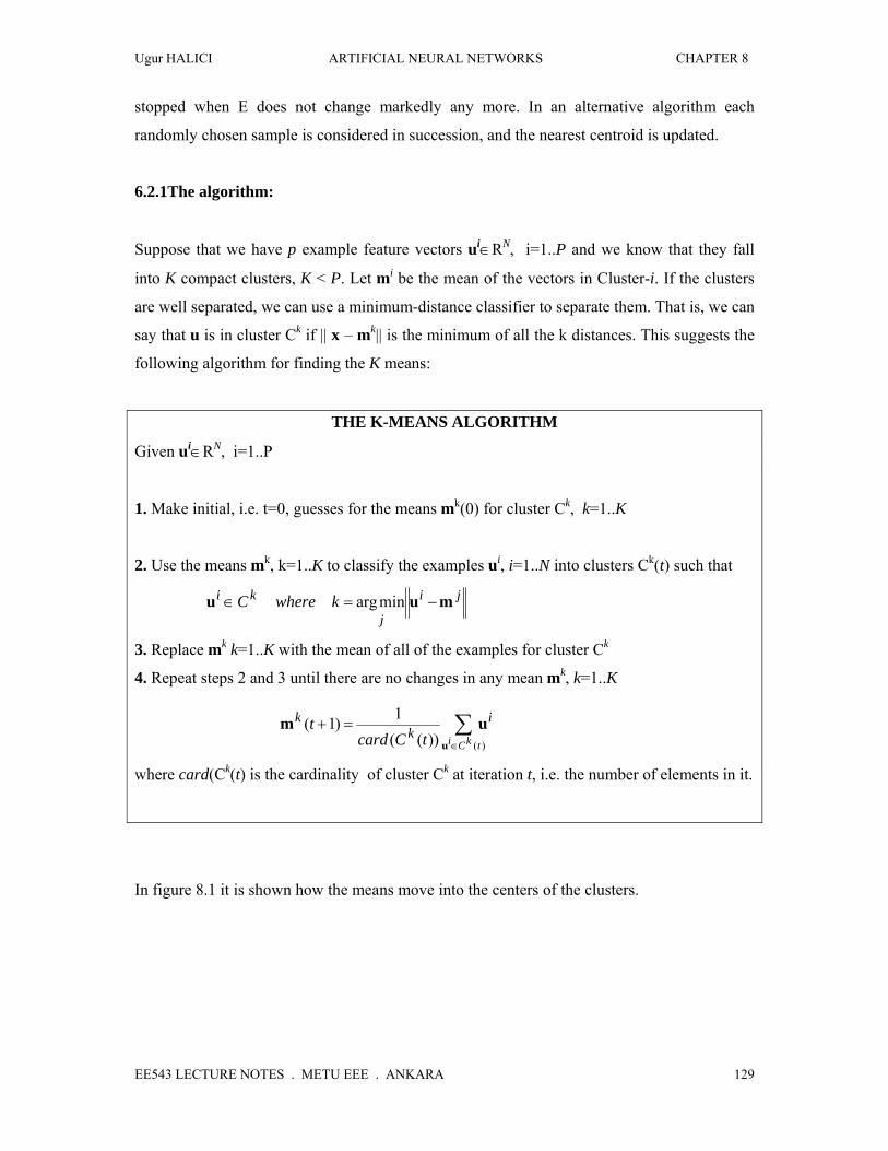
stopped when E does not change markedly any more. In an alternative algorithm each
randomly chosen sample is considered in succession, and the nearest centroid is updated.
6.2.1The algorithm:
Suppose that we have p example feature vectors ui∈RN, i=1..P and we know that they fall
into K compact clusters, K < P. Let mi be the mean of the vectors in Cluster-i. If the clusters
are well separated, we can use a minimum-distance classifier to separate them. That is, we can
say that u is in cluster Ck if || x – mk|| is the minimum of all the k distances. This suggests the
following algorithm for finding the K means:
THE K-MEANS ALGORITHM
Given ui∈RN, i=1..P
1. Make initial, i.e. t=0, guesses for the means mk(0) for cluster Ck, k=1..K
2. Use the means mk, k=1..K to classify the examples ui, i=1..N into clusters Ck(t) such that
ji
j
ki kwhereC muu −=∈ minarg
3. Replace mk k=1..K with the mean of all of the examples for cluster Ck
4. Repeat steps 2 and 3 until there are no changes in any mean mk, k=1..K
∑∈
=+)())((
1)1(tkCi
ik
k
tCcardt
u
um
where card(Ck(t) is the cardinality of cluster Ck at iteration t, i.e. the number of elements in it.
In figure 8.1 it is shown how the means move into the centers of the clusters.

Ugur HALICI ARTIFICIAL NEURAL NETWORKS CHAPTER 8
EE543 LECTURE NOTES . METU EEE . ANKARA
130
Figure 8.1 Means of the clusters move to the center of the clusters as the algorithm iterates a) K=2 b) K=3
The results depend on the metric used to measure ||x - mi||. A popular solution is to normalize
each variable by its standard deviation, though this is not always desirable.
A potential problem with the clustering methods is that the choice of the number of clusters
may be critical: quite different kinds of clusters may emerge when K is changed.
6.2.2 Initilization of the centroids:
Furthermore good initialization of the cluster centroids may also be crucial.. In the given
algorithm, the way to initialize the means was not specified One popular way to start is to
randomly choose K of the examples. The results produced depend on the initial values for the
means, and it frequently happens that suboptimal partitions are found. The standard solution
is to try a number of different starting points. It can happen that the set of examples closest to
mk is empty, so that mk cannot be updated.
6.3. Self Organizing Feature Maps
Self-Organizing Feature Maps (SOFM) also known as Kohonen maps or topographic maps
were first introduced by von der Malsburg (1973) and in its present form by Kohonen (1982).
SOM is a special neural network that accepts N-dimensional input vectors and maps them to
the Kohonen layer, in which neurons are organized in an L-dimensional lattice (grid)
representing the feature space. Such a lattice characterizes a relative position of neurons with
Ugur HALICI ARTIFICIAL NEURAL NETWORKS CHAPTER 8
EE543 LECTURE NOTES . METU EEE . ANKARA
131
regards to its neighbours, that is their topological properties rather than exact geometric
locations. In practice, dimensionality of the feature space is often restricted by its its
visualisation aspect and typically is L = 1, 2 or 3.
The objective of the learning algorithm for the SOFM neural networks is formation of the
feature map which captures of the essential characteristics of the N-dimensional input data
and maps them on the typically 1-D or 2-D feature space.
6.3.1 Network structure
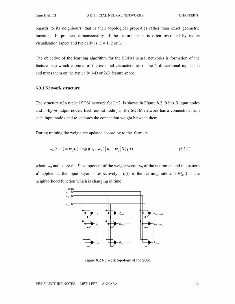
The structure of a typical SOM network for L=2 is shown in Figure 8.2. It has N input nodes
and m-by-m output nodes. Each output node j in the SOFM network has a connection from
each input node i and wij denotes the connection weight between them.
During training the weigts are updated acoording to the formula
),()w-)(uη()()1( iji tjNwuttwtw ijiijij −+=+ (8.3.1)
where wij and ui are the ith component of the weight vector wj of the neuron nj, and the pattern
uk applied at the input layer is respectively, η(t) is the learning rate and N(j,t) is the
neighborhood function which is changing in time
x n
x 1x 2
dm
d1
d2
d
d
d
2m
m+1
m+2
d
d
d
mxm
(m-1)m+1
(m-1)m+2
Inputs
Figure 8.2 Network topology of the SOM
Ugur HALICI ARTIFICIAL NEURAL NETWORKS CHAPTER 8
EE543 LECTURE NOTES . METU EEE . ANKARA
132
The learning algorithm captures two essential aspects of the map formation, namely,
competition and cooperation between neurons of the output lattice.
6.3.2 Competition
Competition determines the winning neuron dwin, whose weight vector is the one closest to the
applied input vector. For this purpose the input vector u is compared with each weight vector
wj from the weight matrix W and the index of the winning neuron nwin is established
considering the following formula.
j
jwinn wu −= minarg (8.3.2)
6.3.3 Cooperation
All neurons nj located in a topological neighbourhood of the winning neurons nwin will have
their weights updated usually with a strength Ν(j) related to their distance d(j) from the
winning neuron, where d(j) can be calculated using the formula
)pos()pos()( winj nnjd −= (8.3.3)
where pos(.) is the position of the neuron in the lattice. As the norm city-block distance or
Euclidian distance can be used.
6.3.4 Neighbourhood Function
In its simplest form, a neighbourhood is rectengular
⎩⎨⎧
>≤
=)D()(0)D()(1
),(tjdtjd
tjN (8.3.4)
Ugur HALICI ARTIFICIAL NEURAL NETWORKS CHAPTER 8
EE543 LECTURE NOTES . METU EEE . ANKARA
133
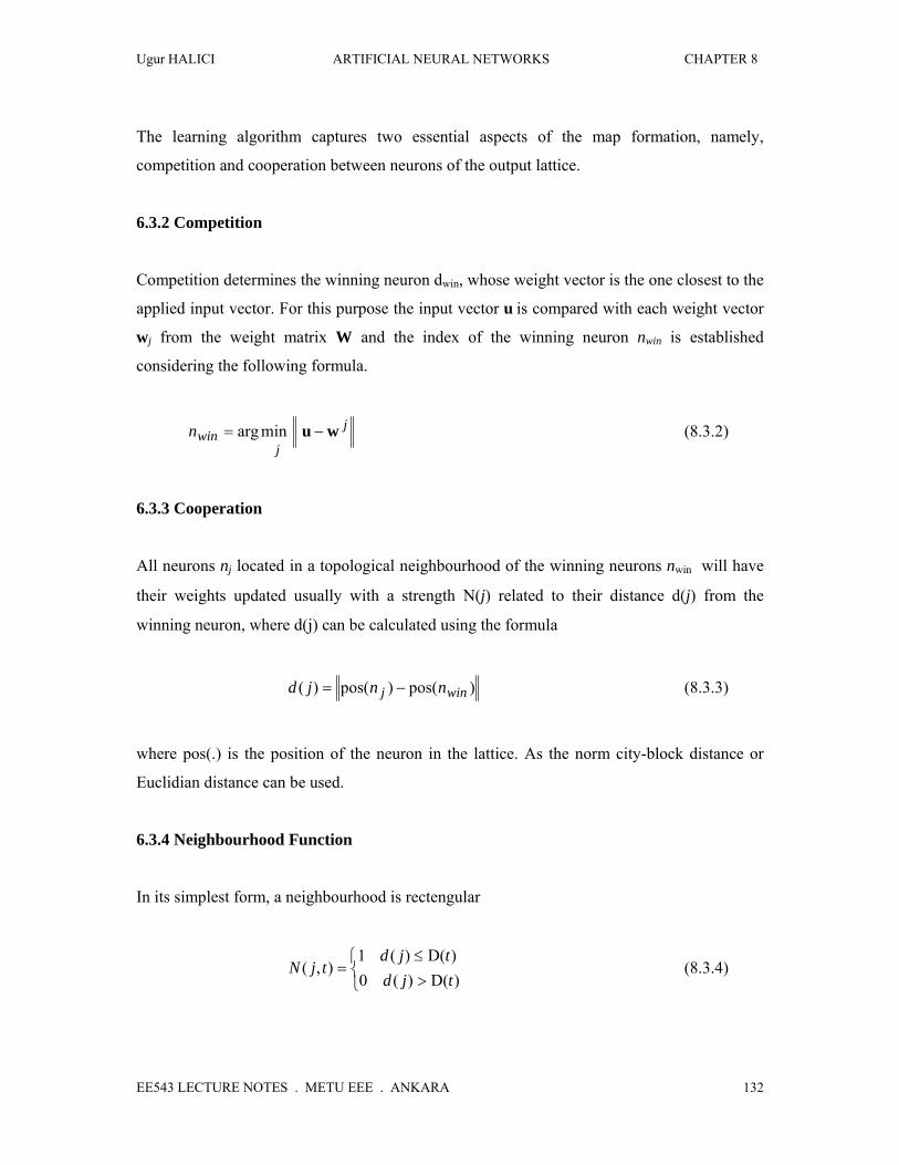
where N(j,t) is used instead of N(j) since D(t) is a threshold value decreased via a cooling
schedule as training progresses. For this neighbourhood function the distance is determined
considering the distance in the lattice in each dimension, and the one having the maximum
value is chosen as d(j). For L=2, N(j) corresponds to a square around nwin having side
length=2D(t)+1. The weights of all neurons within this square are updated with N(j)=1, while
the others remaining unchanged. As the training progresses, this neighbourhood gets smaller
and smaller, resulting in that only the neurons very close to the winner are updated towards
the end of the training. The training end as remains no more neuron in the neighbourhood.
(See Figure 8.3)
Figure 8.3. Threshold neighbourhood, narrowing as training progresses
Usually, the neighbourhood function, Ν(j), is chosen as an L-dimensional Gausssian function:
))σ(2)d(exp(),N( 2
2
tjtj −
= (8.3.5)
where σ2 is the variance parameter specifying the spread of the Gaussian function and it is
decreasing as the training progresses as training progresses. Again σ is decresed Example of a
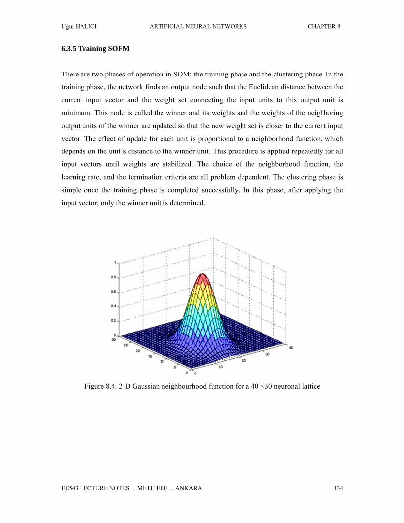
2-D Gaussian neighbourhood function is given in Figure 8.4.
Ugur HALICI ARTIFICIAL NEURAL NETWORKS CHAPTER 8
EE543 LECTURE NOTES . METU EEE . ANKARA
134
6.3.5 Training SOFM
There are two phases of operation in SOM: the training phase and the clustering phase. In the
training phase, the network finds an output node such that the Euclidean distance between the
current input vector and the weight set connecting the input units to this output unit is
minimum. This node is called the winner and its weights and the weights of the neighboring
output units of the winner are updated so that the new weight set is closer to the current input
vector. The effect of update for each unit is proportional to a neighborhood function, which
depends on the unit’s distance to the winner unit. This procedure is applied repeatedly for all
input vectors until weights are stabilized. The choice of the neighborhood function, the
learning rate, and the termination criteria are all problem dependent. The clustering phase is
simple once the training phase is completed successfully. In this phase, after applying the
input vector, only the winner unit is determined.
Figure 8.4. 2-D Gaussian neighbourhood function for a 40 ×30 neuronal lattice
Ugur HALICI ARTIFICIAL NEURAL NETWORKS CHAPTER 8
EE543 LECTURE NOTES . METU EEE . ANKARA
135
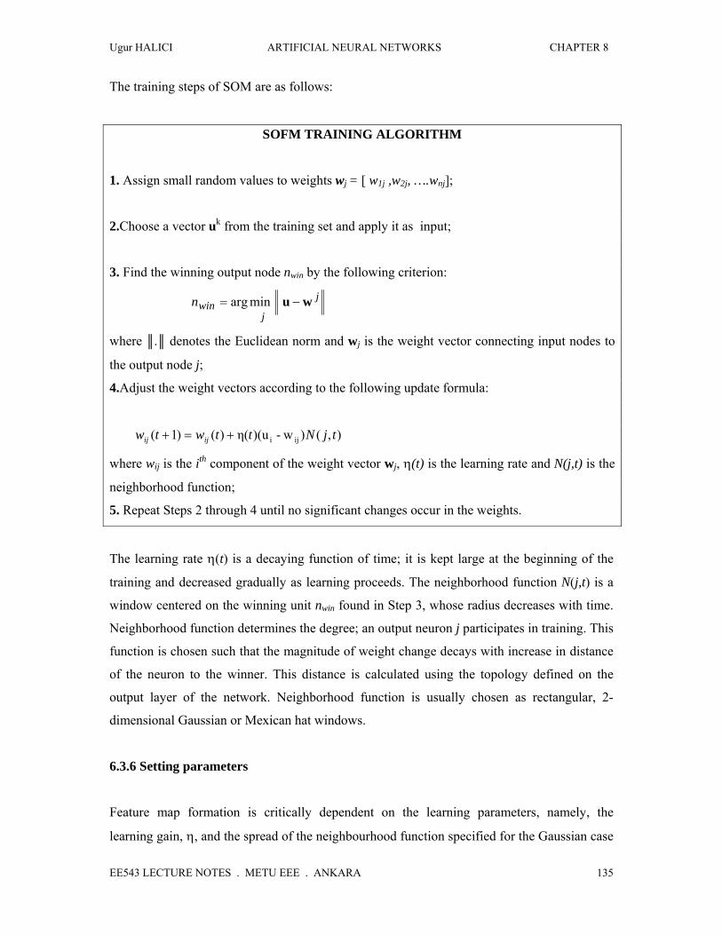
The training steps of SOM are as follows:
SOFM TRAINING ALGORITHM
1. Assign small random values to weights wj = [ w1j ,w2j, ….wnj];
2.Choose a vector uk from the training set and apply it as input;
3. Find the winning output node nwin by the following criterion:
j
jwinn wu −= minarg
where ║.║ denotes the Euclidean norm and wj is the weight vector connecting input nodes to
the output node j;
4.Adjust the weight vectors according to the following update formula:
),()w-)(uη()()1( iji tjNttwtw ijij +=+
where wij is the ith component of the weight vector wj, η(t) is the learning rate and N(j,t) is the
neighborhood function;
5. Repeat Steps 2 through 4 until no significant changes occur in the weights.
The learning rate η(t) is a decaying function of time; it is kept large at the beginning of the
training and decreased gradually as learning proceeds. The neighborhood function N(j,t) is a
window centered on the winning unit nwin found in Step 3, whose radius decreases with time.
Neighborhood function determines the degree; an output neuron j participates in training. This
function is chosen such that the magnitude of weight change decays with increase in distance
of the neuron to the winner. This distance is calculated using the topology defined on the
output layer of the network. Neighborhood function is usually chosen as rectangular, 2-
dimensional Gaussian or Mexican hat windows.
6.3.6 Setting parameters
Feature map formation is critically dependent on the learning parameters, namely, the
learning gain, η, and the spread of the neighbourhood function specified for the Gaussian case
Ugur HALICI ARTIFICIAL NEURAL NETWORKS CHAPTER 8
EE543 LECTURE NOTES . METU EEE . ANKARA
136
by the variance, σ2. In general, both parameters should be time-varying, but their values are
selected experimentally.
Usually, the learning gain should stay close to unity during the ordering phase of the
algorithm which can last for, say, 1000 iteration. After that, during the convergence phase,
should be reduced to reach the value of, say, 0.1.
The spread of the neighbourhood function should initially include all neurons for any winning
neuron and during the ordering phase should be slowly reduced to eventually include only a
few neurons in the winner's neighbourhood. During the convergence phase, the
neighbourhood function should include only the winning neuron.
6.3.7 Topological mapping
In SOFM the neurons are located on a discrete lattice. In training not only the winning neuron
but also its neighbors on the lattice are allowed to learn. This is the reason why neighboring
neurons gradually specialize to represent similar inputs, and the representations become
ordered on the map lattice. As the training progresses, the winning unit and its neighbors
adapt to represent the input even better by modifying their reference vectors towards the
current input. This topological map also reflect the underlying distribution of the input vectors
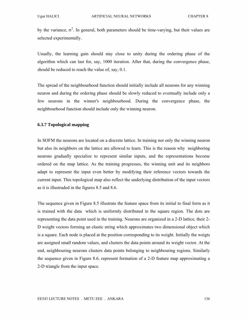
as it is illustraded in the figures 8.5 and 8.6.
The sequence given in Figure 8.5 illustrate the feature space from its initial to final form as it
is trained with the data which is uniformly distributed in the square region. The dots are
representing the data point used in the training. Neurons are organized in a 2-D lattice, their 2-
D weight vectors forming an elastic string which approximates two dimensional object which
is a square. Each node is placed at the position corresponding to its weight. Initially the weigts
are assigned small random values, and clusters the data points around its weight vector. At the
end, neighbouring neurons clusters data points belonging to neighbouring regions. Similarly
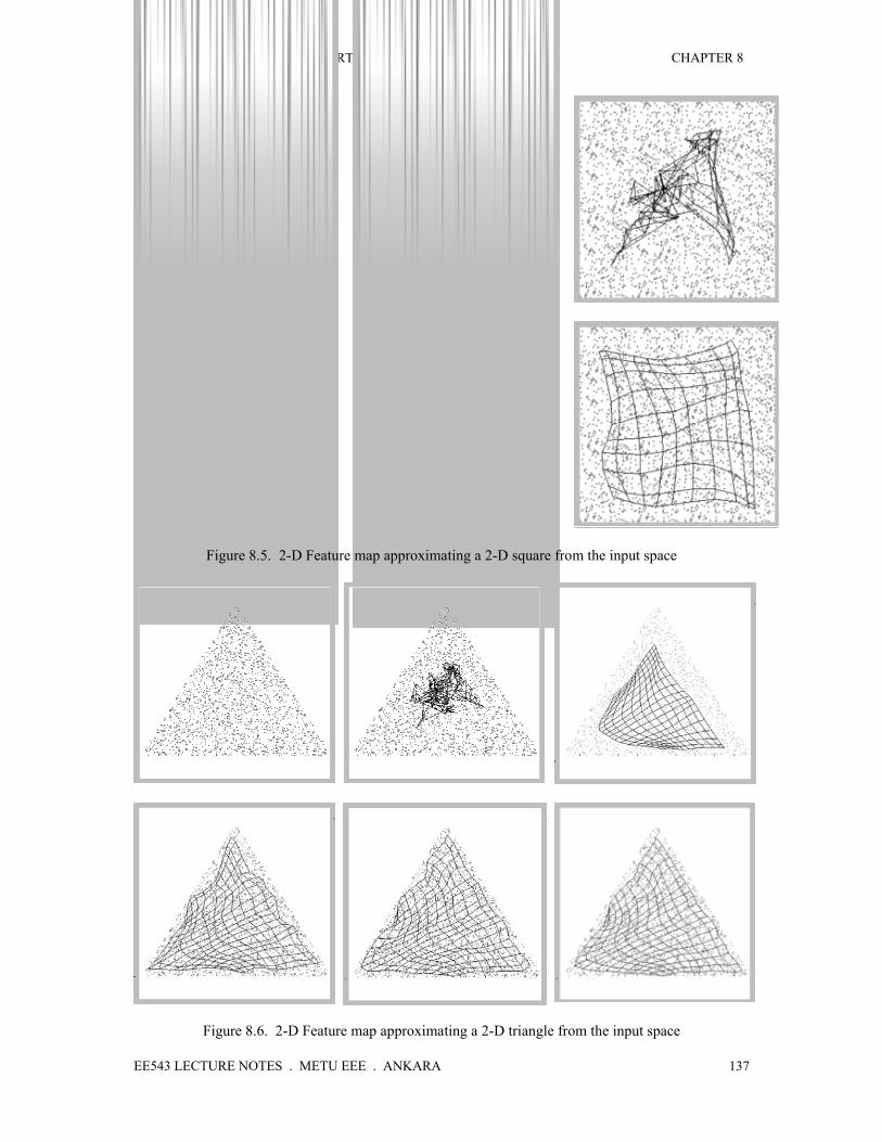
the sequence given in Figure 8.6, represent formation of a 2-D feature map approximating a
2-D triangle from the input space.
Ugur HALICI ARTIFICIAL NEURAL NETWORKS CHAPTER 8
EE543 LECTURE NOTES . METU EEE . ANKARA
137
Figure 8.5. 2-D Feature map approximating a 2-D square from the input space
Figure 8.6. 2-D Feature map approximating a 2-D triangle from the input space
Ugur HALICI ARTIFICIAL NEURAL NETWORKS CHAPTER 8
EE543 LECTURE NOTES . METU EEE . ANKARA
138
6. 4. SOFM versus K-means clustrering
Rigorous mathematical treatment of the SOM algorithm has turned out to be extremely
difficult in general (Kangas, 1994; and Kohonen, 1995). In the case of a discrete data set and
a fixed neighborhood kernel, however, there exists an error function for the SOM, namely
[Kohonen, 1991, Ritter and Schulten, 1988]
∑ ∑∈
−=k Cn
ki
cki
kE
2α mu (8.4.1)
The weight update rule of the SOM, corresponds to a gradient descent step in minimizing the
above error function
6.4.1 Relation to K-means clustering.
The cost function of the SOM, Equation (8.4.1), closely resembles Equation (8.2.1), which the
K-means clustering algorithm tries to minimize. The difference is that in the SOM the
distance of each input from all of the reference vectors instead of just the closest one is taken
into account, weighted by the neighborhood kernel h. Thus, the SOM functions as a
conventional clustering algorithm if the width of the neighborhood kernel is zero.
The close relation between the SOM and the K-means clustering algorithm also hints at why
the self-organized map follows rather closely the distribution of the data set in the input
space: it is known for vector quantization that the density of the reference vectors
approximates the density of the input vectors for high-dimensional data [Kohonen, 1995c,
Zador, 1982], and K-means is essentially equivalent to vector quantization. In fact, an
expression for the density of the reference vectors of the SOM has been derived in the one-
dimensional case [Ritter, 1991]; in the limit of a very wide neighborhood and a large number
of reference vectors the density is proportional to p(u)2/3, where p(u) is the probability
density function of the input data.