2-1 Copyright © 2013 Pearson Education, Inc. publishing as Prentice Hall

Chapter Two: Linear Programming: Model Formulation and Graphical Solution PROBLEM SUMMARY

1. Maximization (1–28 continuation), graphical solution

2. Maximization, graphical solution

3. Minimization, graphical solution

4. Sensitivity analysis (2–3)

5. Minimization, graphical solution

6. Maximization, graphical solution

7. Slack analysis (2–6)

8. Sensitivity analysis (2–6)

9. Maximization, graphical solution

10. Slack analysis (2–9)

11. Maximization, graphical solution

12. Minimization, graphical solution

13. Maximization, graphical solution

14. Sensitivity analysis (2–13)

15. Sensitivity analysis (2–13)

16. Maximization, graphical solution

17. Sensitivity analysis (2–16)

18. Maximization, graphical solution

19. Sensitivity analysis (2–18)

20. Maximization, graphical solution

21. Standard form (2–20)

22. Maximization, graphical solution

23. Standard form (2–22)

24. Maximization, graphical solution

25. Constraint analysis (2–24)

26. Minimization, graphical solution

27. Sensitivity analysis (2–26)

28. Sensitivity analysis (2–26)

29. Sensitivity analysis (2–22)

30. Minimization, graphical solution

31. Minimization, graphical solution

32. Sensitivity analysis (2–31)

33. Minimization, graphical solution

34. Maximization, graphical solution

35. Minimization, graphical solution

36. Maximization, graphical solution

37. Sensitivity analysis (2–34)

38. Minimization, graphical solution

39. Maximization, graphical solution

40. Maximization, graphical solution

41. Sensitivity analysis (2–38)

42. Maximization, graphical solution

43. Sensitivity analysis (2–40)

44. Maximization, graphical solution

45. Sensitivity analysis (2–42)

46. Minimization, graphical solution

47. Sensitivity analysis (2–44)

48. Maximization, graphical solution

49. Sensitivity analysis (2–46)

50. Maximization, graphical solution

51. Sensitivity analysis (2–48)

52. Maximization, graphical solution

53. Minimization, graphical solution

54. Sensitivity analysis (2–53)

55. Minimization, graphical solution

56. Sensitivity analysis (2–55)

57. Maximization, graphical solution

58. Minimization, graphical solution

59. Sensitivity analysis (2–52)

60. Maximization, graphical solution

61. Sensitivity analysis (2–54)

62. Multiple optimal solutions

63. Infeasible problem

64. Unbounded problem

PROBLEM SOLUTIONS

1. a) x1 = # cakes x2 = # loaves of bread maximize Z = $10x1 + 6x2

subject to 3x1 + 8x2 ≤ 20 cups of flour

45x1 + 30x2 ≤ 180 minutes x1,x2 ≥ 0

2-2 Copyright © 2013 Pearson Education, Inc. publishing as Prentice Hall

b)

0 2 4 6 8 10 12 14x

x

1

optimal

B

C

A2

4

6

8

10

12

2

A: x1 = 0x2 = 2.5Z = 15

B: x1 = 3.1x2 = 1.33Z = 38.98

*C: x1 = 4x2 = 0Z = 40

2. a) Maximize Z = 6x1 + 4x2 (profit, $) subject to

10x1 + 10x2 ≤ 100 (line 1, hr) 7x1 + 3x2 ≤ 42 (line 2, hr)

x1,x2 ≥ 0

b)

12

14

10

8

6

4

2

A : x1 = 0

A

C

B

x1

x2

Z

0 2 4 6 8 10 12 14

BPoint is optimal

x2 = 10

Z = 40

*B : x1 = 3

x2 = 7

Z = 46

C : x1 = 6

x2 = 0

Z = 36

3. a) Minimize Z = .05x1 + .03x2 (cost, $) subject to

8x1 + 6x2 ≥ 48 (vitamin A, mg) x1 + 2x2 ≥ 12 (vitamin B, mg)

x1,x2 ≥ 0

b)

12

10

8

6

4

2

B

C

A

x1

x2

Z

0 2 4 6 8 10 12 14

Point A is optimal

*A : x1 = 0

x2 = 8

Z = .24

B : x1 = 12/5

x2 = 24/5

Z = .26

C : x1 = 12

x2 = 0

Z = .60

4. The optimal solution point would change from point A to point B, thus resulting in the optimal solution

x1 = 12/5 x2 = 24/5 Z = .408

5. a) Minimize Z = 3x1 + 5x2 (cost, $) subject to

10x1 + 2x2 ≥ 20 (nitrogen, oz) 6x1 + 6x2 ≥ 36 (phosphate, oz)

x2 ≥ 2 (potassium, oz) x1,x2 ≥ 0

b)

12

10

8

6

4

2

A

B

C

x1

x2

Z0 2 4 6 8 10 12 14

Point C is optimal

A : x1 = 0

x2 = 10

Z = 50

B : x1 = 1

x2 = 5

Z = 28

*C : x1 = 4

x2 = 2

Z = 22

6. a) Maximize Z = 400x1 + 100x2 (profit, $)

subject to

8x1 + 10x2 ≤ 80 (labor, hr) 2x1 + 6x2 ≤ 36 (wood)

x1 ≤ 6 (demand, chairs) x1,x2 ≥ 0

2-3 Copyright © 2013 Pearson Education, Inc. publishing as Prentice Hall

b)

12

10

8

6

4

2

A

B

C

D x1

x2

Z

0 2 4 6 8 10 12 14 16 18

Point C is optimal

A : x1 = 0

x2 = 6

Z = 600

B : x1 = 30/7

x2 = 32/7

Z = 2,171

D : x1 = 6

x2 = 0

Z = 2,400

C : x1 = 6

x2 = 3.2

Z = 2,720

*

7. In order to solve this problem, you must substitute the optimal solution into the resource constraint for wood and the resource constraint for labor and determine how much of each resource is left over.

Labor

8x1 + 10x2 ≤ 80 hr 8(6) + 10(3.2) ≤ 80

48 + 32 ≤ 80 80 ≤ 80

There is no labor left unused.

Wood

2x1 + 6x2 ≤ 36 2(6) + 6(3.2) ≤ 36

12 + 19.2 ≤ 36 31.2 ≤ 36

36 − 31.2 = 4.8

There is 4.8 lb of wood left unused.

8. The new objective function, Z = 400x1 + 500x2, is parallel to the constraint for labor, which results in multiple optimal solutions. Points B (x1 = 30/7, x2 = 32/7) and C (x1 = 6, x2 = 3.2) are the alternate optimal solutions, each with a profit of $4,000.

9. a) Maximize Z = x1 + 5x2 (profit, $) subject to

5x1 + 5x2 ≤ 25 (flour, lb) 2x1 + 4x2 ≤ 16 (sugar, lb)

x1 ≤ 5 (demand for cakes) x1,x2 ≥ 0

b)

12

10

8

6

4

2

B

C

A

x1

x2

Z

0 2 4 6 8 10 12 14

Point A is optimal

A : x1 = 0

x2 = 4

Z = 20

B : x1 = 2

x2 = 3

Z = 17

C : x1 = 5

x2 = 0

Z = 5

*

10. In order to solve this problem, you must substitute the optimal solution into the resource constraints for flour and sugar and determine how much of each resource is left over.

Flour

5x1 + 5x2 ≤ 25 lb 5(0) + 5(4) ≤ 25

20 ≤ 25 25 − 20 = 5

There are 5 lb of flour left unused.

Sugar

2x1 + 4x2 ≤ 16 2(0) + 4(4) ≤ 16

16 ≤ 16

There is no sugar left unused.

11.

12

10

8

6

4

2

A

B

CZ

x1

x2

0 2 4 6 8 10 12

Point A is optimal

A : x1 = 0

x2 = 9

Z = 54

B : x1 = 4

x2 = 3

Z = 30

C : x1 = 4

x2 = 1

Z = 18

*

12. a) Minimize Z = 80x1 + 50x2 (cost, $) subject to

3x1 + x2 ≥ 6 (antibiotic 1, units) x1 + x2 ≥ 4 (antibiotic 2, units)

2-4 Copyright © 2013 Pearson Education, Inc. publishing as Prentice Hall

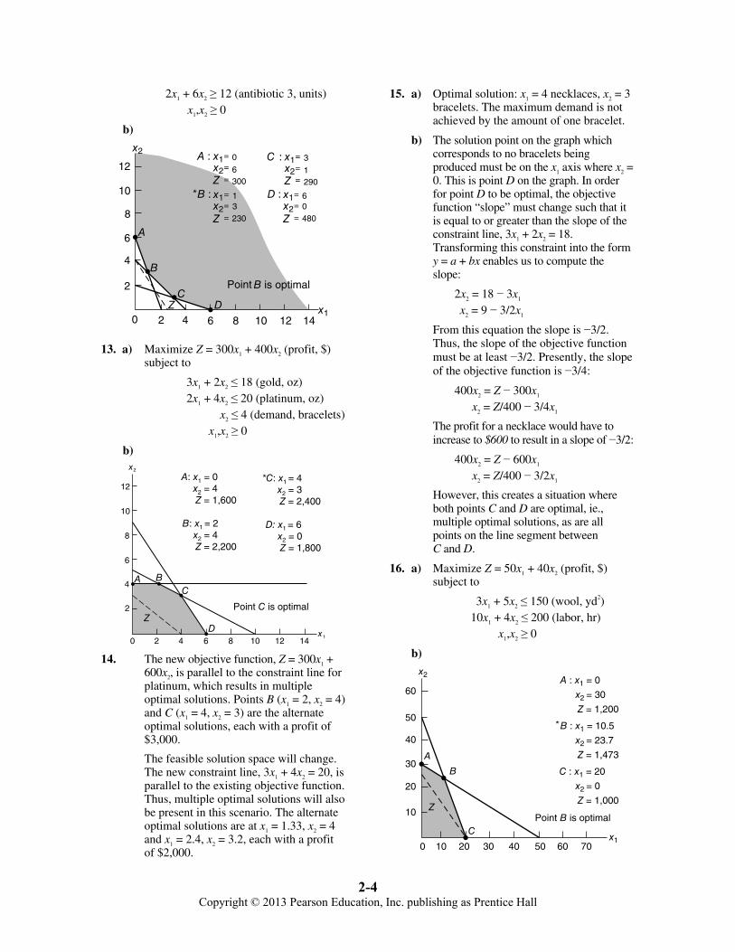
2x1 + 6x2 ≥ 12 (antibiotic 3, units) x1,x2 ≥ 0

b)

12

10

8

6

4

2

B

B

A :

A

C

C D

x1

x1

x2

x2

B :

Z

ZZ

Z

===

x1x2

===

x1x2

===0

6300

230

3

1290

13

D :

Z

x1x2

===

480

60

0 2 4 6 8 10 12 14

Point is optimal

*

:

13. a) Maximize Z = 300x1 + 400x2 (profit, $) subject to

3x1 + 2x2 ≤ 18 (gold, oz) 2x1 + 4x2 ≤ 20 (platinum, oz)

x2 ≤ 4 (demand, bracelets) x1,x2 ≥ 0

b)

0 2 4 6 8 10 12 14x

x

1

Point C is optimalZ

C

D

BA

2

4

6

8

10

12

2

A: x1 = 0x2 = 4Z = 1,600

B: x1 = 2x2 = 4Z = 2,200

*C: x1 = 4x2 = 3Z = 2,400

D: x1 = 6x2 = 0Z = 1,800

14. The new objective function, Z = 300x1 + 600x2, is parallel to the constraint line for platinum, which results in multiple optimal solutions. Points B (x1 = 2, x2 = 4) and C (x1 = 4, x2 = 3) are the alternate optimal solutions, each with a profit of $3,000.

The feasible solution space will change. The new constraint line, 3x1 + 4x2 = 20, is parallel to the existing objective function. Thus, multiple optimal solutions will also be present in this scenario. The alternate optimal solutions are at x1 = 1.33, x2 = 4 and x1 = 2.4, x2 = 3.2, each with a profit of $2,000.

15. a) Optimal solution: x1 = 4 necklaces, x2 = 3 bracelets. The maximum demand is not achieved by the amount of one bracelet.

b) The solution point on the graph which corresponds to no bracelets being produced must be on the x1 axis where x2 = 0. This is point D on the graph. In order for point D to be optimal, the objective function “slope” must change such that it is equal to or greater than the slope of the constraint line, 3x1 + 2x2 = 18. Transforming this constraint into the form y = a + bx enables us to compute the slope:

2x2 = 18 − 3x1 x2 = 9 − 3/2x1

From this equation the slope is −3/2. Thus, the slope of the objective function must be at least −3/2. Presently, the slope of the objective function is −3/4:

400x2 = Z − 300x1 x2 = Z/400 − 3/4x1

The profit for a necklace would have to increase to $600 to result in a slope of −3/2:

400x2 = Z − 600x1 x2 = Z/400 − 3/2x1

However, this creates a situation where both points C and D are optimal, ie., multiple optimal solutions, as are all points on the line segment between C and D.

16. a) Maximize Z = 50x1 + 40x2 (profit, $) subject to

3x1 + 5x2 ≤ 150 (wool, yd2) 10x1 + 4x2 ≤ 200 (labor, hr)

x1,x2 ≥ 0

b)

60

40

50

30

20

10

A

C

B

x1

x2

Z

0 10 20 30 40 50 60 70

Point B is optimal

A : x1 = 0

x2 = 30

Z = 1,200

B : x1 = 10.5

x2 = 23.7

Z = 1,473

C : x1 = 20

x2 = 0

Z = 1,000

*

2-5 Copyright © 2013 Pearson Education, Inc. publishing as Prentice Hall

17. The feasible solution space changes from the area 0ABC to 0AB'C', as shown on the following graph.

60

40

50

30

20

10

A

C C ′

B B ′

x1

x2

Z

0 10 20 30 40 50 60 70 The extreme points to evaluate are now A, B', and C'.

A: x1 = 0 x2 = 30 Z = 1,200

*B': x1 = 15.8 x2 = 20.5 Z = 1,610

C': x1 = 24 x2 = 0 Z = 1,200

Point B' is optimal

18. a) Maximize Z = 23x1 + 73x2 subject to

x1 ≤ 40 x2 ≤ 25

x1 + 4x2 ≤ 120 x1,x2 ≥ 0

b)

100

90

80

70

60

50

40

30

20

10

10 20 30 40 50 60 70 80 90 100 110 1200

C optimal,x1 = 40x2 = 20Z = 2,380

x2

x1

AB

C

D

19. a) No, not this winter, but they might after they recover equipment costs, which should be after the 2nd winter.

b) x1 = 55 x2 = 16.25 Z = 1,851

No, profit will go down

c) x1 = 40 x2 = 25

Z = 2,435

Profit will increase slightly

d) x1 = 55 x2 = 27.72 Z = $2,073

Profit will go down from (c)

20.

12

10

8

6

4

2

A

BC x1

x2

Z

0 2 4 6 8 10 12 14

Point B is optimal

A : x1 = 0

x2 = 5

Z = 5

B : x1 = 4

x2 = 1

Z = 7

C : x1 = 4

x2 = 0

Z = 6

*

21. Maximize Z = 1.5x1 + x2 + 0s1 + 0s2 + 0s3

subject to

x1 + s1 = 4 x2 + s2 = 6

x1 + x2 + s3 = 5 x1,x2 ≥ 0

A: s1 = 4, s2 = 1, s3 = 0 B: s1 = 0, s2 = 5, s3 = 0 C: s1 = 0, s2 = 6, s3 = 1

22.

12

10

8

6

4

2

A

B

Cx1

x2

Z

0 2 4 6 8 10 12 14 16 2018

Point B is optimal

A : x1 = 0

x2 = 10

Z = 80

B : x1 = 8

x2 = 5.2

Z = 81.6

C : x1 = 8

x2 = 0

Z = 40

*

2-6 Copyright © 2013 Pearson Education, Inc. publishing as Prentice Hall

23. Maximize Z = 5x1 + 8x2 + 0s1 + 0s3 + 0s4

subject to 3x1 + 5x2 + s1 = 50 2x1 + 4x2 + s2 = 40 x1 + s3 = 8 x2 + s4 = 10

x1,x2 ≥ 0 A: s1 = 0, s2 = 0, s3 = 8, s4 = 0 B: s1 = 0, s2 = 3.2, s3 = 0, s4 = 4.8 C: s1 = 26, s2 = 24, s3 = 0, s4 = 10

24.

12

14

16

10

8

6

4

2

A B

Cx1

x2

Z

0 2 4 6 8 10 12 14 16 18 20

Point B is optimal

A : x1 = 8

x2 = 6

Z = 112

B : x1 = 10

x2 = 5

Z = 115

C : x1 = 15

x2 = 0

Z = 97.5

*

25. It changes the optimal solution to point A (x1 = 8, x2 = 6, Z = 112), and the constraint, x1 + x2 ≤ 15, is no longer part of the solution space boundary.

26. a) Minimize Z = 64x1 + 42x2 (labor cost, $) subject to

16x1 + 12x2 ≥ 450 (claims) x1 + x2 ≤ 40 (workstations)

0.5x1 + 1.4x2 ≤ 25 (defective claims) x1,x2 ≥ 0

b) x2

x1

BC

DA

0 5 10 15 20 25 30 35 40 45 50

5

10

15

20

25

30

35

40

45

50

Point B is optimal

A : x1 = 28.125

x2 = 0

Z = 1,800

B : x1 = 20.121

x2 = 10.670

Z = 1,735.97

C : x1 = 5.55

x2 = 34.45

Z = 2,437.9

* D : x1 = 40

x2 = 0

Z = 2,560

27. Changing the pay for a full-time claims processor from $64 to $54 will change the solution to point A in the graphical solution where x1 = 28.125 and x2 = 0, i.e., there will be no part-time operators. Changing the pay for a part-time operator from $42 to $36 has no effect on the number of full-time and part-time operators hired, although the total cost will be reduced to $1,671.95.

28. Eliminating the constraint for defective claims would result in a new solution, x1 = 0 and x2 = 37.5, where only part-time operators would be hired.

29. The solution becomes infeasible; there are not enough workstations to handle the increase in the volume of claims.

30.

x1

x2

0–2–4–6 2 4 6 8 10 12

12

10

8

6

4

2

Point B is optimal

A : x1 = 2

x2 = 6

Z = 52

B : x1 = 4

x2 = 2

Z = 44

C : x1 = 6

x2 = 0

Z = 48

*

A

B

C

Z

31.

12

10

8

6

4

2BA

D

Cx1

x2

(5)

(2)

(3)

(4)

(1)

0 2 4 6 8 10 12

Point C is optimal

A : x1 = 2.67x2 = 2.33

Z = 22

B : x1 = 4x2 = 3

Z = 30

D : x1 = 3.36x2 = 3.96

Z = 33.84

C : x1 = 4x2 = 1

Z = 18

*

32. The problem becomes infeasible.

2-7 Copyright © 2013 Pearson Education, Inc. publishing as Prentice Hall

33.

12

10

8

6

4

2B

A

x1

x2

0 2 4 6 8 10 12 14

Feasible space

Point A is optimal

*A : x1 = 4.8

x2 = 2.4

Z = 26.4

B : x1 = 6

x2 = 1.5

Z = 31.5

34.

A

C

B

x1

x2

0–2

–2

–4

–4

–6

–6

–8

–8

–10 2 4 6 8 10 12

12

10

8

6

4

2

Point B is optimal

A : x1 = 4x2 = 3.5

Z = 19

B : x1 = 5x2 = 3

Z = 21

C : x1 = 4x2 = 1

Z = 14

*

35.

12

10

8

6

4

2

–2

B

A

x1

x2

02 6 8 10 12 14

C

Point A is optimal

A : x1 = 3.2

x2 = 6

Z = 37.6

B : x1 = 5.33

x2 = 3.33

Z = 49.3

C : x1 = 9.6

x2 = 1.2

Z = 79.2

*

4

36. a) Maximize Z = $4.15x1 + 3.60x2 (profit, $) subject to

1 2

1 2

11 2

2

1 2

115 (freezer space, gals.)

0.93 0.75 90 (budget, $)

2or 2 0 (demand)

1

, 0

x x

x x

xx x

x

x x

+ ≤+ ≤

≥ − ≥

≥

b)x2

x1

B

A

0 20 40 60 80 100 120

20

40

60

80

100

120

Point A is optimal

*A : x1 = 68.96

x2 = 34.48

Z = 410.35

B : x1 = 96.77

x2 = 0

Z = 401.6

37. No additional profit, freezer space is not a binding constraint.

38. a) Minimize Z = 200x1 + 160x2 (cost, $) subject to

6x1 + 2x2 ≥ 12 (high-grade ore, tons) 2x1 + 2x2 ≥ 8 (medium-grade ore, tons)

4x1 + 12x2 ≥ 24 (low-grade ore, tons) x1,x2 ≥ 0

b)

12

14

10

8

6

4

2

B

A

C D

x1

x2

0 2 4 6 8 10 12 14

Point B is optimal

A : x1 = 0

x2 = 6

Z = 960

B : x1 = 1

x2 = 3

Z = 680

C : x1 = 3

x2 = 1

Z = 760

D : x1 = 6

x2 = 0

Z = 1,200

*

2-8 Copyright © 2013 Pearson Education, Inc. publishing as Prentice Hall

39. a) Maximize Z = 800x1 + 900x2 (profit, $) subject to

2x1 + 4x2 ≤ 30 (stamping, days) 4x1 + 2x2 ≤ 30 (coating, days) x1 + x2 ≥ 9 (lots) x1,x2 ≥ 0

b)

12

14

10

8

6

4

2

BA

C

x1

x2

0 2 4 6 8 10 12 14 16

Point B is optimal

A : x1 = 3

x2 = 6

Z = 7,800

B : x1 = 5

x2 = 5

Z = 8,500

C : x1 = 6

x2 = 3

Z = 7,500

*

40. a) Maximize Z = 30x1 + 70x2 (profit, $) subject to

4x1 + 10x2 ≤ 80 (assembly, hr) 14x1 + 8x2 ≤ 112 (finishing, hr)

x1 + x2 ≤ 10 (inventory, units) x1,x2 ≥ 0

b)

12

14

10

8

6

4

2

A

BC

D x1

x2

0 2 4 6 8 10 12 14 16 2018

A : x1 = 0

x2 = 8

Z = 560

B : x1 = 3.3

x2 = 6.7

Z = 568

C : x1 = 5.3

x2 = 4.7

Z = 488

D : x1 = 8

x2 = 0

Z = 240

*

Point B is optimal

41. The slope of the original objective function is computed as follows:

Z = 30x1 + 70x2 70x2 = Z − 30x1 x2 = Z/70 − 3/7x1

slope = −3/7

The slope of the new objective function is computed as follows:

Z = 90x1 + 70x2 70x2 = Z − 90x1 x2 = Z/70 − 9/7x1

slope = −9/7

The change in the objective function not only changes the Z values but also results in a new solution point, C. The slope of the new objective function is steeper and thus changes the solution point.

A: x1 = 0 C: x1 = 5.3 x2 = 8 x2 = 4.7

Z = 560 Z = 806

B: x1 = 3.3 D: x1 = 8 x2 = 6.7 x2 = 0 Z = 766 Z = 720

42. a) Maximize Z = 9x1 + 12x2 (profit, $1,000s) subject to

4x1 + 8x2 ≤ 64 (grapes, tons) 5x1 + 5x2 ≤ 50 (storage space, yd3)

15x1 + 8x2 ≤ 120 (processing time, hr) x1 ≤ 7 (demand, Nectar) x2 ≤ 7 (demand, Red)

x1,x2 ≥ 0

b)

0 2 4 6 8 10 12 14 16 18

2

4

6

8

10

12

14

16

18

x2

x1

Optimal pointB

C

D

E

F

A

x2 = 7

Z = 84

x2 = 7

Z = 102

*C : x1 = 4

x2 = 6

Z = 108

D : x1 = 5.71

x2 = 4.28

Z = 102.79

E : x1 = 7

x2 = 1.875

Z = 85.5

F : x1 = 7

x2 = 0

Z = 63

A : x1 = 0

B : x1 = 2

43. a) 15(4) + 8(6) ≤ 120 hr 60 + 48 ≤ 120 108 ≤ 120 120 − 108 = 12 hr left unused

2-9 Copyright © 2013 Pearson Education, Inc. publishing as Prentice Hall

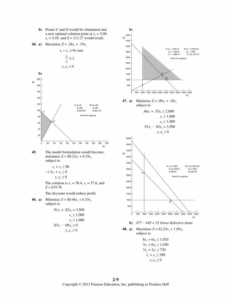
b) Points C and D would be eliminated and a new optimal solution point at x1 = 5.09, x2 = 5.45, and Z = 111.27 would result.

44. a) Maximize Z = .28x1 + .19x2

1 2

2

1

1 2

96 cans

2

, 0

x xxx

x x

+ ≤

≥

≥

b) 200

180

160

140

120

100

80

60

40

20

0 20 40 60 80 100 120 140 160 180 200

X1

X2

A

B

A: X1=0A: X2=96A: Z=$18.24

*B: X1=32*A: X2=64*A: Z=$21.12

Point B is optimal

45. The model formulation would become, maximize Z = $0.23x1 + 0.19x2 subject to

x1 + x2 ≤ 96 –1.5x1 + x2 ≥ 0

x1,x2 ≥ 0

The solution is x1 = 38.4, x2 = 57.6, and Z = $19.78

The discount would reduce profit.

46. a) Minimize Z = $0.46x1 + 0.35x2 subject to

.91x1 + .82x2 = 3,500 x1 ≥ 1,000 x2 ≥ 1,000

.03x1 − .06x2 ≥ 0 x1,x2 ≥ 0

b) 5000

4500

4000

3500

3000

2500

2000

1500

1000

500

X1

X2

A

B

A: X1 = 2,651.5A: X2 = 1,325.8A: Z = 1,683.71

B: X1 = 2,945.05*AX2 = 1,000*A Z = $1,704.72

Point A is optimal

0 500 2000 2500 3000 3500 4500 5000400015001000

47. a) Minimize Z = .09x1 + .18x2

subject to

.46x1 + .35x2 ≤ 2,000 x1 ≥ 1,000 x2 ≥ 1,000

.91x1 − .82x2 = 3,500 x1,x2 ≥ 0

5000

4500

4000

3500

3000

2500

2000

1500

1000

500

6000

5500

0 500 1000 1500 2000 2500 3000 3500 4000 4500 5000

X1

X2

A

B

A: X1=1,000A: X2=3,158.57A: Z=658.5

*B: X1=2,945.05*A: X2=1,000*A: Z=445.05

Point B is optimal

b) 477 − 445 = 32 fewer defective items

48. a) Maximize Z = $2.25x1 + 1.95x2 subject to

8x1 + 6x2 ≤ 1,920 3x1 + 6x2 ≤ 1,440 3x1 + 2x2 ≤ 720

x1 + x2 ≤ 288 x1,x2 ≥ 0

2-10 Copyright © 2013 Pearson Education, Inc. publishing as Prentice Hall

b) 500

450

400

350

300

250

200

150

100

50

0 50 100 150 200 250 300 350 400 450 500

X1

X2

A

B

A: X1=0A: X2=240A: Z=468

*B: X1=96*A: X2=192*A: Z=590.4

C: X1=240*A: X2=0*A: Z=540

Point B is optional

C

49. A new constraint is added to the model in

1

2

1.5xx

≥

The solution is x1 = 160, x2 = 106.67, Z = $568

500

450

400

350

300

250

200

150

100

50

0 50 100 150 200 250 300 350 400 450 500

X1

X2

A

B

*A: X1=160.07A: X2=106.67A: Z=568

B: X1=240*A: X2=0*A: Z=540

Point A is optimal

50. a) Maximize Z = 400x1 + 300x2 (profit, $) subject to

x1 + x2 ≤ 50 (available land, acres)

10x1 + 3x2 ≤ 300 (labor, hr)

8x1 + 20x2 ≤ 800 (fertilizer, tons)

x1 ≤ 26 (shipping space, acres)

x2 ≤ 37 (shipping space, acres)

x1,x2 ≥ 0

b)

120

100

80

60

40

20BA

DEF

C

x1

x2

0 20 40 60 80 100 120 140

A : x1 = 0

x2 = 37

Z = 11,100

B : x1 = 7.5

x2 = 37

Z = 14,100

D : x1 = 21.4

x2 = 28.6

Z = 17,143

E : x1 = 26

x2 = 13.3

Z = 14,390

C : x1 = 16.7

x2 = 33.3

Z = 16,680

F : x1 = 26

x2 = 0

Z = 10,400

*

Point D is optimal

51. The feasible solution space changes if the fertilizer constraint changes to 20x1 + 20x2 ≤ 800 tons. The new solution space is A'B'C'D'. Two of the constraints now have no effect.

120

100

80

60

40

20

x1

x2

0 20 40 60 80 100 120 140

C ′

B ′A′

D′ The new optimal solution is point C':

A': x1 = 0 *C': x1 = 25.71 x2 = 37 x2 = 14.29 Z = 11,100 Z = 14,571

B': x1 = 3 D': x1 = 26 x2 = 37 x2 = 0 Z = 12,300 Z = 10,400

52. a) Maximize Z = $7,600x1 + 22,500x2 subject to

x1 + x2 ≤ 3,500 x2/(x1 + x2) ≤ .40

.12x1 + .24x2 ≤ 600 x1,x2 ≥ 0

2-11 Copyright © 2013 Pearson Education, Inc. publishing as Prentice Hall

b)

0 500

500

1000 1500 2000 2500 3000 3500 4000 4500 5000

1000

1500

2000

2500

3000

3500

4000

4500

5000

A

B

Optimal solution - B

x1 = 2100x2 = 1400z = 47,460,000

x1

53. a) Minimize Z = $(.05)(8)x1 + (.10)(.75)x2

subject to

5x1 + x2 ≥ 800

1

2

5 1.5xx

=

8x1 + .75x2 ≤ 1,200 x1, x2 ≥ 0

x1 = 96 x2 = 320 Z = $62.40

b)

B optimal,x1 = 96x2 = 320 Z = 62.40

100

100

0

200

300

400

500

600

700

800

900

1000

1100

1200

1300

1400

1500

1600x2

x1200 300 400 500 600 700 800 900 1000

A

B

C

54. The new solution is

x1 = 106.67 x2 = 266.67 Z = $62.67

If twice as many guests prefer wine to beer, then the Robinsons would be approximately 10 bottles of wine short and they would have approximately 53 more bottles of beer than they need. The waste is more difficult to compute. The model in problem 53 assumes that the Robinsons are ordering more wine and beer than they need, i.e., a buffer, and thus there logically would be some waste, i.e., 5% of the wine and 10% of the beer. However, if twice as many guests prefer wine, then there would logically be no waste for wine but only for beer. This amount “logically” would be the waste from 266.67 bottles, or $20, and the amount from the additional 53 bottles, $3.98, for a total of $23.98.

55. a) Minimize Z = 3700x1 + 5100x2

subject to

x1 + x2 = 45

(32x1 + 14x2) / (x1 + x2) ≤ 21

.10x1 + .04x2 ≤ 6

1

1 2

.25( )x

x x≥

+

2

1 2.25

( )x

x x≥

+

x1, x2 ≥ 0

b)

50 10 15 20 25 30 35 40 45 50x1

x2

50

45

40

35

30

25

20

15

10

5

x1 = 17.5x2 = 27.5Z = $205,000

2-12 Copyright © 2013 Pearson Education, Inc. publishing as Prentice Hall

56. a) No, the solution would not change

b) No, the solution would not change

c) Yes, the solution would change to China (x1) = 22.5, Brazil (x2) = 22.5, and Z = $198,000.

57. a) x1 = $ invested in stocks x2 = $ invested in bonds maximize Z = $0.18x1 + 0.06x2 (average annual return) subject to

x1 + x2 ≤ $720,000 (available funds) x1/(x1 + x2) ≤ .65 (% of stocks) .22x1 + .05x2 ≤ 100,000 (total possible loss)

x1,x2 ≥ 0

b)

0 100

100

200

300

400

500

600

700

800

900

1000

200 300 400 500 600 700 800 900 1000(1000S)

(1000S)

A

B

C

x1

x2

B, optimal:x1 = 376,470.59

x2 = 343,526.41

z = 88,376.47

58. x1 = exams assigned to Brad x2 = exams assigned to Sarah minimize Z = .10x1 + .06x2

subject to x1 + x2 = 120

x1 ≤ (720/7.2) or 100 x2 ≤ 50(600/12)

x1,x2 ≥ 0

50

500

A

B

100

100

150

150 200 X1

X2

200

*A : x1 = 70

x2 = 50

Z = 10

B : x1 = 100

x2 = 20

Z = 11.2

optimal

59. If the constraint for Sarah’s time became x2 ≤ 55 with an additional hour then the solution point at A would move to x1 = 65, x2 = 55 and Z = 9.8. If the constraint for Brad’s time became x1 ≤ 108.33 with an additional hour then the solution point (A) would not change. All of Brad’s time is not being used anyway so assigning him more time would not have an effect.

One more hour of Sarah’s time would reduce the number of regraded exams from 10 to 9.8, whereas increasing Brad by one hour would have no effect on the solution. This is actually the marginal (or dual) value of one additional hour of labor, for Sarah, which is 0.20 fewer regraded exams, whereas the marginal value of Brad’s is zero.

60. a) x1 = # cups of Pomona x2 = # cups of Coastal Maximize Z = $2.05x1 + 1.85x2

subject to 16x1 + 16x2 ≤ 3,840 oz or (30 gal. × 128 oz) (.20)(.0625)x1 + (.60)(.0625)x2 ≤ 6 lbs.

Colombian (.35)(.0625)x1 + (.10)(.0625)x2 ≤ 6 lbs.

Kenyan (.45)(.0625)x1 + (.30)(.0625)x2 ≤ 6 lbs.

Indonesian x2/x1 = 3/2 x1,x2 ≥ 0

2-13 Copyright © 2013 Pearson Education, Inc. publishing as Prentice Hall

b) Solution: x1 = 87.3 cups x2 = 130.9 cups Z = $421.09

200

A

400

600

800

1000

2000 400 600 800 1000X1

X2

A : x1 = 87.3

x2 = 130.9

Z = 421.09

61. a) The only binding constraint is for Colombian; the constraints for Kenyan and Indonesian are nonbinding and there are already extra, or slack, pounds of these coffees available. Thus, only getting more Colombian would affect the solution.

One more pound of Colombian would increase sales from $421.09 to $463.20.

Increasing the brewing capacity to 40 gallons would have no effect since there is already unused brewing capacity with the optimal solution.

b) If the shop increased the demand ratio of Pomona to Coastal from 1.5 to 1 to 2 to 1 it would increase daily sales to $460.00, so the shop should spend extra on advertising to achieve this result.

62.

60

70

80

50

40

30

20

10

A

B

C

D x1

x2

0 10 20 30 40 50 60 70 80

Multiple optimal solutions; Aand B alternate optimal.

*A : x1 = 0

x2 = 60

Z = 60,000

*B : x1 = 10

x2 = 30

Z = 60,000

C : x1 = 33.33

x2 = 6.67

Z = 106,669

D : x1 = 60

x2 = 0

Z = 180,000

Multiple optimal solutions; A and B alternate optimal

63.

60

70

80

50

40

30

20

10

x1

x2

0 10 20 30 40 50 60 70 80

Infeasible Problem

64.

60

70

80

50

40

30

20

10

x1

x2

0 10–10 20–20 30 40 50 60 70 80

Unbounded Problem

2-14 Copyright © 2013 Pearson Education, Inc. publishing as Prentice Hall

CASE SOLUTION: METROPOLITAN POLICE PATROL

The linear programming model for this case problem is

Minimize Z = x/60 + y/45 subject to

2x + 2y ≥ 5 2x + 2y ≤ 12 y ≥ 1.5x x, y ≥ 0

The objective function coefficients are determined by dividing the distance traveled, i.e., x/3, by the travel speed, i.e., 20 mph. Thus, the x coefficient is x/3 ÷ 20, or x/60. In the first two constraints, 2x + 2y represents the formula for the perimeter of a rectangle.

The graphical solution is displayed as follows.

6

5

4

3

2

1

A

B

C

D

x

y

0 1 2 3 4 5 6 7

point Optimal

The optimal solution is x = 1, y = 1.5, and Z = 0.05. This means that a patrol sector is 1.5 miles by 1 mile and the response time is 0.05 hr, or 3 min.

CASE SOLUTION: “THE POSSIBILITY” RESTAURANT

The linear programming model formulation is

Maximize = Z = $12x1 + 16x2

subject to

x1 + x2 ≤ 60 .25x1 + .50x2 ≤ 20

x1/x2 ≥ 3/2 or 2x1 − 3x2 ≥ 0 x2/(x1 + x2) ≥ .10 or .90x2 − .10x1 ≥ 0

x1x2 ≥ 0

The graphical solution is shown as follows.

60

70

80

100

50

40

30

20

10

A

B

Cx1

x2

x1 x2

0 10 20 30 40 50 60 70 80 100

Optimal point

–2 3 0

x1–x2.90 .10 0

x1 x2+ 20.25 .50

x1 x2+ 60

A : x1 = 34.3

x2 = 22.8

Z = $776.23

*B : x1 = 40

x2 = 20

Z = $800optimal

C : x1 = 6

x2 = 54

Z = $744

Changing the objective function to Z = $16x1 + 16x2 would result in multiple optimal solutions, the end points being B and C. The profit in each case would be $960.

Changing the constraint from .90x2 − .10x1 ≥ 0 to .80x2 −.20x1 ≥ 0 has no effect on the solution.

CASE SOLUTION: ANNABELLE INVESTS IN THE MARKET

x1 = no. of shares of index fund x2 = no. of shares of internet stock fund

Maximize Z = (.17)(175)x1 + (.28)(208)x2 = 29.75x1 + 58.24x2

subject to

1 2

1

2

2

1

1 2

175 208 $120,000

.33

2

, 0

+ =

≥

≤

>

x xxxxx

x x

x1 = 203 x2 = 406 Z = $29,691.37

2

1

Eliminating the constraint .33x

x≥

will have no effect on the solution.

1

2

Eliminating the constraint 2x

x≤

will change the solution to x1 = 149, x2 = 451.55, Z = $30,731.52.

2-15 Copyright © 2013 Pearson Education, Inc. publishing as Prentice Hall

Increasing the amount available to invest (i.e., $120,000 to $120,001) will increase profit from Z = $29,691.37 to Z = $29,691.62 or approximately $0.25. Increasing by another dollar will increase profit by another $0.25, and increasing the amount available by one more dollar will again increase profit by $0.25. This

indicates that for each extra dollar invested a return of $0.25 might be expected with this investment strategy. Thus, the marginal value of an extra dollar to invest is $0.25, which is also referred to as the “shadow” or “dual” price as described in Chapter 3.