Chapter Three: Probability (continued)

1/29

3.4 The Normal Curve

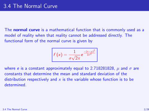
The normal curve is a mathematical function that is commonly used as amodel of reality when that reality cannot be addressed directly. Thefunctional form of the normal curve is given by

f (x) =1

σ√

2πe−(x−µ)2

2σ2

where e is a constant approximately equal to 2.718281828, µ and σ areconstants that determine the mean and standard deviation of thedistribution respectively and x is the variable whose function is to bedetermined.

3.4 The Normal Curve 2/29

Some Characteristics of the Normal Curve

1 The mean, median, and mode are all located at the center of thedistribution.

2 It is symmetric about its mean, median, and mode.

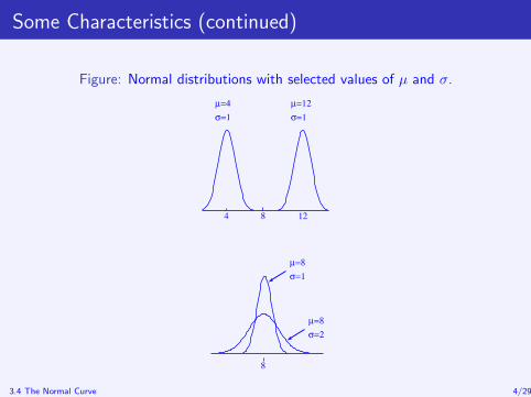
3 It is defined for all values of x between −∞ and ∞. This means thatdepictions such as those in the next slide show only a segment of thecurve since it stretches infinitely in either direction.

4 The area encompassed by the curve is equal to one regardless of thevalues of µ and σ.

3.4 The Normal Curve 3/29

Some Characteristics (continued)

Figure: Normal distributions with selected values of µ and σ.

4 8

8

12

µ=4

σ=1

µ=8

σ=1

µ=12

σ=1

µ=8

σ=2

3.4 The Normal Curve 4/29

Finding Areas Under The Normal Curve

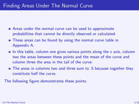
Areas under the normal curve can be used to approximateprobabilities that cannot be directly observed or calculated.

These areas can be found by using the normal curve table inAppendix A.

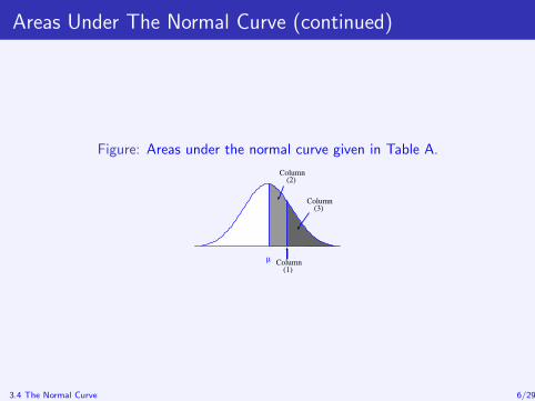
In this table, column one gives various points along the x axis, columntwo the areas between these points and the mean of the curve andcolumn three the area in the tail of the curve.

The areas in columns two and three sum to .5 because together theyconstitute half the curve.

The following figure demonstrates these points.

3.4 The Normal Curve 5/29

Areas Under The Normal Curve (continued)

Figure: Areas under the normal curve given in Table A.

µ

Column(2)

Column(3)

Column(1)

3.4 The Normal Curve 6/29

Areas Under The Normal Curve (continued)

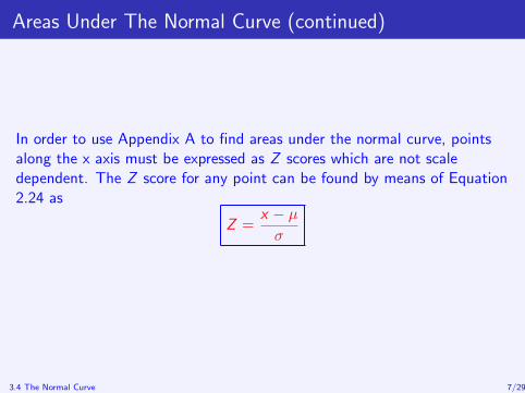
In order to use Appendix A to find areas under the normal curve, pointsalong the x axis must be expressed as Z scores which are not scaledependent. The Z score for any point can be found by means of Equation2.24 as

Z =x − µ

σ

3.4 The Normal Curve 7/29

Example

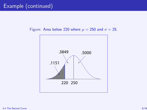
Given a normal curve with mean 250 and standard deviation 25, whatportion of the curve falls below 220?

3.4 The Normal Curve 8/29

Example (continued)

Figure: Area below 220 where µ = 250 and σ = 25.

.3849

.1151

.5000

250220

3.4 The Normal Curve 9/29

Solution

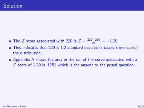
The Z score associated with 220 is Z = 220−25025 = −1.20.

This indicates that 220 is 1.2 standard deviations below the mean ofthe distribution.

Appendix A shows the area in the tail of the curve associated with aZ score of 1.20 is .1151 which is the answer to the posed question.

3.4 The Normal Curve 10/29

Example

Given a normal curve with mean 80 and standard deviation 10, find thearea between 65 and 85.

3.4 The Normal Curve 11/29

Example (continued)

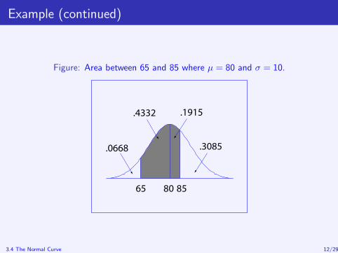
Figure: Area between 65 and 85 where µ = 80 and σ = 10.

.0668

.4332 .1915

.3085

65 80 85

3.4 The Normal Curve 12/29

Solution

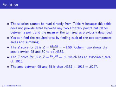
The solution cannot be read directly from Table A because this tabledoes not provide areas between any two arbitrary points but ratherbetween a point and the mean or the tail area as previously described.

You can find the required area by finding each of the two componentareas and summing.

The Z score for 65 is Z = 65−8010 = −1.50. Column two shows the

area between 65 and 80 to be .4332.

The Z score for 85 is Z = 85−8010 = .50 which has an associated area

of .1915.

The area between 65 and 85 is then .4332 + .1915 = .6247.

3.4 The Normal Curve 13/29

Example

Given a normal curve with mean 500 and standard deviation 50, find thearea between 555 and 600.

3.4 The Normal Curve 14/29

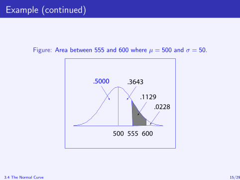
Example (continued)

Figure: Area between 555 and 600 where µ = 500 and σ = 50.

.5000

500 555 600

.3643

.0228

.1129

3.4 The Normal Curve 15/29

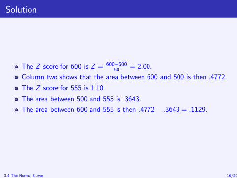
Solution

The Z score for 600 is Z = 600−50050 = 2.00.

Column two shows that the area between 600 and 500 is then .4772.

The Z score for 555 is 1.10

The area between 500 and 555 is .3643.

The area between 600 and 555 is then .4772− .3643 = .1129.

3.4 The Normal Curve 16/29

Example

Given a normal curve with mean .05 and standard deviation .01, find thearea below .0722.

3.4 The Normal Curve 17/29

Example (continued)

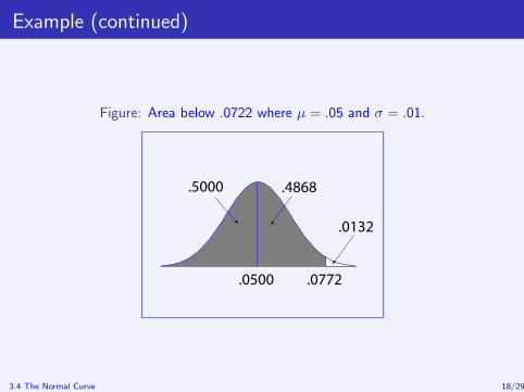
Figure: Area below .0722 where µ = .05 and σ = .01.

.0500 .0772

.5000 .4868

.0132

3.4 The Normal Curve 18/29

Solution

Because .05 is the mean of the distribution it has Z score 0.00 whichhas an associated tail area of .5.

The Z score for .0722 is Z = .0722−.0500.01 = 2.22.

Column two shows that the area between .0722 and .0500 is .4868.

The area below .0772 is then .5000 + .4868 = .9868.

3.4 The Normal Curve 19/29

Approximating Probabilities

When the relative frequency distribution of a population is not available,the normal curve may be used to approximate probabilities associated withthe population so long as the following two conditions are met.

1 The mean and standard deviation of the population are known.

2 The population relative frequency distribution is relatively normal inshape.

3.4 The Normal Curve 20/29

Example

Given a population of blood pressures with approximately normallydistributed relative frequency distribution and with mean and standarddeviation of 110.023 and 4.970 respectively, find the approximateprobability of randomly selecting a blood pressure from this population andfinding that it is 111.

3.4 The Normal Curve 21/29

Example (continued)

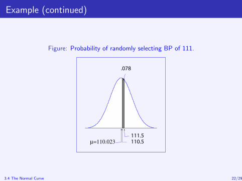
Figure: Probability of randomly selecting BP of 111.

111.5

110.5

.078

3.4 The Normal Curve 22/29

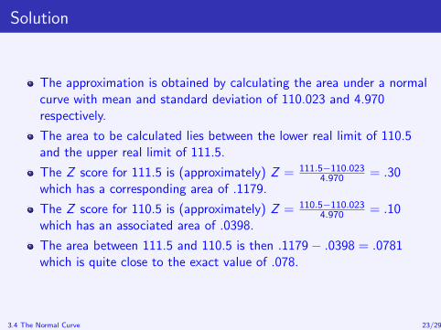
Solution

The approximation is obtained by calculating the area under a normalcurve with mean and standard deviation of 110.023 and 4.970respectively.

The area to be calculated lies between the lower real limit of 110.5and the upper real limit of 111.5.

The Z score for 111.5 is (approximately) Z = 111.5−110.0234.970 = .30

which has a corresponding area of .1179.

The Z score for 110.5 is (approximately) Z = 110.5−110.0234.970 = .10

which has an associated area of .0398.

The area between 111.5 and 110.5 is then .1179− .0398 = .0781which is quite close to the exact value of .078.

3.4 The Normal Curve 23/29

Example

Estimate the probability that the randomly selected observation is between100 and 105 (inclusive).

3.4 The Normal Curve 24/29

Example (continued)

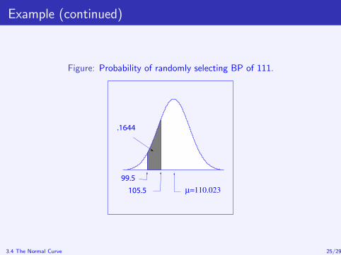
Figure: Probability of randomly selecting BP of 111.

105.5

99.5

.1644

3.4 The Normal Curve 25/29

Solution

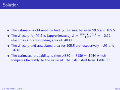
The estimate is obtained by finding the area between 99.5 and 105.5.

The Z score for 99.5 is (approximately) Z = 99.5−110.0234.970 = −2.12

which has a corresponding area of .4830.

The Z score and associated area for 105.5 are respectively −.91 and.3186.

The estimated probability is then .4830− .3186 = .1644 whichcompares favorably to the value of .161 calculated from Table 3.3.

3.4 The Normal Curve 26/29

Example

Estimate the probability that a randomly selected observation taken from apopulation with approximately normally distributed relative frequencydistribution and with mean and standard deviation of 110.023 and 4.970respectively will be greater than 103. Compare this estimate to the exactvalue computed from Table 3.3.

3.4 The Normal Curve 27/29

Example (continued)

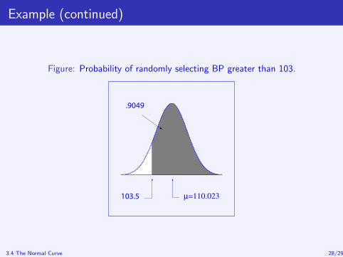
Figure: Probability of randomly selecting BP greater than 103.

103.5

.9049

3.4 The Normal Curve 28/29

Solution

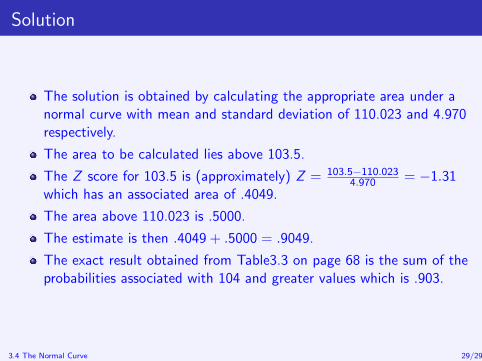
The solution is obtained by calculating the appropriate area under anormal curve with mean and standard deviation of 110.023 and 4.970respectively.

The area to be calculated lies above 103.5.

The Z score for 103.5 is (approximately) Z = 103.5−110.0234.970 = −1.31

which has an associated area of .4049.

The area above 110.023 is .5000.

The estimate is then .4049 + .5000 = .9049.

The exact result obtained from Table3.3 on page 68 is the sum of theprobabilities associated with 104 and greater values which is .903.

3.4 The Normal Curve 29/29