Chapter Three

Numerical Descriptive Measures

1.Age

4.Study / Week (hrs)

5. Auto Cost

($)

6.Alch bev /

wk (#)

7.Sodas / wk (#)

8.Hrs. Paid / wk (hrs)

9.No. units this sem

(#)

10.TV /

video game /

wk (hrs)

11.Movie

theater / wk (#)

12.$/wk

entertain ($)

Mean 20.61 13.67 21303.45 8.83 3.56 9.53 16.56 7.41 5.47 46.41Standard Error 0.552 1.165 2971.803 1.957 0.798 2.140 0.359 0.917 0.831 6.335Median 20 12.5 18000 6 2 4.5 16 5 3.5 40Mode 19 10 18000 0 0 0 16 4 3 100Standard Deviation 3.172 6.693 16003.649 11.071 4.584 12.105 2.061 5.269 4.775 35.836Sample Variance 10.059 44.792 256116773.399 122.558 21.012 146.531 4.246 27.757 22.796 1284.249Kurtosis 7.659 1.160 1.750 5.879 4.415 0.969 2.604 0.072 3.973 0.840Skewness 2.663 1.123 1.320 2.242 1.967 1.291 0.983 1.020 2.046 1.091Range 15 28 65000 50 20 40 10 18 20 150Minimum 18 5 1000 0 0 0 13 2 0 0Maximum 33 33 66000 50 20 40 23 20 20 150Sum 680 451 617800 282.5 117.5 305 546.5 244.5 180.5 1485Count 33 33 29 32 33 32 33 33 33 32Largest(1) 33 33 66000 50 20 40 23 20 20 150Smallest(1) 18 5 1000 0 0 0 13 2 0 0

13. volunteer

/ year (hrs)

14.$ in

wallet ($)

16.largest bal on

cc ($)

17. last

semest bad class

(#)18.

GPA now

19.Int'l trips

(#)

20.Gamble Indian Casino

(#)

21. Fly since

9/11

22.fast car (mph)

Mean 16.91 26.35 1143.79 1.09 3.21 5.95 1.34 6.28 120.71Standard Error 4.333 4.161 296.888 0.159 0.075 1.441 0.634 0.912 5.000Median 5 20 700 1 3.3 3 0 5 120Mode 0 20 0 1 3.3 1 0 4 100Standard Deviation 24.889 23.901 1705.491 0.914 0.418 8.150 3.589 5.157 27.837Sample Variance 619.460 571.258 2908697.922 0.835 0.175 66.425 12.878 26.596 774.880Kurtosis 1.784 1.841 8.437 1.589 -0.445 4.965 8.294 1.259 -0.912Skewness 1.674 1.364 2.811 0.858 -0.164 2.228 3.006 1.113 0.272Range 80 100 7300 4 1.62 35 15 20 110Minimum 0 0 0 0 2.38 0 0 0 70Maximum 80 100 7300 4 4 35 15 20 180Sum 558 869.5 37745 36 99.49 190.5 43 201 3742Count 33 33 33 33 31 32 32 32 31Largest(1) 80 100 7300 4 4 35 15 20 180Smallest(1) 0 0 0 0 2.38 0 0 0 70

Commonly used Descriptive Measures:

1) Measures of Central Tendency

2) Measures of Variation

3) Measures of Position

4) Measures of Shape

Purpose: To determine the “centre” of the data values.

Measures of Central Tendency

Measures of Central Tendency Answer questions

• Where is the middle of my data?

{Mean, Median, Midrange}

• Which data value occurs most often?

{Mode}

The MeanThe sample mean is

denoted by x-bar

The population mean is denoted by µ (mu)

x = individual data values

X-bar = Σx / n

µ = Σx / N

Example:

The following are accident data for a 5 month period:

6, 9, 7, 23, & 5

To calculate the average number of accidents per month:

X-bar = Σx / n

X-bar = (6 + 9 + 7 + 23 + 5) ÷ 5

X- bar = 10.0

Statistic

What is the average person’s monetary value to society?

The Median

is the centre value in a data set when the data

are arranged from smallest to

largest.

What do we call this ordering process?

By arranging the data in an Ordered Array:

5, 6, 7, 9, & 23

With an even number of observations, the value that has an equal number of items to the right and to the left is the Median.

Md = 7

To calculate the median with an even number of observations,

average the two center values of the ordered set.

Example: With an ordered array: 5, 6, 7, & 9

Md = ( 6 + 7 ) ÷ 2 = 6.5

If there is an odd number of observations:

Md = (n + 1 ) ÷ 2

where

n = # of observations

Remember:

Median describes the centrally placed location of a value relative to the rest of the data.

Question

Is the mean or median more sensitive to extreme values

(outliers)?

Explain.

The mean is affected by every

value.

The median is unaffected by

extreme values.

The mean is pulled toward extreme

values.

The median does not use all data

information available.

Question:When dealing with data

that are likely to contain outliers (personal income, ages, or prices of houses), would the Mean or Median be preferred as the measure of central tendency? Why?

Think of the Median

as providing a more

“typical” or “representative”

value of the situation.

The Mode(Mo)

The value that occurs most frequently.

Questions?

1) Can there be more than one mode?

2) Is the mode affected by extreme values?

3) For continuous variables, is it possible that a mode does not exist? Explain?

4) Is the mode always a measure of central tendency?

Give an example of when the mode may provide more useful

information than the mean or the median.

Example

From a purchaser’s standpoint, the most common hat or jeans size is what you would like to know, not the average hat or jeans size.

Measures of Central Tendency are useful.

MeansMediansModes

The use of any single statistic to describe a complete distribution fails to reveal important facts.

Dig Deeper!

Measures of Variation

Answers the question:

“How spread out are my data values?”

Consider Two Scenarios

Scenario 1:Jack buys a car & pays

$1000.Jill buys a car & pays

$21,000.

Average Price = $11,000

Scenario 2:

Bob buys a car & pays $10,000.

Mary buys a car &

pays $12,000.

Average Price = $11,000

Based on the data, both scenarios report the same

“average price.”

What’s the difference?

Quiz

Suppose you are a purchasing agent for a large manufacturing company. Your two suppliers fill your orders in an average of 10 days.

The following histograms plot the delivery time of the two suppliers.

Do the two suppliers have the same reliability in terms of making

deliveries on time?

Homogeneity: the degree of similarity within a set of data values.

The mean of a homogeneous data set is far more representative of the typical value than a mean of a heterogeneous

data set.

If all the data values in a sample are identical, then the mean provides

perfect information, the variation is zero, and the data are perfectly

homogeneous.

Variation:

the tendency of data values to scatter about the mean, x-bar.

If all the data values in a sample are identical, then the mean provides

perfect information, the variation is zero, and the data are perfectly

homogeneous.

Commonly used Measures of Variation:

• Range

• Variance

• Standard Deviation

• Coefficient of Variation (CV)

The Range

Range = H – L

The value of the range is strongly influenced by an outlier in the sample data.

Variance & Standard Deviation

During a five week production period, a small company produced 5,9,16,17,& 18 computers, respectfully.

The average = 13 computers/wk

Describe the variability in these five weeks of production.

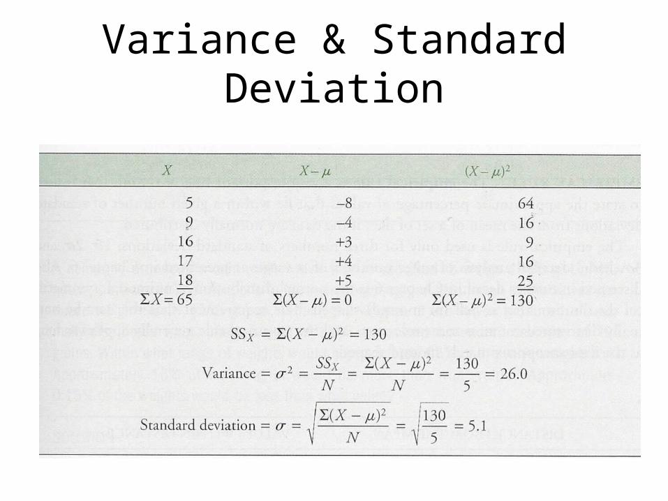
Variance & Standard Deviation

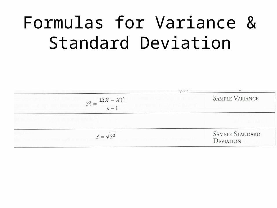
Formulas for Variance & Standard Deviation

1.Age

4.Study / Week (hrs)

5. Auto Cost

($)

6.Alch bev /

wk (#)

7.Sodas / wk (#)

8.Hrs. Paid / wk (hrs)

9.No. units this sem

(#)

10.TV /

video game /

wk (hrs)

11.Movie

theater / wk (#)

12.$/wk

entertain ($)

Mean 20.61 13.67 21303.45 8.83 3.56 9.53 16.56 7.41 5.47 46.41Standard Error 0.552 1.165 2971.803 1.957 0.798 2.140 0.359 0.917 0.831 6.335Median 20 12.5 18000 6 2 4.5 16 5 3.5 40Mode 19 10 18000 0 0 0 16 4 3 100Standard Deviation 3.172 6.693 16003.649 11.071 4.584 12.105 2.061 5.269 4.775 35.836Sample Variance 10.059 44.792 256116773.399 122.558 21.012 146.531 4.246 27.757 22.796 1284.249Kurtosis 7.659 1.160 1.750 5.879 4.415 0.969 2.604 0.072 3.973 0.840Skewness 2.663 1.123 1.320 2.242 1.967 1.291 0.983 1.020 2.046 1.091Range 15 28 65000 50 20 40 10 18 20 150Minimum 18 5 1000 0 0 0 13 2 0 0Maximum 33 33 66000 50 20 40 23 20 20 150Sum 680 451 617800 282.5 117.5 305 546.5 244.5 180.5 1485Count 33 33 29 32 33 32 33 33 33 32Largest(1) 33 33 66000 50 20 40 23 20 20 150Smallest(1) 18 5 1000 0 0 0 13 2 0 0

Empirical Rule

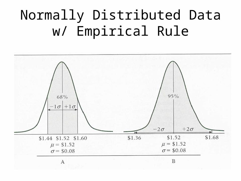
Normally Distributed Data w/ Empirical Rule

Example: Empirical Rule

A company produces a lightweight valve that is specified to weigh 1365 g.

Unfortunately, because of imperfections in the manufacturing process not all of the valves produced weigh exactly 1365 grams.

In fact, the weights of the valves produced are normally distributed with a mean weight of 1365 grams and a standard deviation of 294 grams.

Question?

1) Within what range of weights would approximately 95% of the valve weights fall?

2) Approximately 16% of the weights would be more than what value?

3) Approximately 0.15% of the weights would be less than what value?

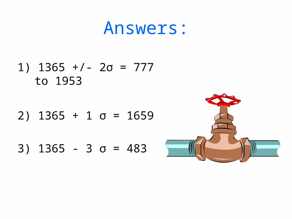
Answers:

1) 1365 +/- 2σ = 777 to 1953

2) 1365 + 1 σ = 1659

3) 1365 - 3 σ = 483

Example 2: Standard Deviation & the Empirical Rule

A recent report states that for California the average statewide price of a gallon of regular gasoline is $1.52.

Suppose regular gas prices vary across the state with a standard deviation of $0.08 are normally distributed.

With x-bar = $1.52 & s = $0.08

1) Nearly all gas prices (97.7%) should fall between what prices?

2) Approximately 16% of the gas prices should be less than what price?

3) Approximately 2.5% of the gas prices should be more than what price?

Answers:

1) µ +/- 3σ = $1.28 and $1.76

2) $1.44 (Since 68% of the prices lie w/in 1σ of the mean, 32% lie outside this range: 16% in each tail.

3) $1.68 (Since 95% of the price lie w/in 2 σ of the mean, 5% lie outside this range: 2.5% in each tail.

Coefficient of Variation

Compares the variation between

two data sets with different means

and different standard deviations

and measures the variation in

relative terms.

Coefficient of Variation (CV) formula

CV = σ / µ (100)

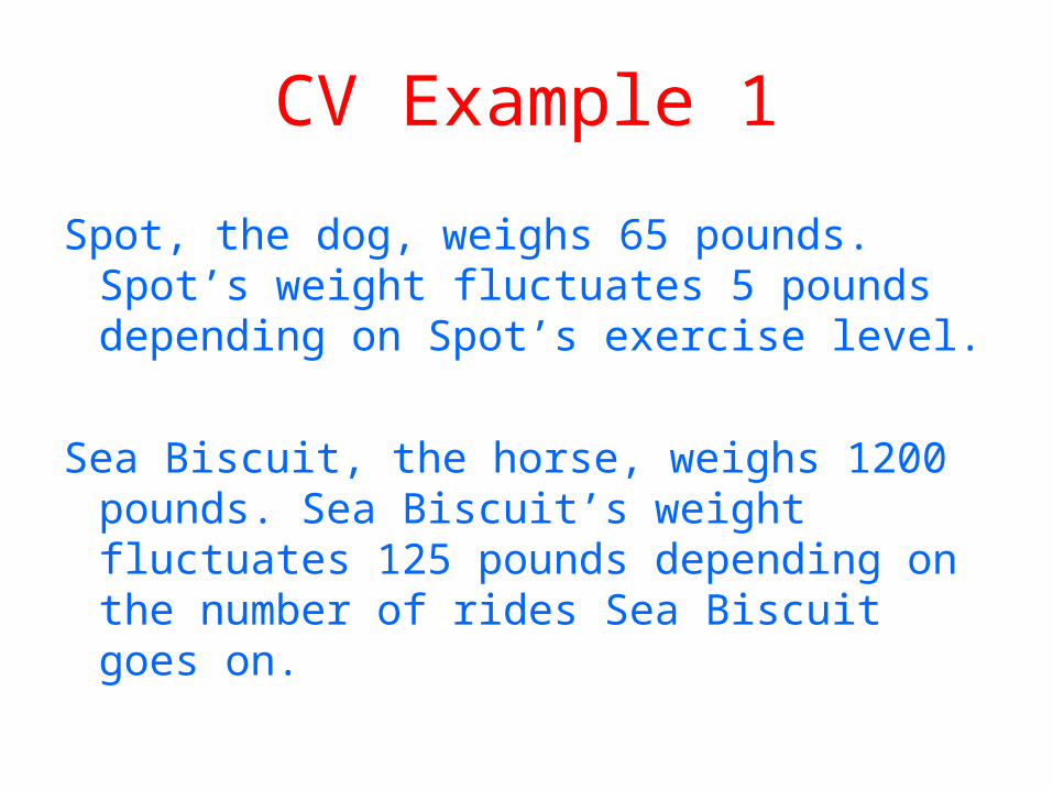
CV Example 1

Spot, the dog, weighs 65 pounds. Spot’s weight fluctuates 5 pounds depending on Spot’s exercise level.

Sea Biscuit, the horse, weighs 1200 pounds. Sea Biscuit’s weight fluctuates 125 pounds depending on the number of rides Sea Biscuit goes on.

Question?

Relatively speaking, which animal’s weight, Spot or Sea Biscuit’s, varies the most?

Coefficient of Variation vs. Standard Deviation

Some financial investors use the coefficient of variation or the standard deviation or both as measures of risk.

What does the Coefficient of Variation tell us about the risk of a stock that the standard deviation

does not?

Relative to the amount invested in a stock, the coefficient of variation reveals the risk of a stock in terms of the size of standard deviation

relative to the size of the mean (in percentage).

CV Example 2:

SUPPOSE:

Five weeks of average prices for stock A are:

$57, $68, $64, $71, and $62.

While five weeks of average prices for stock B are:

$12, $17, $8, $15, and $13.

QUESTION:

Relative to the amount of money invested in the stock, which stock, A or B, is riskier?

Stock A vs. Stock B in terms of Risk

Stock A

µ = 64.40

σ = 4.84

CV = σ/ µ (100) = 7.5%

Stock B

µ = 13

σ = 3.03

CV = σ/ µ (100) = 23.3%

Measures of Position

Indicate how a particular value fits in with all the other data values.

Commonly used measures of position are:

PercentilesQuartiles

Z-scores

TO FIND THE LOCATION OF THE Pth PERCENTILE:

• Determine n ∙ P /100 and use one of the following two location rules:

• Location rule 1. If n ∙ P /100 is NOT a counting number, round up, and the Pth percentile will be the value in this position of the ordered data.

• Location rule 2. If n ∙ P /100 is a counting number, the Pth percentile is the average of the number in this location (of the ordered data) and the number in the next largest location.

Use the two rules of percentiles and the following data to determine both the 85th and the 50th

percentile for starting salary.

Starting Salary Data: 3130 2940 2920 2710 2850 2880 2755 3050 2880 3325 2950 2890

2710 2755 2850 2880 2880 2890 2920 2940 2950 3050 3130 3325

Step 1: Arrange the data in ascending order

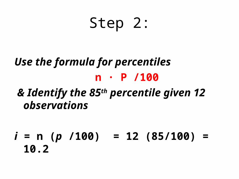
Step 2:

Use the formula for percentiles

n ∙ P /100

& Identify the 85th percentile given 12 observations

i = n (p /100) = 12 (85/100) = 10.2

Because i is not an integer, round up.

The position of the 85th percentile is the next integer greater than 10.2, the

11th position.

2710 2755 2850 2880 2880 2890 2920 2940 2950 3050 3130 3325

From the data, the 85th percentile is the value in the 11th position, or $3130.

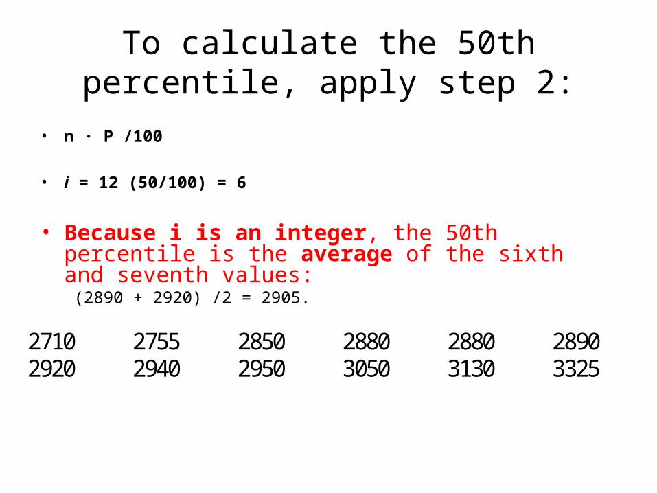
To calculate the 50th percentile, apply step 2:

• n ∙ P /100

• i = 12 (50/100) = 6

• Because i is an integer, the 50th percentile is the average of the sixth and seventh values: (2890 + 2920) /2 = 2905.

2710 2755 2850 2880 2880 2890 2920 2940 2950 3050 3130 3325

Quartiles• Quartiles are merely particular percentiles that

divide the data into quarters:

• Q1 = 1st quartile = 25th percentile (P25)• Q2 = 2nd quartile = 50th percentile

(P50)• Q3 = 3rd quartile = 75th percentile (P75)

• Quartiles are used as benchmarks, much like the use of A,B,C,D, and F on exam grades.

Z- Scores

A z-score determines the relative position of any particular data value x, and is expressed in terms of the number of standard deviations above or below the mean.

Measures of Shape

Measures of shape address skewness and kurtosis.

Skewness• Symmetric data = the sample mean =

sample median

• Right-skewed (positive) = mean > median

• Left-skewed (negative) = mean < median

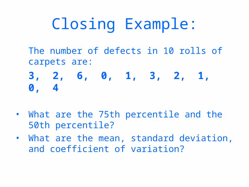
Closing Example:

The number of defects in 10 rolls of carpets are:

3, 2, 6, 0, 1, 3, 2, 1, 0, 4

• What are the 75th percentile and the 50th percentile?

• What are the mean, standard deviation, and coefficient of variation?