Chapter 3

Evaluating Properties

Learning Outcomes ► Demonstrate understanding of key

concepts . . . including phase and pure substance, state principle for simple compressible systems, p-v and T-v graphs, saturation temperature and saturation pressure, two-phase liquid-vapor mixture, quality, enthalpy, and specific heats.

► Apply energy balance with property data.

Learning Outcomes, cont.

► Locate states on p-v, T-v and other thermodynamic diagrams T-h, for example.

► Retrieve property data from Tables A-1 through A-23.

► Apply the ideal gas model for thermo-dynamic analysis, including determining when use of the model is warranted.

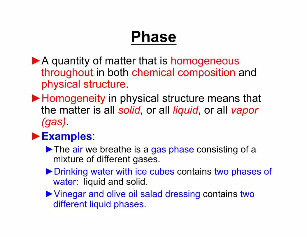
Phase ► A quantity of matter that is homogeneous

throughout in both chemical composition and physical structure.

► Homogeneity in physical structure means that the matter is all solid, or all liquid, or all vapor (gas).

► Examples: ► The air we breathe is a gas phase consisting of a

mixture of different gases. ► Drinking water with ice cubes contains two phases of

water: liquid and solid. ► Vinegar and olive oil salad dressing contains two

different liquid phases.

Pure Substance ► A substance that is uniform and invariable

in chemical composition. ► A pure substance can exist in more than

one phase, but its chemical composition must be the same in each phase.

► Examples: ► Drinking water with ice cubes can be regarded

as a pure substance because each phase has the same composition.

► A fuel-air mixture in the cylinder of an automobile engine can be regarded as a pure substance until ignition occurs.

State Principle for Simple Compressible Systems

► Not all of the relevant intensive properties are independent. ► Some are related by definitions – for example,

density is 1/v and specific enthalpy is u + pv (Eq. 3.4).

► Others are related through expressions developed from experimental data.

► Some intensive properties may be independent in a single phase, but become dependent when there is more than one phase present.

State Principle for Simple Compressible Systems

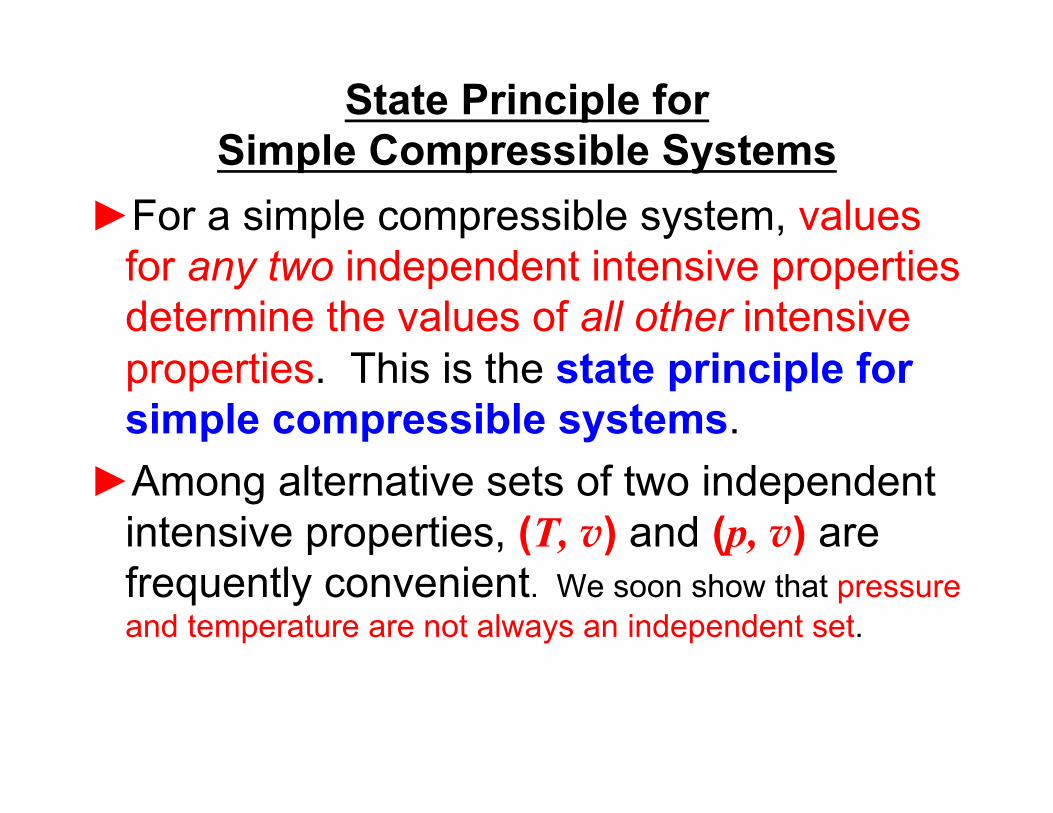
► For a simple compressible system, values for any two independent intensive properties determine the values of all other intensive properties. This is the state principle for simple compressible systems.

► Among alternative sets of two independent intensive properties, (T, v) and (p, v) are frequently convenient. We soon show that pressure and temperature are not always an independent set.

Phase Change ► Consider a closed system consisting of a unit mass of

liquid water at 20oC contained within a piston-cylinder assembly.

► This state is represented by l (highlighted by the blue dot).

► Liquid states such as this, where temperature is lower than the saturation temperature corresponding to the pressure at the state, are called compressed liquid states.

● l

Saturated Liquid ► As the system is heated at constant pressure, the

temperature increases considerably while the specific volume increases slightly.

► Eventually, the system is brought to the state represented by f (highlighted by the blue dot).

► This is the saturated liquid state corresponding to the specified pressure.

● f

Two-Phase Liquid-Vapor Mixture ► When the system is at the saturated liquid state,

additional heat transfer at fixed pressure results in the formation of vapor without change in temperature but with a considerable increase in specific volume as shown by movement of the blue dot.

► With additional heating at fixed pressure, more vapor is formed and specific volume increases further as shown by additional movement of the blue dot.

● f ●

► At these states, the system now consists of a two-phase liquid-vapor mixture.

Two-Phase Liquid-Vapor Mixture ► When a mixture of liquid and vapor exists in equilibrium,

the liquid phase is a saturated liquid and the vapor phase is a saturated vapor.

► For a two-phase liquid-vapor mixture, the ratio of the mass of vapor present to the total mass of the mixture is its quality, x.

●

vaporliquid

vapor

mmm

x+

=► The value of quality ranges from 0 to 1.

► At saturated liquid states, x = 0.

Saturated Vapor ► If the system is heated further until the last bit of

liquid has vaporized it is brought to the saturated vapor state.

► This state is represented by g (highlighted by the blue dot).

► At saturated vapor states, x = 1.

● g

Superheated Vapor ► When the system is at the saturated vapor state, further

heating at fixed pressure results in increases in both temperature and specific volume.

► This state is represented by s (highlighted by the blue dot). ► Vapor states such as this, where temperature is higher than

the saturation temperature corresponding to the pressure at the state, are called superheated vapor states.

● s

Steam Tables ► Tables of properties for different substances

are frequently set up in the same general format. The tables for water, called the steam tables, provide an example of this format. The steam tables are in appendix tables A-2 through A-5. ► Table A-4 applies to water as a superheated

vapor. ► Table A-5 applies to compressed liquid water. ► Tables A-2 and A-3 apply to the two-phase,

liquid-vapor mixture of water.

T oC

v m3/kg

u kJ/kg

h kJ/kg

s kJ/kg·K

v m3/kg

u kJ/kg

h kJ/kg

s kJ/kg·K

p = 80 bar = 8.0 MPa

(Tsat = 295.06oC)

p = 100 bar = 10.0 MPa (Tsat = 311.06oC)

Sat. 0.02352 2569.8 2758.0 5.7432 0.01803 2544.4 2724.7 5.6141 320 0.02682 2662.7 2877.2 5.9489 0.01925 2588.8 2781.3 5.7103 360 0.03089 2772.7 3019.8 6.1819 0.02331 2729.1 2962.1 6.0060 400 0.03432 2863.8 3138.3 6.3634 0.02641 2832.4 3096.5 6.2120 440 0.03742 2946.7 3246.1 6.5190 0.02911 2922.1 3213.2 6.3805 480 0.04034 3025.7 3348.4 6.6586 0.03160 3005.4 3321.4 6.5282

Single-Phase Regions ► Example: Properties associated with superheated

water vapor at 10 MPa and 400oC are found in Table A-4. ► v = 0.02641 m3/kg ► u = 2832.4 kJ/kg

Table A-4

► h = 3096.5 kJ/kg ► s = 6.2120 kJ/kg·K

Linear Interpolation ► When a state does not fall exactly on the grid of values provided

by property tables, linear interpolation between adjacent entries is used.

► Example: Specific volume (v) associated with superheated water vapor at 10 bar and 215oC is found by linear interpolation between adjacent entries in Table A-4.

T oC

v m3/kg

u kJ/kg

h kJ/kg

s kJ/kg·K

p = 10 bar = 1.0 MPa

(Tsat = 179.91oC)

Sat. 0.1944 2583.6 2778.1 6.5865 200 0.2060 2621.9 2827.9 6.6940 240 0.2275 2692.9 2920.4 6.8817

Table A-4

(0.2275 – 0.2060) m3/kg (v – 0.2060) m3/kg (240 – 200)oC (215 – 200)oC

slope = = → v = 0.2141 m3/kg

Two-Phase Liquid-Vapor Region ► Tables A-2/A-2E

(Temperature Table) and A-3/A-3E (Pressure Table) provide ► saturated liquid (f) data ► saturated vapor (g) data

Specific Volume m3/kg

Internal Energy kJ/kg

Enthalpy kJ/kg

Entropy kJ/kg·K

Temp oC

Press. bar

Sat. Liquid

vf×103

Sat. Vapor

vg

Sat. Liquid

uf

Sat. Vapor

ug

Sat. Liquid

hf

Evap.

hfg

Sat. Vapor

hg

Sat. Liquid

sf

Sat. Vapor

sg

Temp oC

.01 0.00611 1.0002 206.136 0.00 2375.3 0.01 2501.3 2501.4 0.0000 9.1562 .01 4 0.00813 1.0001 157.232 16.77 2380.9 16.78 2491.9 2508.7 0.0610 9.0514 4 5 0.00872 1.0001 147.120 20.97 2382.3 20.98 2489.6 2510.6 0.0761 9.0257 5 6 0.00935 1.0001 137.734 25.19 2383.6 25.20 2487.2 2512.4 0.0912 9.0003 6 8 0.01072 1.0002 120.917 33.59 2386.4 33.60 2482.5 2516.1 0.1212 8.9501 8

Table A-2

Table note: For saturated liquid specific volume, the table heading is vf×103. At 8oC, vf × 103 = 1.002 → vf = 1.002/103 = 1.002 × 10–3.

► The specific volume of a two-phase liquid- vapor mixture can be determined by using the saturation tables and quality, x.

► The total volume of the mixture is the sum of the volumes of the liquid and vapor phases:

Two-Phase Liquid-Vapor Region

V = Vliq + Vvap

► Dividing by the total mass of the mixture, m, an average specific volume for the mixture is:

mV

mV

mV vapliq

+==v

► With Vliq = mliqvf , Vvap = mvapvg , mvap/m = x , and mliq/m = 1 – x :

v = (1 – x)vf + xvg = vf + x(vg – vf) (Eq. 3.2)

Two-Phase Liquid-Vapor Region ► Since pressure and temperature are NOT

independent properties in the two-phase liquid-vapor region, they cannot be used to fix the state in this region.

► The property, quality (x), defined only in the two-phase liquid-vapor region, and either temperature or pressure can be used to fix the state in this region.

v = (1 – x)vf + xvg = vf + x(vg – vf) (Eq. 3.2) u = (1 – x)uf + xug = uf + x(ug – uf) (Eq. 3.6) h = (1 – x)hf + xhg = hf + x(hg – hf) (Eq. 3.7)

Two-Phase Liquid-Vapor Region ► Example: A system consists of a two-phase liquid-vapor

mixture of water at 6oC and a quality of 0.4. Determine the specific volume, in m3/kg, of the mixture.

► Solution: Apply Eq. 3.2, v = vf + x(vg – vf)

Specific Volume m3/kg

Internal Energy kJ/kg

Enthalpy kJ/kg

Entropy kJ/kg·K

Temp oC

Press. bar

Sat. Liquid

vf×103

Sat. Vapor

vg

Sat. Liquid

uf

Sat. Vapor

ug

Sat. Liquid

hf

Evap.

hfg

Sat. Vapor

hg

Sat. Liquid

sf

Sat. Vapor

sg

Temp oC

.01 0.00611 1.0002 206.136 0.00 2375.3 0.01 2501.3 2501.4 0.0000 9.1562 .01 4 0.00813 1.0001 157.232 16.77 2380.9 16.78 2491.9 2508.7 0.0610 9.0514 4 5 0.00872 1.0001 147.120 20.97 2382.3 20.98 2489.6 2510.6 0.0761 9.0257 5 6 0.00935 1.0001 137.734 25.19 2383.6 25.20 2487.2 2512.4 0.0912 9.0003 6 8 0.01072 1.0002 120.917 33.59 2386.4 33.60 2482.5 2516.1 0.1212 8.9501 8

Table A-2

Substituting values from Table 2: vf = 1.001×10–3 m3/kg and vg = 137.734 m3/kg:

v = 1.001×10–3 m3/kg + 0.4(137.734 – 1.001×10–3) m3/kg v = 55.094 m3/kg

Property Data Use in the Closed System Energy Balance

Example: A piston-cylinder assembly contains 2 kg of water at 100oC and 1 bar. The water is compressed to a saturated vapor state where the pressure is 2.5 bar. During compression, there is a heat transfer of energy from the water to its surroundings having a magnitude of 250 kJ. Neglecting changes in kinetic energy and potential energy, determine the work, in kJ, for the process of the water.

State 1 2 kg

of water T1 = 100oC p1 = 1 bar

State 2 Saturated vapor p2 = 2.5 bar

Q = –250 kJ

2 ● ●

T

v

p1 = 1 bar

1

p2 = 2.5 bar

T1 = 100oC

Property Data Use in the Closed System Energy Balance

Solution: An energy balance for the closed system is

ΔKE + ΔPE +ΔU = Q – W 0 0

where the kinetic and potential energy changes are neglected.

Thus W = Q – m(u2 – u1)

State 1 is in the superheated vapor region and is fixed by p1 = 1 bar and T1 = 100oC. From Table A-4, u1 = 2506.7 kJ/kg.

State 2 is saturated vapor at p2 = 2.5 bar. From Table A-3, u2 = ug = 2537.2 kJ/kg.

W = –250 kJ – (2 kg)(2537.2 – 2506.7) kJ/kg = –311 kJ

The negative sign indicates work is done on the system as expected for a compression process.

Specific Heats ► Three properties related to specific internal energy and specific

enthalpy having important applications are the specific heats cv and cp and the specific heat ratio k.

vv ⎟

⎠

⎞⎜⎝

⎛∂

∂=

Tuc

(Eq. 3.8) p

p Thc ⎟⎠

⎞⎜⎝

⎛∂

∂=

(Eq. 3.9) vcc

k p=

(Eq. 3.10)

►  In general, cv is a function of v and T (or p and T), and cp depends on both p and T (or v and T).

► Specific heat data are provided in Fig 3.9 and Tables A-19 through A-21.

Property Approximations for Liquids ► Approximate values for v, u, and h at liquid states can be

obtained using saturated liquid data. ► Since the values of v and u for liquids

change very little with pressure at a fixed temperature, Eqs. 3.11 and 3.12 can be used to approximate their values.

v(T, p) ≈ vf(T) u(T, p) ≈ uf(T)

(Eq. 3.11) (Eq. 3.12)

► An approximate value for h at liquid states can be obtained using Eqs. 3.11 and 3.12 in the definition h = u + pv: h(T, p) ≈ uf(T) + pvf(T) or alternatively h(T, p) ≈ hf(T) + vf(T)[p – psat(T)] (Eq. 3.13) where psat denotes the saturation pressure at the given temperature

► When the underlined term in Eq. 3.13 is small h(T, p) ≈ hf(T) (Eq. 3.14)

Saturated liquid

Incompressible Substance Model ► For a substance modeled as incompressible

► v = constant

► For a substance modeled as incompressible, cp = cv; the common specific heat value is represented by c.

► For a substance modeled as incompressible with constant c:

u2 – u1 = c(T2 – T1) (Eq. 3.20a) h2 – h1 = c(T2 – T1) + v(p2 – p1) (Eq. 3.20b)

► In Eq. 3.20b, the contribution of the underlined term is often small enough to be ignored.

► u = u(T)

Generalized Compressibility Chart v► The p- -T relation for 10 common gases is

shown in the generalized compressibility chart.

Generalized Compressibility Chart

TRpZ v

=

► In this chart, the compressibility factor, Z, is plotted versus the reduced pressure, pR, and reduced temperature TR, where

pR = p/pc TR = T/Tc

(Eq. 3.27) (Eq. 3.28) (Eq. 3.23)

The symbols pc and Tc denote the temperature and pressure at the critical point for the particular gas under consideration. These values are obtained from Tables A-1 and A-1E.

R8.314 kJ/kmol·K 1.986 Btu/lbmol·oR 1545 ft·lbf/lbmol·oR

(Eq. 3.22)

is the universal gas constant

=R

Studying the Generalized Compressibility Chart

► Low values of pR, where Z ≈ 1, do not necessarily correspond to a range of low absolute pressures.

► For instance, if pR = 0.10, then p = 0.10pc. With pc values from Table A-1

► These pressure values range from 3.8 to 22 bar, which in engineering practice are not normally considered as low pressures.

Water vapor pc = 220.9 bar → p = 22 bar Ammonia pc = 112.8 bar → p = 11.2 bar Carbon dioxide pc = 73.9 bar → p = 7.4 bar Air pc = 37.7 bar → p = 3.8 bar

Introducing the Ideal Gas Model

► To recap, the generalized compressibility chart shows that at states where the pressure p is small relative to the critical pressure pc (where pR is small), the compressibility factor Z is approximately 1.

► At such states, it can be assumed with reasonable accuracy that Z = 1. Then

pv = RT (Eq. 3.32)

Introducing the Ideal Gas Model

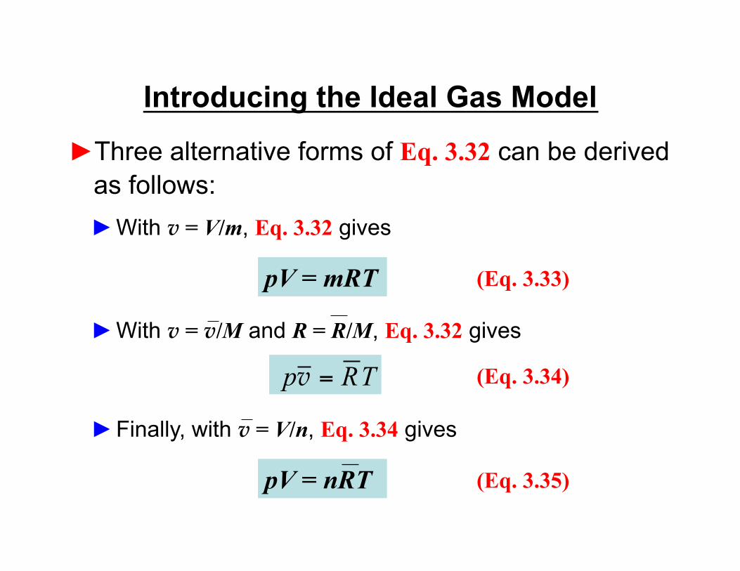
► Three alternative forms of Eq. 3.32 can be derived as follows: ► With v = V/m, Eq. 3.32 gives

pV = mRT (Eq. 3.33)

► With v = v/M and R = R/M, Eq. 3.32 gives

(Eq. 3.34) TRp =v

► Finally, with v = V/n, Eq. 3.34 gives

pV = nRT (Eq. 3.35)

Introducing the Ideal Gas Model ► Investigation of gas behavior at states where Eqs.

3.32-3.35 are applicable indicates that the specific internal energy depends primarily on temperature. Accordingly, at such states, it can be assumed with reasonable accuracy that it depends on temperature alone:

u = u(T) (Eq. 3.36)

► With Eqs. 3.32 and 3.36, the specific enthalpy also depends on temperature alone at such states:

h = u + pv = u(T) + RT (Eq. 3.37)

► Collecting results, a gas modeled as an ideal gas adheres to Eqs. 3.32-3.35 and Eqs. 3.36 and 3.37.

Introducing the Ideal Gas Model ► While the ideal gas model does not provide an

acceptable approximations throughout, in most commonly applied engineering situations it is justified for use.

► Appropriateness of the ideal gas model can be

checked by locating states under consideration on one of the generalized compressibility charts provided by appendix figures Figs. A-1 through A-3.

Internal Energy and Enthalpy of Ideal Gases

► For a gas obeying the ideal gas model, specific internal energy depends only on temperature. Hence, the specific heat cv, defined by Eq. 3.8, is also a function of temperature alone. That is,

(Eq. 3.38) dTduTc =)(v (ideal gas)

► On integration,

(Eq. 3.40) ( ) ( ) dTTcTuTu ∫=− )(12 vT1

T2

(ideal gas)

Internal Energy and Enthalpy of Ideal Gases

► Similarly, for a gas obeying the ideal gas model, specific enthalpy depends only on temperature. Hence, the specific heat cp, defined by Eq. 3.9, is also a function of temperature alone. That is,

(Eq. 3.41) dTdhTcp =)( (ideal gas)

► On integration,

(Eq. 3.43) ( ) ( ) dTTcThTh p∫=− )(12T1

T2

(ideal gas)

Internal Energy and Enthalpy of Ideal Gases

► In applications where the specific heats are modeled as constant,

► For several common gases, evaluation of changes in specific internal energy and enthalpy is facilitated by use of the ideal gas tables: Tables A-22 and A-23.

► Table A-22 applies to air modeled as an ideal gas.

(Eq. 3.50) (Eq. 3.51)

u(T2) – u(T1) = cv[T2 – T1] h(T2) – h(T1) = cp[T2 – T1]

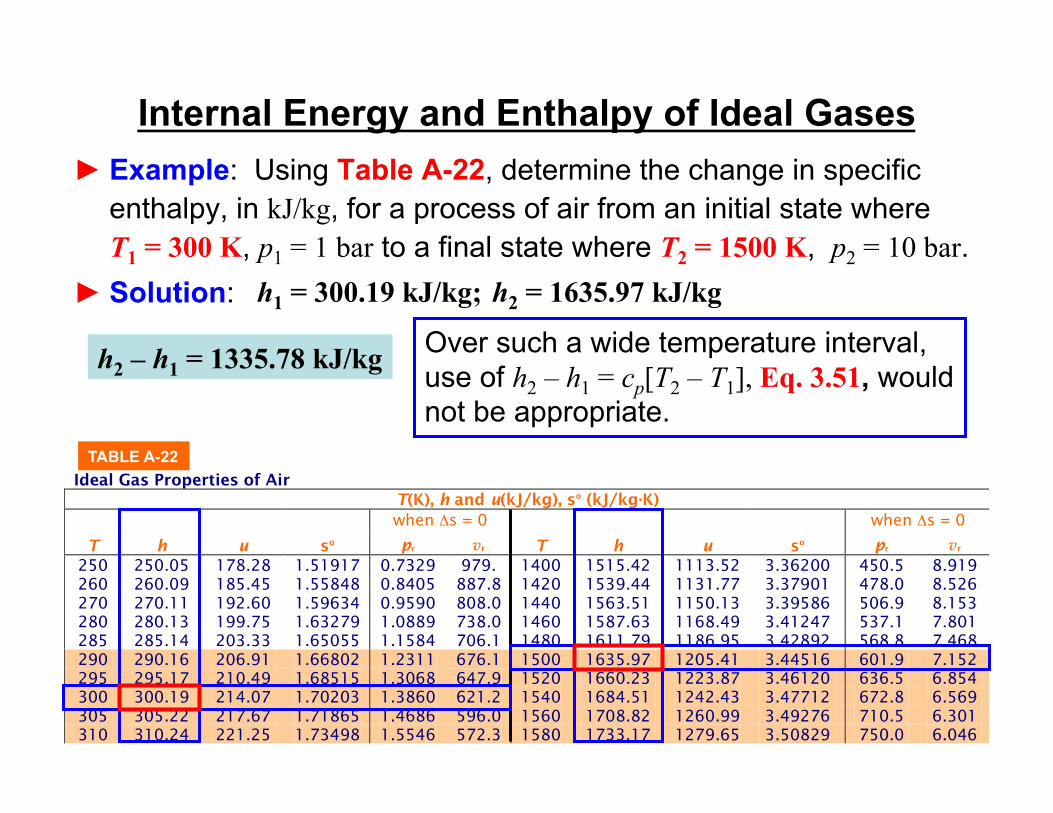
TABLE A-22 Ideal Gas Properties of Air

T(K), h and u(kJ/kg), so (kJ/kg·K) when Δs = 0 when Δs = 0

T h u so pr vr T h u so pr vr 250 250.05 178.28 1.51917 0.7329 979. 1400 1515.42 1113.52 3.36200 450.5 8.919 260 260.09 185.45 1.55848 0.8405 887.8 1420 1539.44 1131.77 3.37901 478.0 8.526 270 270.11 192.60 1.59634 0.9590 808.0 1440 1563.51 1150.13 3.39586 506.9 8.153 280 280.13 199.75 1.63279 1.0889 738.0 1460 1587.63 1168.49 3.41247 537.1 7.801 285 285.14 203.33 1.65055 1.1584 706.1 1480 1611.79 1186.95 3.42892 568.8 7.468 290 290.16 206.91 1.66802 1.2311 676.1 1500 1635.97 1205.41 3.44516 601.9 7.152 295 295.17 210.49 1.68515 1.3068 647.9 1520 1660.23 1223.87 3.46120 636.5 6.854 300 300.19 214.07 1.70203 1.3860 621.2 1540 1684.51 1242.43 3.47712 672.8 6.569 305 305.22 217.67 1.71865 1.4686 596.0 1560 1708.82 1260.99 3.49276 710.5 6.301 310 310.24 221.25 1.73498 1.5546 572.3 1580 1733.17 1279.65 3.50829 750.0 6.046

Internal Energy and Enthalpy of Ideal Gases ► Example: Using Table A-22, determine the change in specific

enthalpy, in kJ/kg, for a process of air from an initial state where T1 = 300 K, p1 = 1 bar to a final state where T2 = 1500 K, p2 = 10 bar.

► Solution: h1 = 300.19 kJ/kg; h2 = 1635.97 kJ/kg

h2 – h1 = 1335.78 kJ/kg Over such a wide temperature interval, use of h2 – h1 = cp[T2 – T1], Eq. 3.51, would not be appropriate.

Property Data Use in the Closed System Energy Balance

Example: A closed, rigid tank consists of 1 kg of air at 300 K. The air is heated until its temperature becomes 1500 K. Neglecting changes in kinetic energy and potential energy and modeling air as an ideal gas, determine the heat transfer, in kJ, during the process of the air.

1 kg of air

Q

T1 = 300 K T2 = 1500 K State 1 State 2

2 ●

●

T

v

T1 = 300 K 1

T2 = 1500 K

p2

p1

Property Data Use in the Closed System Energy Balance

Solution: An energy balance for the closed system is

ΔKE + ΔPE +ΔU = Q – W 0 0 0

where the kinetic and potential energy changes are neglected and W = 0 because there is no work mode.

Thus Q = m(u2 – u1)

TABLE A-22 Ideal Gas Properties of Air

T(K), h and u(kJ/kg), so (kJ/kg·K) when Δs = 0 when Δs = 0

T h u so pr vr T h u so pr vr 250 250.05 178.28 1.51917 0.7329 979. 1400 1515.42 1113.52 3.36200 450.5 8.919 260 260.09 185.45 1.55848 0.8405 887.8 1420 1539.44 1131.77 3.37901 478.0 8.526 270 270.11 192.60 1.59634 0.9590 808.0 1440 1563.51 1150.13 3.39586 506.9 8.153 280 280.13 199.75 1.63279 1.0889 738.0 1460 1587.63 1168.49 3.41247 537.1 7.801 285 285.14 203.33 1.65055 1.1584 706.1 1480 1611.79 1186.95 3.42892 568.8 7.468 290 290.16 206.91 1.66802 1.2311 676.1 1500 1635.97 1205.41 3.44516 601.9 7.152 295 295.17 210.49 1.68515 1.3068 647.9 1520 1660.23 1223.87 3.46120 636.5 6.854 300 300.19 214.07 1.70203 1.3860 621.2 1540 1684.51 1242.43 3.47712 672.8 6.569 305 305.22 217.67 1.71865 1.4686 596.0 1560 1708.82 1260.99 3.49276 710.5 6.301 310 310.24 221.25 1.73498 1.5546 572.3 1580 1733.17 1279.65 3.50829 750.0 6.046

Q = (1 kg)(1205.41 – 214.07) kJ/kg = 991.34 kJ

Substituting values for specific internal energy from Table A-22

(Eq. 3.52)

Polytropic Process ► A polytropic process is a quasiequilibrium process

described by pV

n = constant

► The exponent, n, may take on any value from –∞ to +∞ depending on the particular process.

► For any gas (or liquid), when n = 0, the process is a constant-pressure (isobaric) process. ► For any gas (or liquid), when n = ±∞, the process is a constant-volume (isometric) process. ► For a gas modeled as an ideal gas, when n = 1, the process is a constant-temperature (isothermal) process.