CHAPTER IV PREDICTABILITY OF THE BS MODEL IN INDIAN

99

CHAPTER IV

Asset pricing model should predict its price correctly as that of the

market and the residuals / error shoul systematic pattern with

any of its variables / parameters that ar

changes systematically with the change in variables then it is known as bias of

the model. The residuals should be distributed normally. This chapter explains

the predictability of the model and behaviour of th ption towards its

variables li ,

of returns of the stock, exercise price, and risk-free interest rate. The findings of

the study are explained in depth. Part research study was published in

the book “ Manage t Pra Polic Princ [105], by

The Allied Publishers Private Limited, New Delhi, after edited by a faculty of

Indian Inst agem dore xure

4.2 EARL DIE Bla stat mar s of tions “t differ in

certain sys ys” fr val by model tions with

less than hs to tion optio are ei eep in or

out of the rton ates est all pri r deep in

the money dee f th opt less t e market

prices. M and Mervil 4] op deep mone ons have

model prices those are lower than market prices, whereas deep out of money

options

PREDICTABILITY OF THE BS MODEL IN INDIAN OPTION MARKET

4.1 INTRODUCTION

d not have any

e used to predict the price. If the error

e call o prices

ke stock price and life of the option and the parameters like volatility

of this

Business men ctices, ies and iples”

itute of Man ent, In . (Anne I)

IER STU S

ck [21, 23] es that ket price call op end to

tematic wa om the ues given the BS for op

three mont expira and for ns that ther d

money. Me [98] st that BS imated c ces fo

as well as p out o e money ions are han th

acbeth le [9 ine that in the y opti

have model prices that are higher. These conflicts may perhaps be

100

reconciled by the fact that the studies examined market prices at different points

in time and these systematic biases vary with time (Rubinstein [41,118]).

4.3 DEFINITIONS

Based on the above studies, this research tries to find the truth about

the predictability of the BS Model and pricing biases, if any, in the Indian option

market. The Mean Absolute Errors (MAE) calculated with the following formula

for various moneyness and various lives of the options are tabulated in the

Table 4.1.

Σ ׀ PO – PT׀ Mean Absolute Error = ------------------- Σ PO

where PT is the call option price theoretically calculated using BS model and PO

is the observed call option prices in the market.

Moneyness is defined as S0 / X and the values ranging 0.99 to 1.01 are

taken as at-the-money options, values les ed as out-of-

the-money options and above 1.01 as in-the-money options. As the number is

increasing the mo

Mean percentage errors are calculated using the following formula.

[{(PO – PT) / P ] Mean Percentage Er -------------- n

where n is the sample

The percentage he formu O – PT) / PO} x100] in

each of the options taken in the sample. Then, the sum of the percentage errors

is calculated and result is divided by the number of data “n”.

s than 0.99 is consider

neyness is also increasing.

Σror = -----------------

O} x100

size.

error is found using t la [{(P

101

Though the mean percentage error is misrepresenting in the cases of

very low option prices, it gives irection of the err enlighten us whether,

the BS model is overpricing or under-pricing the options. Thus it is considered

the research studies abroad are not

considering the deep out-of-the-money options and deep in-the-money options,

ut, they have so little data that they

cannot predict the market price correctly. If the data volume is not sufficient

the d or. It

as an important measure and used in the research.

4.4 CLASSIFICATION OF DATA

First, the call options that are offered by NSE were collected, analyzed

and the traded options were segregated from the non-traded ones. Then, using

the ex-dividend dates and dates of board meetings related to dividend

decisions, the options related to cum-dividend stocks during the life of the

options were eliminated. Lastly, the data are classified into fourteen groups of

moneyness each having three consecutive classes of moneyness. The

definition of moneyness is So / X. The classifications started from 0.83 to 1.20.

The classification is made in a way that ATM options of 1.00 lies at the center of

the classification (0.99 to 1.01). Though,

they have also studied in Indian context. B

enough they are not considered for making conclusion. The details are given in

Table no. 4.1

102

TABLE 4.1

DETAILS OF CALL OPTION TAKEN AS SAMPLE AS PER MONEYNESS

Moneyness S0 / X No. of Data

< 0.83 188 0.84 – 0.86 377 0.87 – 0.89 1,028 0.90 – 0.92 3,204 0.93 – 0.95 8,760 0.96 51 – 0.98 17,20.99 – 1.01 2,1302 1.02 28 – 1.04 17,7 1.05 – 32 1.07 11,2 1.08 – 4 1.10 6,561.11 – 1 1.13 3,871.14 – 1.16 2,346 1.17 – 1.19 1,383

> 1 5 .20 51TOT 77AL 96,5

t o bov opti a 6 lier been na

the final sample size is 95,956. Box-Plot analysis is used to identify the outliers,

whi exp in detail at chapter 6. The call options with moneyness

between 0.93 and 1.10 are having a reason

related to deep in-the-money and deep ou the

very little number of traded options, for which the market may not correctly price

e options. The distribution of the call options looks like a normal curve, but

Ou f the a e call on dat 21 out s have elimi ted and

ch is lained

able number of data. The other data

t-of- -money options are having

th

having fat tail.

103

CHART 4.1

DISTRIBUTION OF CALL OPTION DATA FOR VARIOUS MONEYNESS

DISTRIBUTION OF CALL OPTIONS

0

5,000

10,000

15,000

20,000

25,000

< 0.

83

0.84

-0.8

6

0.87

-0.8

9

0.90

-0.9

2

0.93

-0.9

5

0.96

-0.9

8

0.99

-1.0

1

1.02

-1.0

4

1.05

-1.0

7

1.08

-1.1

0

1.11

-1.1

3

1.14

-1.1

6

1.17

-1.1

9

> 1.

20

MONEYNESS

NO

. OF

CA

LL O

PTIO

NS

4.5 PREDICTABILITY OF THE MODEL

The main objective of this empirical study is the predictability of the

model. The predictability of the model is verified through mean absolute errors,

ross various

determinants of the call option price.

4.5.1 M

mean percentage error and the distribution of these errors ac

EAN ABSOLUTE ERRORS

The options were classified with different categories of moneyness,

processed and the option prices were calculated using BS model. The actual

markets prices of call options taken from the NSE website [68] were compared

104

with the respective predicted prices by the model and the MAE thus calculated

are summarized and shown in the table no. 4.2.

TE ERRORS OF OPTIONS WITH VARIOUS MONEYNESS

TABLE 4.2 MEAN ABSOLU

Moneyness No. Of data

Total Observed

Price

Total Absolute

Error

Mean Absolute

Error

< 0.83 187 4,130 1,635 0.40

0.84-0.86 370 7,265 3,720 0.51

0.87-0.89 1,005 17,501 9,349 0.53

0.90-0.92 3,163 54,356 28,077 0.52

0.93-0.95 8,671 155,569 66,442 0.43

0.96-0.98 17,112 383,157 127,623 0.33

0.99-1.01 21,984 624,996 154,049 0.25

1.02-1.04 17,643 660,766 114,602 0.17

1.05-1.07 11,191 542,341 70,111 0.13

1.08-1.10 6,550 378,344 45,151 0.12

1.11-1.13 3,854 251,920 26,870 0.11

1.14-1.16 2,328 164,207 16,709 0.10

1.17-1.19 1,383 101,157 11,043 0.11

> 1.20 515 62,963 7,688 0.12

It may be observed from the above table, the MAE are as high as about

0.52 for the deep out-of-the-money options having moneyness 0.80 to 0.92.

Then it starts decreasing at a faster rate. For the moneyness of 0.93-0.95, it

dropped down by about 17% to 0.43 and for the next classification of 0.96-0.98,

it reduced by 23% to 0.33. Then, MAE are reduced by 24%, 32%, 23% and 7%

for next four moneynesses. At the end, it is almost flat.

105

The options that are having number of trades very less during the entire

period of five years and ten months (1716 working days) are illiquid and may

not reflect the correct price of the market. If we neglect the data related to

number of options less th ing the of study7; the MAE vary

from 0.12 to 0.43, with a m The clas tions of data with less than

5000 are shown in shades d not be considered for the conclusion

and are given only for the academic purpose. The mean predictability of the

model is around 76%. Mean is not a resistant summary of statistics and is

drastically influenced by th alues. Because of this, the predictability

of the model is low and the . For th ata without categories the

mean absolute error is 0.25 only. Let us also consider the resistant summary of

median based statistics. sorted in the ascending order. The

percentiles are calculated using SAS; values at t responding percentages

are given in the table no.4.3.

TABLE 4.3

an 5000 dur period

ean of 0.24. sifica

, which nee

e extreme v

error is high e full d

MAE are

he cor

PERCENTILES OF MEAN ABSOLUTE ERRORS

PERCENTILE ABSOLUTE ERRORS

100% 625.0199% 69.5195% 25.390% 15.62

Upper Quartile 75% 7.03Median 50% 3.12

Lower Quar 1.27tile 25%10% 0.475% 0.231% 0.050% 0

-------------------------------------------------------------------------------------------------------7Gurdip Bakshi, Charles Cao, and Zhiwu Chen in their study [10] considered data with

more than 4500 only during the period of 3 years.

106

A percentile8 is the value of a variable below which a certain percent of

observations fall. So the 20th percentile is the value (or score) below which 20

percent of the observations may be found. Fifty percentages of the options are

having MAE less than 3.12. The next 25% of the sample are having MAEs

within 3.12 to 7.03. The next 15%of the options are having errors from 7.03 to

15.62. It means, that the BS model predicted the call option prices with a

minimum accuracy of 84.38% for ninety percentages (86,360 options) of the

sample of 95,956. A very small portion of the options are having higher errors.

Thus, it may be inferred that the BS model is good as far as MAE are

considered. The median based statistics give better picture of the error

n the mean, which is influenced by the extreme values.

rs are considered to nullify the effect of positive and

egative errors canceling each other, thus showing smaller error values. But,

tion of the model errors. The

direction of the errors such as positive and negative errors will enlighten one to

entify

5.4% accuracy. If minutely

looked; the model predicts 50% of opt

and 89.19%. The next 30% options are ving predictability between 72% and

80.58% only. (10th percentile is -38.64 and 90th percentile is 39.76). The

accuracy of the prediction measured and summarized is given in table no. 4.4.

-------- ------- 8Source: (http://en.wikipedia.org/wiki/Percentile

distribution tha

4.5.2 MEAN PERCENTAGE ERRORS

The absolute erro

n

MAE has the disadvantage of not showing the direc

id , whether the model overprices or underprices the options.

The mean percentage errors are calculated and categorized into plus or

minus five percentages and exhibited in the table number 4.4. Let us consider

the resistance summary of median and quartiles. The median of the percentage

errors is 4.6, the lower quartile -10.81 and the upper quartile at 20.34. On an

average the model predicts the call option price by 9

ions with a predictability range 79.64%

ha

-------------------------------------------------------------------------------------------).

107

TABLE 4.4 PERCE E C DEL NTAGE WIS PREDI TABILITY OF THE BS MO

Accuracy Error

Number of

Negative Errors

Number of

Positive Errors

Total Number

of Errors

Cumu Total

Number of

Errors

% of Number

of Errors

Cumu % of

Number of

Errors

95% ± 1 18,305 .08 19.085 7,781 10,524 8,305 1990% ± 1 1 33,257 .58 34.660 5,659 9,293 4,952 1585% ± 1 45,207 .45 47.115 4,420 7,530 11,950 1280% ± 2 54,5410 3,338 5,996 9,334 9.73 56.8475% ± 2 62,1925 2,599 5,052 7,651 7.97 64.8170% ± 3 68,2650 2,026 4,047 6,073 6.33 71.1465% ± 35 9 73,265 .21 76.351,73 3,261 5,000 560% ± 40 77,230 .13 80.481,410 2,555 3,965 455% ± 45 80,474 .38 83.871,119 2,125 3,244 350% ± 5 7 83,065 .70 86.570 93 1,654 2,591 245% ± 5 794 1,330 85,189 .21 88.785 2,124 240% ± 60 713 1,056 1,769 86,958 1.84 90.62

Cumu - Cumulative

Out of 95,956 samples, the BS model has predicted the price with 95%

accuracy in 18,305 options; that is 19.08%. 54,541 options that are 56.84% are

predicted within 20% error. About 71.14% of options are having errors less than

30%. The BS model has predicted more number of options within a reasonable

accuracy and few have large errors. The same is depicted in the chart no.4.2.

108

CHART 4.2

PREDICTABILITY OF THE BS MODEL

0

5,000

10,000

PREDIC ABILITYT

15,000RO

20,000. O

F ER

RS

NO

± 5 ±10

±15

±20

±25

±30

±35

±40

±45

±50

±55

±60

PERCENTAGE ERRORS

4.6 BIASES OF THE MODEL ACROSS MONEYNESS

4.6.1 BIASES OF MEAN ABSOLUTE ERRORS

The plot of MAE should be of a straight line with only random variations.

Refer the table no 4.2 (pp 104); the errors are reducing from 0.43 to 0.12 as the

moneyness increases from 0.93 to 1.10. The MAE are coming down with

increase in moneyness and there is definite pattern against moneyness. That is,

MAE and moneyness is inversely related. The mean of the MAE is 0.25. The

rrors are not at random about the mean error. Hence, the pricing bias of the

model

e

over moneyness is proved beyond doubt.

The MAE corresponding to moneyness with more than 5000 data are

given in the chart no. 4.3

109

CHART 4.3

MEAN ABSOLUTE ERRORS FOR DIFFERENT MONEYNESS AFTER AN 5000 ELIMINATION OF DATA LESS TH

MEAN ABSOLUTE ERROR0.45

S

0.00

0.05

0.10

0.15

0.20

0.25

0.30

0.35

0.40

0.93-0.95 0.96-0.98 0.99-1.01 1.02-1.04 1.05-1.07 1.08-1.10MONEYNES

M A

E

The MAE are not at its minimum at moneyness of 1.00 but at its

minimum for the options at moneyness of 1.08. This is against the findings of

Black, Fisher [23] himself and o of the opinion that BS model

predicts correctly for options at-the-money. But our study is not coinciding with

this, a .08

– 1.10.

4.6.2 EXCE RORS OVER N OF EANS F AB UTE ERRO

If the errors are calculated around the mean of the above MAE, then the

mean error occurs at the moneyness of 1.00 and varies in opposite directions

thers. He is

s per our findings the minimum errors are only at the moneyness of 1

SS ER MEA M O SOLRS

110

as per mon results wn for a tte standing in

table no. 4.5 and char

E 4

EXCESS ERRORS OVER THE MEAN OF MEANS OF ABSOLUTE ERRORS FOR MONEY FOR DATA MORE THAN 5000

eyness. The are sho below be r under

t no. 4.4.

TABL .5

DIFFERENT NESS

Moneyness Excess Error

0.87 - 0.89 0.28

0.90 - 0.92 0.27

0.93 - 0.95 0.18

0.96 - 0.98 0.08

0.99 - 1.01 0.00

1.02 - 1.04 -0.08

1.05 - 1.07 -0.12

1.08 - 1.10 -0.13

1.11 - 1.13 -0.14

1.14 - 1.16 -0.15

1.17 - 1.20 -0.14

ed

areas of the above table. The rs around the

moneyness of t is ATM. ean error is positive over OTM

options and nega r ITM t is wn hart no. 4.4.

Excess errors are at zero around 0. .01 that is ATM options and

increases as moneyness deviates from moneyness of 1.00.

The MAE related to data more than 5,000 are shown in non-shad

mean of MAE of 0.25 occu

0.99 to 1.01 tha The m

sho

99 to 1

tive ove . Tha better in the c

111

CHART

EXCESS ERR THE M OF N LU RORS FOR DIFF NEYN OR A M TH 00

4.4

ORS OVER EAN MEA ABSO TE ERERENT MO ESS F DAT ORE AN 50

MEAN A LUT ROR

-0.15

-0.10

-0.05

0.00

0.05

0.10

0.15

0.20

0.93-0.9 98 0 .01 1. 1.0 1.08-1.10

YNESS

M A

E

BSO E ER S

MONE

5 0.96-0. .99-1 1.02- 04 5-1.07

From the above chart, it may be noticed that the BS model predicts the

ITM options better than OTM options. The curve at deep ITM options and deep

OTM options remains flat. But, ITM options are having lesser errors than the

deep OTM options.

4.6.3 MEAN PERCENTAGE ERRORS (MPE)

For a better un s are also calculated

and studied. It shows the direction of errors, whether positive or negative. This

will enable one to understand whether the model is under-price or over-price

the options. The mean percentage error is calculated for the various

moneyness classifications and the results are tabulated in table no. 4.6. The

corresponding chart is given below in chart no. 4.5.

derstanding, mean percentage error

112

TABLE 4.6

MEAN PERCENTAGE ERRORS FOR DIFFERENT MONEYNESS

Moneyness No. of Data

Total Observed

Price

Mean Percentage

Error

< 0.83 187 4130.05 32.63

0.84 - 0.86 370 7,265 29.78

0.87 - 0.89 1,005 17,501 27.41

0.90 - 0.92 3,163 54,356 18.75

0.93 - 0.95 8,671 155,569 7.10

0.96 - 0.98 17,112 383,157 -1.26

0.99 -1.01 21,984 624,996 -3.51

1.02 -1.04 17,643 660,766 -1.66

1.05 -1.07 11,191 542,341 0.03

1.08 -1.10 6,550 378,344 0.59

1.11 - 1.13 3,854 251,920 0.20

1.14 - 1.16 2,328 164,207 0.72

1.17-1.19 1,383 101,157 -0.98

> 1.20 515 62,963 -3.81

The mean percentage errors are positive and very high for the deep

OTM options, which are related the moneyness 0.83 to 0.92. If one looks at the

number of data in each of the above classifications, they are less than 5000 for

the entire period of five years and ten months. These options can be considered

as illiquid and the results may not be reliable. For the moneyness of 0.93-0.95,

the mean percentage error wor 10 and mean percentage error

changes its direction around moneyness of 0.96 and 0.98 from positive error to

negative er

from 0.96 to percentage

ks out to 7.

rors. The mean percentage errors are negative for the moneyness

1.04. From the moneyness of 1.05, again the Mean

113

errors change its direction from negative to positive but they are at the

minimum.

The Mean percentage errors vary from -3.51 to 7.10. That is the BS

model predicts the call option price with a minimum accuracy of 92.90% and a

maximum accuracy of 96.49%. This should be a wonderful result.

CHART 4.5

MEAN PERCENTAGE ERRORS FOR DIFFERENT MONEYNESS FOR DATA MORE THAN 5000

MEAN PERCENTAGE ERROR

-4

-2

0

2

4

6

8

0.93-0.95 0.96-0.98 0.99-1.01 1.02-1.04 1.05-1.07 1.08-1.10

MONEYNESS

M P

E

-6

From the chart, it is easily inferred that in-the-money options are better

firmed by the

strike biases for the 1975-1976 periods, but found that it was the reverse of the

biases reported by Black, Fisher. The research paper of Bakshi, Gurdip, Cao,

Cha ion

priced than the OTM options. The model systematically underpriced at the deep

OTM options and the deep ITM options. The near OTM options and at-the-

money options are overpriced. This is against the prediction of Black, Fisher

[23] that the model systematically underpriced deep OTM options and

overprices the deep ITM options. MacBeth and Merville [94], con

rles and Chen, Zhiwu [10], “Empirical Performance of Alternative Opt

114

pricing Models” where, call optio a pe 88

to May 1991, the Mean percentage pricing errors vary from 2.49% to - 65.78%

for th eyne 0 o e

moneyness. For te h gs t rr

from 10 to 100%.

e conclu of Fisher Black, MacBeth and Merville, and Bakshi,

Gurdip that the model correctly prices the A optio e not c t in I

option market. This may be due to the fact that from 5-05-2003 to 31-10-2007,

the stock market was having a bull market, wherein, the NIFTY galloped from

9 0.65. Th igh n upw as in the market.

4.7 BIASES OVER TIME TO EXPIRATION

greater than 61 days. This is in line with the NSE offering

urrent month, near month and far off month expirations. The

38,749 ns (S&P 500) for riod of June 19

e mon ss range o

tune, Pe

f 1.06 to

r [53], in

.94. It als

is findin

opined t

inferred

hat biases

hat the e

xist over

ors vary

But, th sions

TM ns ar orrec ndian

45.40 to 590 ere m t be a ard bi

4.7.1 MEAN ABSOLUTE ERRORS

Next, the study is made to understand whether there exist biases over

the time to expiration (life of the option). The time to expiration is divided into

three categories; life with less than or equal to 30 days, life between 31 days to

60 days and life

options with c

options are segregated accordingly and the summary is given in the table

no.4.7. Around 78.01% of options are with life less than or equal to 30 days,

options with life between 31 days to 60 days are 21.77% and the options with

life more than 61 days are only 210 with a percentage of 0.22. Though for the

options with more than 61 days the results are tabulated, we can omit the

findings as it may not represent a correct sample size and illiquid.

115

TABLE 4.7

DETAILS OF DATA OVER LIFE OF OPTIONS AND MONEYNESS

MONEYNESS < = 30 DAYS

31- 60 DAYS

> 61 DAYS TOTAL

< 0.83 113 70 4 187

0.84 - 0.86 202 163 5 370

0.87 - 0.89 612 390 3.00 1,005

0.90 - 0.92 1,923 1,227 13 3,163

0.93 - 0.95 5,728 2,916 27 8,671

0.96 - 0.98 12,149 4,916 47 17,112

0.99 - 1.01 16,882 5,063 39 21,984

1.02 - 1.04 14,568 3,034 41 17,643

1.05 - 1.07 9,632 1,542 17 11,191

1.08 - 1.10 5,771 771 8 6,550

1.11 - 1.13 3,425 427 2 3,854

1.14 - 1.16 2,099 226 3 2,328

1.17 - 1.19 1,274 108 1 1,383

> 1.20 479 36 0 515

TOTAL 74,857 20,889 210 95,956

se definite patterns

of residuals / errors show the bias over life of the options also.

The MAE as per life of the options were calculated and tabulated in

Table no. 4.8. The MAE were not equal for the three different periods of

expirations, they change significantly. For options ITM; the MAE were less for

options with life less than 30 days compared to options with life between 31 to

60 days. For OTM options; options with lives less than 30 days have more

errors when compared to life in between 31 to 60 days. The

116

TABLE 4.8

MEAN ABSOLUTE ERRORS FOR VARIOUS LIVES OF OPTIONS

MEAN ABSOLUTE ERRORS MONEYNESS

S0 / X ALL

Up to 30

DAYS 31- 60 DAYS

> 61 DAYS

<= 0.83 0.40 0.45 0.34 0.66

0.84 - 0.86 0.56 0.70 0.46 0.54

0.87 - 0.89 0.60 0.74 0.44 0.28

0.90 - 0.92 0.58 0.62 0.52 0.79

0.93 - 0.95 0 0.58 8.58 0.5 0.42

0.96 - 0.98 0 0.51 7.50 0.4 0.50

0.99 - 1.01 0.37 0.37 0.39 0.29

1.02 - 1.04 0 0.23 0.24 0.3 0.18

1.05 - 1.07 0.1 0.16 16 0.2 0.11

1.08 - 1.10 0.1 0.13 43 0.1 0.10

1.11 - 1.13 0.11 0.11 0.13 0.06

1.14 - 1.16 0.11 0.11 0.11 0.18

1.17 - 1.19 0.12 0.12 0.13 0.31

> 1.20 0.19 0.18 0.37 Nil

erstood from the chart no. 4.6 shown.

From the table, it may be observed that the ranges of MAE are almost

the same for different categories of life of options. For lives with less than 30

days, it varies from 0.58 to 0.13 and for the lives in between 31 to 60 days it

ranges from 0.58 to 0.14. The patterns of the distribution of MAE are clearly

viewed and und

117

CHART 4.6

MEAN ABSOLUTE ERRORS OVER ARIOUS LIVES OF THE OPTIONS AND MON L DATA)

VEYNESS (FUL

MEAN ABSOLUTE ERRORS (MAE)0.90

0.000.100.20

0.300.400.500.60

0.700.80

0.84 -0.86

0.87 -0.89

0.90 -0.92

0.93 -0.95

0.96 -0.98

0.99 -1.01

1.02 -1.04

1.05 -1.07

1.08 -1.10

1.11 -1.13

1.14 -1.16

1.17 -1.20

>1.20

MONEYNESS (S / X)

M A

E

Total "=< 30 DAYS" 31-60 DAYS "> 61 DAYS"

In the deep OTM, ranging from 0.84 to 0.92 the number of options are

ery less (Please refer Table Nos. 4.7 & 4.8 above) and hence, the pattern of

Moreover, the number of data for the life of the option more than

1 days is as low as 210. Thus, the predictions based on life more than 61 days

can be

v

errors are erratic and not uniform. Also, for the deep ITM options above the

moneyness of 1.10, the errors are having varying patterns as the number of

data is small.

6

neglected.

If we consider the options across 0.93 to 1.10, the MAE are reducing as

the moneyness increases or the options tend to move from deep-out–of money

to deep-in-the-money. The chart restricted to this range is given below in chart

No. 4.7.

118

CHART 4.7

MEAN ABSOLUTE ERRORS OVER VARIOUS LIVES OF THE OPTIONS AND MONEYNESS FOR DATA MORE THAN 5000

MEAN ABSOLUTE ERRORS

0.35

0.50

0.9 6 -0.9 .99 -1.0 2 -1.04 -1.07 -1.10

ONEY

MEA

N A

BS

OLU

TE E

RR

OR

S

0.400.45

0.000.050.100.150.200.250.30

0.93 - 5 0.9 8 0 1 1.0 1.05 1.08

M NESS

ALL DATA <= 3 S 0 DAY 3 DAYS1 - 60

AE c s con approximately at the moneyness of 0.99 to

1.01. For the life less than or equal to 30 days, the slope of the curve upto 1.04

is stee

g

bias over the moneyness and life. The meaning is that BS model predicts the

ITM options better than OTM options. This is in accordance with the findings of

the Black [23], and against the findings of Macbeth and Merville [94], and

The M urve verge

per and becomes flatter after this point. The curve of 31-60 days is also

steeper earlier and slightly less steeper afterwards. It is a straight line from

moneyness of 0.99 up to 1.10; which is related to Deep ITM options. Options

with current month expiration, i.e. up to 30 days life are having less MAEs

compared to options with life 31-60 days, especially ITM options. They are

higher for OTM options. For an unbiased model, the line should be more or less

horizontal. The chart reveals the systematic biases of the model across various

moneyness. The errors are decreasing as the moneyness increased, showin

119

Rubinstein [41]. The reason being the sample timings played a major role.

Some aggressive bull conditions and crash involved recessions may be the

reasons that can be explained for the said differences in the findings of different

studies.

4.7.2

Black opined that ATM options are correctly priced and the errors are

found ITM and OTM options. But, so far in our findings the MAE are not zero for

ATM o

MEAN OF MEANS OF ABSOLUTE ERRORS

ptions. Hence it is a curiosity where the mean errors are at the minimum

for ATM options. Accordingly, the errors are analyzed as a deviation from the

mean of means of absolute errors and given in the table no. 4.9.

TABLE 4.9

EXCESS ERROR OVER MEAN OF MEANS OF ABSOLUTE ERRORS

ALL Up to 30 DAYS 31- 60 DAYS Moneyness

S0 / X Absolute

Errors Excess Errors

Absolute Errors

Excess Errors

Absolute Errors

Excess Errors

0.84 - 0.86 0.56 0.22 0.70 0.34 0.46 0.140.87 - 0.89 0.60 0.26 0.74 0.38 0.44 0.120.90 - 0.92 0.58 0.24 0.62 0.26 0.52 0.200.93 - 0.95 0.58 0.24 0.58 0.22 0.58 0.260.96 - 0.98 0.50 0.16 0.51 0.15 0.47 0.150.99 - 1.01 0.37 0.03 0.37 0.01 0.39 0.071.02 - 1.04 0.24 -0.10 0.23 -0.13 0.30 -0.021.05 - 1.07 0.16 -0.18 0.16 -0.20 0.21 -0.111.08 - 1.10 0.13 -0.21 0.13 -0.23 0.14 -0.181.11 - 1.13 0.11 -0.23 0.11 -0.25 0.13 -0.191.14 - 1.16 0.11 -0.23 0.11 -0.25 0.11 -0.211.17 - 1.20 0.12 -0.22 0.12 -0.24 0.13 -0.19

120

The mean of MAE for the life less than or equal to 30 days is 0.36 and

he MAE of the full data is 0.34 and

error for less than or equal to 30 days life is higher than it and the error is lower

ss than or equal

to 30 days and at 1.02 to 1.04 for options with lives between 31 to 60 days.

CHART 4.8

EXCESS ERROR OVER MEAN OF MEANS OF ABSOLUTE ERRORS

for lives in between 31 to 60 days is 0.32. T

to it for 31 to 60 days life. As it has been argued earlier, the data for life greater

than 61 days are not considered for the analysis. The excess errors are plotted

in chart no 4.8.

From this table, it is observed that the mean of MAE are at minimum and

almost zero for options ATM (moneyness of 1.00). ITM options are having less

excess errors when compared to OTM options. Options with lives less than or

equal to 30 days are having less excess errors that of options with lives 31 to

60 days. The mean error of means occur at 0.99 to 1.01 for le

EXCESS ERROR OVER MEAN OF MAES

-0.30

-0.20

-0.10 0.8

6

0.8

9

0.9

2

0.9

5

0.96

- 0.

98

0.99

- 1.

01

1.0

4

1. 1.1

0

1.1

3

1.1

6

1.2

0

0.00

0.10

0.20

0.30

0.40

0.50

0.84

-

0.87

-

0.90

-

0.93

-

1.02

-

1.05

-07

1.08

-

1.11

-

1.14

-

1.17

-

NEYNESS

EXC

ESS

ERR

OR

MO30 DAYS 31 - 60 DAYS

121

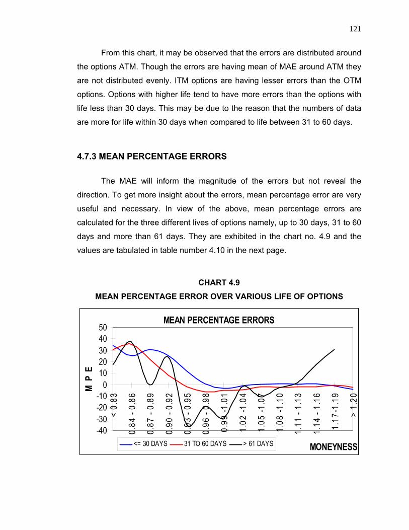
From this chart, it may be obs at the er distributed around

the options ing mean of MAE around ATM they

are not distributed evenly. ITM options

options. Options with higher life tend to e more errors than the options with

life less than 30 days. This may be due to

are more for life within 30 da

4.7.3 MEAN PERCENT ERR

The MAE will inform the magnitude of the errors but not reveal the

direction. To get more insight about the errors, mean percentage error are very

are

options namely, up to 30 days, 31 to 60

days and more than 61 days. They are exhibited in the chart no. 4.9 and the

values

MEAN PERCENTAGE ERROR OVER VARIOUS LIFE OF OPTIONS

erved th rors are

ATM. Though the errors are hav

are having lesser errors than the OTM

hav

the reason that the numbers of data

ys when compared to life between 31 to 60 days.

AGE ORS

useful and necessary. In view of the above, mean percentage errors

calculated for the three different lives of

are tabulated in table number 4.10 in the next page.

CHART 4.9

MEAN PERCENTAGE ERRORS

-40-30-20-10

01020304050

< 0.

83

0.84

86

0.87

89

0.90

92

0.93

95

0.96 0.99

0

1.02

0

1.05

07

1.08

10

1.11

13

1.14

16

1.1

19

> 1.

20

MONEYNESS

M P

E

- 0.

- 0.

- 0.

- 0.

- 0. -1

.

-1.

-1.

-1.

- 1.

- 1.

7-1.

98 1 4

<= 30 DAYS 31 TO 60 DAYS > 61 DAYS

122

TABLE 4.10

MEAN PERCENTAGE ERROR FOR VARIOUS LIFE OF OPTIONS I


MONEYNESS < = 30 DAYS

31- 60 DAYS

> 61 DAYS

< = 0.83 34.18 31.01 17.40 0.84 - 0.86 25.23 35.19 37.21 0.87 - 0.89 30.69 22.47 -0.08 0.90 - 0.92 25.44 8.21 24.09 0.93 - 0.95 11.81 -1.76 -34.84 0.96 - 0.98 0.77 -6.11 -19.08 0.99 -1.01 -2.97 -5.14 -29.09 1.02 -1.04 -1.05 -4.63 -1.45 1.05 -1.07 0.34 -1.80 -10.27 1.08 -1.10 0.95 -2.05 -2.48 1.11 - 1.13 0.40 -1.41 1.71 1.14 - 1.16 0.97 -1.83 17.76 1.17-1.19 -1.02 -0.71 30.85 > 1.20 -3.95 -1.97 NA

From the table and chart it may be observed that the mean percentage

errors vary for different lifes of options and has a definite pattern of decreasing

over increase in moneyness. As explained earlier, the data related to options

0 including for life more than 61 days can be omitted. After

omitting that the curves are smooth and show patterns, which is displayed in

chart no. 4.10.

less than 500

123

CHART 4.10

MEAN PERCENTAGE ERROR FOR DIFFERENT LIFE OF OPTIONS FOR DATA MORE THAN 5000

MEAN PERCENTAGE ERRORS

-8-6-4-202468

101214

M P

E

0.93 - 0.95 0.96 - 0.98 0.99 -1.0 .02 -1.04 1.05 -1.07 1.08 -1.10

MONEYNESS

1 1

<= 30 DAYS 31 TO 60 DAYS

From the curves exhibit ay erved redictability and

resultant errors are not only influenced by the lifes of options but also by the

moneyness.

So far the options were categorized into ee different types in the same

style of NSE. Now, in another angle, the options were categorized into eight,

each having te as d b he table no.4.11. During the

categorization it was observed that there exist small number of (18) outliers,

which distort the error pattern in a sign

using SAS and al me hes were id and taken off

from the sample. The calculated Mean percentage errors are tabulated in the

table no. 4.11.

ed, it m be obs that the p

thr

n days life detaile elow in t

ificant manner. Box-plots were drawn

by graphic thod t e outliers entified

124

TABLE 4.11

MEAN PERCENTAGE ERROR OVER VARIOUS LIVES OF OPTIONS II

LIFE IN DAYS

No. of data

Mean Absolute

Error

Mean Percentage

Error Percentage

of data Cumulative Percentage

of Data

0 - 10 20,160 0.16 3.35 21.01 21.01

11 - 20 23,635 0.19 3.52 24.64 45.65

21 - 30 31,062 0.20 -1.72 32.38 78.03

31 - 40 15,283 0.23 -1.70 15.93 93.96

41 - 50 4,480 0.26 -4.14 4.67 98.63

51 - 60 1,126 0.25 -8.43 1.17 99.80

61 - 70 133 0.22 -11.25 0.14 99.94

71 - 80 59 0.31 -17.34 0.06 100.00

The mean percentage errors vary from 3.35 to -17.34. If the mean

percentage errors for the data which are more than 5,000 at least are

considered reliable, then the errors are within 3.35 to -1.70 only. The table

enlightens us that the most of the traded options are having life within forty days

e sample, 93.96% of options got Mean percentage errors within

only. Out of th

3.35 to -1.70. If one includes the life within 41- 50 days, then the mean

percentage error slightly increases to - 4.14 but covers 98.63% of options of our

sample. To understand better, the same are furnished in the chart no. 4.11.

125

CHART 4.11

MEAN PERCENTAGE ERROR OVER VARIOUS LIFE OF OPTIONS


-

5.00

-20.00

15.00

LIFE IN DAYS

-10.00

-5.00

0.000 - 10 11- 20 21 - 30 31 - 40 41 - 50 51 - 60 61 - 70 71 - 80

EM

P

Though the mean percentage errors were very low, the mean

percentage errors were still show a patte m distribution.

The errors are positive for the op p to 20 day. The options having

more t

model over-prices the options within life of 20 days and under-prices the options

having life more than 20 days. The errors are stribut omly around

m stra p

be inferred that the biases exist with lifes of th s also

rn and not having rando

tions with life u

han 20 days have negative mean percentage errors. In other words, BS

not di

attern can be

e option

ed rand

observed. Ththe mean, but ore or less a ight line

the

us it can

.

126

4.8 BIASES OVE ATILIT F S RETU

the s e and strike price, a lained ter III,

luencing par r of the model is the volatility of stoc rns. M

over, i


The sample is observed for the actual volatility for all the twenty-eight

companies. The volatility varies from 0.16 to 0.95, with some meager data with

specific v ly

Dr.Reddys and Infosys. In view of the ab mple is categorized from

0.10 in steps of 0.10 till the volatility of 1.00 and volatilities 1.21 and 4. The

ratios. It can be observed that the figures related to less than 5000 are marked

R VOL IES O TOCK RNS

Next to tock pric s exp in chap the

more inf amete k retu ore

t is the only factor that is estimated in the model as other variables and

parameters are observable and taken directly. Hence, the study about volatility

is important and interesting. In the following sub chapters the analysis and the

findings are enumerated in detail.

olatility of 1.21 to 1.23 and 4.08 related to only two companies name

ove, the sa

categorization and the respective MAE are given in the table number 4.12. The

errors are given in rupees and rounded off to one rupee. MAE are expressed as

with shades and the figures may not represent the true value.

127

TABLE 4.12

L F S V S RETURNS

MEAN ABSO UTE ERRORS OR VARIOU OLATILITIE OF STOCK

Volatility No. of Data

Total Observed

Price Rs.

Total Absolute

Errors Rs.

Mean Absolute

Error

0.10-0.20 956 23,848 5,934 0.25

0.20-0.30 2 10,39, 1,80,263 0.1732,93 443

0.30-0.40 9 12,39,0 2,17,059 0.1830,18 08

0.40-0.50 6,35,6 1,20,958 0.1919,805 19

0.50-0.60 1,83,600 46,908 0.266,708

0.60-0.70 2,406 1,37,810 43,281 0.31

0.70-0.80 1,607 1,14,065 35,060 0.31

0.80-0.90 809 15,401 6,792 0.44

0.90-1.00 315 5,424 4,471 0.82

1.21-1.23 199 9,361 12,457 1.33

> 4 30 5,096 9,886 1.94 Rounded off to rupee

The MAE vary from 0.17 to 1.94. As usual, after omitting the options less

than 5,000, the errors systematically increases from 0.17 to 0.26 as the volatility

increases from 0.20 to 0.60. A pattern is observed as there exists a direct,

positive relation between the errors and the volatility of stock returns.

The errors seem to be low at low volatilities 0.20 - 0.30, 0.30-0.40, and

0.40-0.50. For the volatility is higher to 0.50, the errors increases at a faster rate

to 0.26. The pattern is much easily observed from the chart no. 4.12

128

CHART 4.12

MEAN ABSOLUTE ERROR FOR VARIOUS VOLATILITIES

MEAN A0.35

BSOLUTE ERROR FOR VOLATILITIES

0.30

0.00

0.05

0.10

0.15

0.20

0.25

0.20-0.30 0.30-0.40 0.40-0.50 0.50-0.60 0.60-0.70 0.70-0.80

VOLATILITY

M A

E

The errors are increasing with volatility and the model has prediction bias

over the volatility of stock returns. Some portion of these high errors may be

due the fact that the numbers of data are relatively low.

It is analyzed in another angle, for each category of moneyness, the

volatility is changed and the MAE are calculated, summarized and tabulated.

The MAE are then drawn in a chart and displayed in chart no. 4.13. The

influence of moneyness is seen as ITM options are having flat curves and

curves of OTM options tend to be steeper.

129

CHART 4.13

MEAN ABSOLUTE ERROR OVER VARIOUS VOLATILITY AND MONEYNESS

Mean Absolute Errors

0.58

0.080.30-0.40 0.40-0.50 0.50-0.60 0.60-0

0.18

.70

0.28

0.38

0.48

VOLATILITY

M A

E

0.90-0.92 0.93-0.95 0.96-0.98 0.99-1.01 1.02-1.04 1.05-1.07 1.08-1.10 1.11-1.13

130


As followed for other variables and parameters, mean percentage errors

re also calculated for different volatility, summarized and tabulated in table no.

.13. The volatility ranging from 0.20 to 0.50 contains 86.42 % of the data. It

cludes volatility of 0.50 - 0.60, 93.41% data are covered. The other

insignificant data were shown in shade. The plots of the mean percentage

errors are shown in chart no. 4.14

TABL 4.13

MEAN PERCENTAGE ERROR FOR VARIOUS VOLATILITY

a

4

in

E

Volatility No. of Data

Observed Option Price

Percentage Errors

0.10-0.20 956 23,848 28.68

0.20-0.30 32,932 039,443 13.24 1,

0.30-0.40 30,189 239,008 4.62 1,

0.40-0.50 19,805 635,619 -7.09

0.50-0.60 6,708 183,600 -20.93

0.60-0.70 2,406 137,810 -44.44

0.70-0.80 1,607 114,065 -32.77

0.80-0.90 809 15,401 -59.26

0.90-1.00 315 5,424 -114.51

1.21-1.23 199 9,361 -157.64

> 4 30 5,096 -206.79

131

CHART 4.14

DETAILS OF MEAN P RIOUS VOLATILITY ERCENTAGE ERROR FOR VA


-25

-20

-15

-10

-5

0

5

0.20-0.30 0.30-0.40 0.40-0.50 0.50-0.60VOLATILITY

M P

E

10

15

entage error is positive and high at 13.24 for the volatility

40 it drops to 4.62 and is negative

for the volatility range of 0.40 – 0.50 but magnitude-wise it increases to around

The mean perc

of 0.20 - 0.30. For next category of 0.30 – 0.

7. As volatility further increases, the mean percentage error raised to -20.93.

This high error may be due to the fact that the number of data is low at 6708

only for a period of 5 years and 10 months. A definite pattern of errors is

evidenced from the above chart. Thus, pricing biases do exist for volatility of

stock returns also.

132

4.9 R

ive. The model has biases over all the other

categorizes the option sample into

different RFR, analyses them and explains the findings in detail.

RISK – FREE INTEREST RATES I

ISK - FREE INTEREST RATE

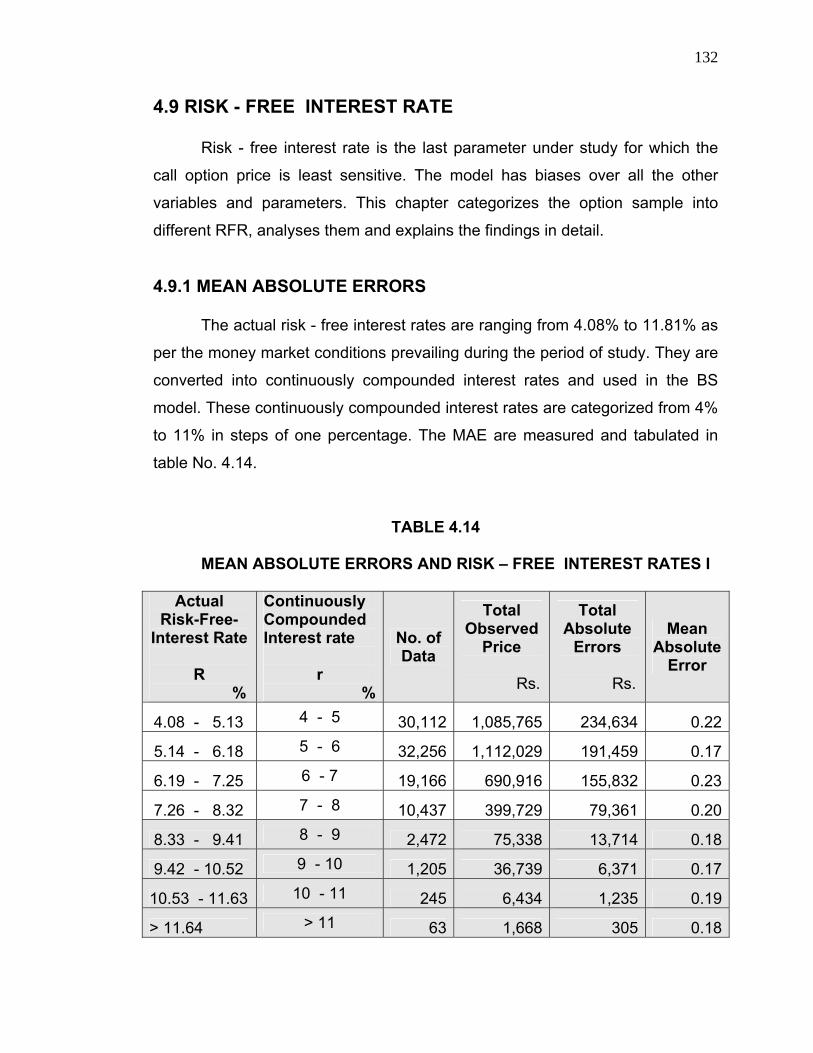
Risk - free interest rate is the last parameter under study for which the

call option price is least sensit

variables and parameters. This chapter


The actual risk - free interest rates are ranging from 4.08% to 11.81% as

per the money market conditions prevailing during the period of study. They are

converted into continuously compounded interest rates and used in the BS

model. These continuously compounded interest rates are categorized from 4%

to 11% in steps of one percentage. The MAE are measured and tabulated in

table No. 4.14.

TABLE 4.14

MEAN ABSOLUTE ERRORS AND

Actual Risk-Free-

Interest Rate

R %

Continuously Compounded Interest rate

r %

No. of Data

Total Observed

Price

Rs.

Total Absolute

Errors

Rs.

Mean Absolute

Error

4.08 - 5.13 4 - 5 30,112 1,085,765 234,634 0.22

5.14 - 6.18 5 - 6 32,256 1,112,029 191,459 0.17

6.19 - 7.25 6 - 7 19,166 690,916 155,832 0.23

7.26 - 8.32 7 - 8 10,437 399,729 79,361 0.20

8.33 - 9.41 8 - 9 2,472 75,338 13,714 0.18

9.42 - 10.52 9 - 10 1,205 36,739 6,371 0.17

10.53 - 11.63 10 - 11 245 6,434 1,235 0.19

> 11.64 > 11 63 1,668 305 0.18

133

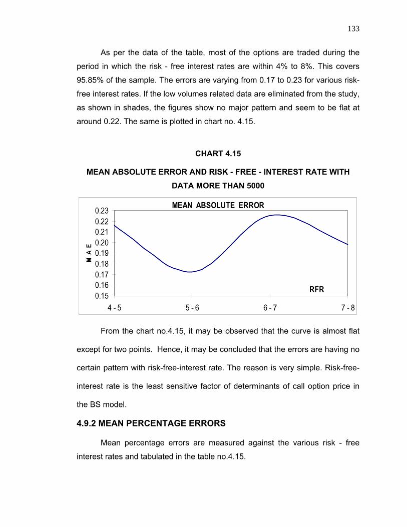
As per the data of the table, most of the options are traded during the

period in which the risk - free interest rates are within 4% to 8%. This covers

95.85%

how no major pattern and seem to be flat at

around

CHART 4.15

MEAN ABSOLUTE ERROR AND RISK - FREE - INTEREST RATE WITH DATA MORE THAN 5000

of the sample. The errors are varying from 0.17 to 0.23 for various risk-

free interest rates. If the low volumes related data are eliminated from the study,

as shown in shades, the figures s

0.22. The same is plotted in chart no. 4.15.

MEAN ABSOLUTE ERROR

0.150.160.170.180.19

20

4 - 5 5 - 6 6 - 7 7 - 8

RFR

M A

0.0.210.220.23

E

From the chart no.4.15, it may be observed that the curve is almost flat

except for two points. Hence, it may be concluded that the errors are having no

certain pattern with risk-free-intere reason is very simple. Risk-free-

interest rate is ption price in

the BS model.


Mean percentage errors are measured against the various risk - free

interest rates and tabulated in the table no.4.15.

st rate. The

the least sensitive factor of determinants of call o

134

TABLE 4.15

MEAN PERCENTAGE ERROR AND RISK - FREE - INTEREST RATE II

Actual Risk - Free - Interest Rate

R

%

Continuously Compounded Interest rate

r

%

No. of Data

Total

Observed Price

Rs.

Mean

Percentage Error

Rs.

4.08 - 5.13 4 - 5 30,112 1,085,765 -1.45

5.14 - 6.18 5 - 6 32,256 1,112,029 5.26

6.19 - 7.25 6 - 7 19,166 690,916 -5.71

7.26 - 8.32 7 - 8 10,437 399,729 1.89

8.33 - 9.41 8 - 9 2,472 75,338 7.00

- 10.52 9.42 9 - 10 1,205 36,739 -7.94

10.53 - 11.63 10 - 11 245 6,434 -8.66

> 11.64 > 11 63 1,668 -0.87

CHART 4.16

MEAN PERCENTAGE ERROR AND RISK - FREE - INTEREST RATE


2

4

6

-8

-6

-4

-2

04 - 5 5 - 6 6 - 7 7 - 8

RFR

M P

E

135

From the above table and chart, it may be inferred that the mean

uted against the risk – free interest rate and

no definite pattern is available. Hence, there is no bias on the model. This is

coincid

individual absolute errors is anal of the options it is less than or

equal to Rs.1.27, the next 25% options got it in between Rs.1.27 to Rs.3.12.

The n of the options have

it less than Rs. 15.62 and greater than Rs. 7.03. When compared to the

observed call option price as high as Rs.1200 and above, these errors may not

be high. The Mean percentage errors vary from -3.51 to 7.10 depending upon

the moneyness. That is the BS model predicts the call option price with a

minimum accuracy of 92.90% and a maximum of 96.49%; mean 95.4%.

Howe side than

the low 84.42%;

the n 9%. The

predic od. The

research paper of Bakshi, Gurdip, Cao, Charles, and Chen, Zhiwu [10],

“Empirical Performance of Alternative Option pricing Models” where, 38,749 call

options (S&P 500) for a period of June 1988 to May 1991, the Mean percentage

pricing

ictability varies from 34.22% to 97.51%. Fortune, Peter

[53], in his findings inferred that the errors vary from 10 to 100%. It may be

percentage error is randomly distrib

ing with the findings of MAE above.

4.10 CONCLUSION

The predictability of the model is checked by mainly measuring MAE and

mean percentage errors. The median-based percentiles also calculated. As far

as the MAE are concerned, it varied from 0.12 to 0.43 for the moneyness of

1.10 to 0.93. The average is 0.24. That is according to the MAE predictability of

the model vary from 57% to 88%; mean being 76%. When the distribution of

yzed, for 25%

ext 25% have it in between Rs. 3.12 to Rs. 7.03; 15%

ver, the predictability of most of the options is biased on higher

er side. Middle 50% of options are having the predictability of

ext 30% of options are having the predictability of 76.2

tability of the model in Indian Option Market is extremely go

errors vary from 2.49% to -65.78% for the moneyness range of 1.06 to

0.94. That is, the pred

136

concluded that the model’s predictability in Indian Option Market is comparably

better than the predictability of the model in overseas option markets as per the

above research papers published abroad.

ther as

oneyness and all the others are individually tested. The MAE and mean

percen

or of the model.

Merville [94], Bakshi, Gurdip [10], and Rubinston [118] also

confirmed the existence of the biases. But the biases are not in the same

direction in all the above cases. In Indian market, the model systematically

underpriced deep OTM options and the deep ITM options. The near OTM

options and ATM options are overpriced. This is against the prediction of Black,

Fisher

reverse of the

biases reported by Fisher Black [23].

e used to rectify the errors

also. For example, if the model under-prices the options of moneyness 1.02 -

1.04 by 4.50%; the investor can adjust

error. Thu

correct pr rd of caution is that the systematic

biases may change over different periods of observation like, recession period

All the variables and parameters of the model are studied towards

prediction biases, if any. The stock price and strike price are used toge

m

tage errors are showing definite biases over change in moneyness,

volatility and life of the options. The model does not exhibit any bias over risk -

free - interest rate, which is the least sensitive fact

Our findings are in line with the biases that are explained in the papers of

Geske, Robert and Roll, Richard in their paper [55], “The Black –Scholes call

option pricing model is subject to systematic empirical biases. These biases

have been documented with respect to the option’s exercise price, its time to

expiration, and the underlying common stock’s volatility…”. Black, Fisher [23],

MacBeth and

[23] that the model systematically underpriced deep OTM options and

overprices the deep ITM options. MacBeth and Merville [94] confirmed by the

strike biases for the period 1975-1976, but found that it was the

But, these biases are systematic and can b

the price accordingly and correct the

s as far as the biases are systematic it can be used to predict the

ice by adjustments. However, a wo

137

or boo

be use

m period. Hence, the biases have to be determined periodically and can

d effectively.

CHAPTER IV PREDICTABILITY OF THE BS MODEL IN INDIAN

Documents

Transcript of CHAPTER IV PREDICTABILITY OF THE BS MODEL IN INDIAN