CHAPTER-I

INTRODUCTION AND REVIEW OF SPLINE FUNCTION

APPROXIMATIONS

1.1 Introduction

The mathematical formulation of a physical process requires background in

related field and mathematical tools. The formulation results in mathematical

statements, mostly differential equations, relating quantities of interest in the design of

physical process. In a numerical simulation of a physical process we employ some

numerical methods and computing facility. Most engineers, scientists and applied

mathematicians studying physical phenomena are involved with two major tasks:

I: Mathematical formulation of physical processes

II: Numerical analysis of the mathematical model

The numerical methods developed may broadly be classified into the following

three types:

(i) Finite difference methods

(ii) Finite element and Wavelet methods

(iii) Spline function approximation methods

The thesis is concerned with the development of polynomial and non-

polynomial spline fimction approximation methods to obtain numerical solutions of

ordinary and partial differential equations have been investigated. The use of spline

functions dates back at least to the beginning of previous century. Piecewise linear

fimctions had been used in connection with the Peano's existence proof for the solution

to the initial value problems of the ordinary differential equations, although these

functions were not called splines. Splines were first identified in the work of

Schoenberg, Sard and others. Usually a spline is a piecewise polynomial function

defined in a region D, i.e, a function for which there exist a decomposition of D into

subregions in each of which the function is a polynomial of some degree m. Also the

function, as a rule, is continuous in D, together with its derivatives of order upto (m-1)

(Marchuk [80]). In other words spline function is a piecewise polynomial satisfying

certain conditions of continuity of the fiinction and its derivatives. The applications of

spline as approximating, interpolating and curve fitting functions have been very

successful (Ahlberg at al [2], Greville [48], Prenter [92], Micula [82]). It is also

interesting to note that the cubic spline is a close mathematical approximation to the

draughtsman's spline, which is a widely used manual curve-drawing tool. It has been

shown by Schoenberg [107] that a curve drawn by a mechanical spline to a first order of

approximation is a cubic spline function. Further, the solution of a variety of problems

of 'best approximation' are the spline function approximations. Later on spline

functions recieved a considerable amount of attention in both theoretical and practical

studies.

A number of authors have attempted polynomial and non-polynomial spline

a^oximation methods for the solution of differential equations; De Boor [32-34],

Ahlberg et al [2], Loscalzo and Talbot [77-78], Bickley [15], Fyfe [44,46], Albasiny

and Hoskins [3], Sakai [103-105 ], Russell and Shampine [102], Micula [81,82], Rubin

and Khosla [101], Rubin and Graves [100],Daniel and Swartz [30],Archer [7], Patricio

[90-91], Tewarson [116-117], Usmani et al [122,124-125], Jain and Aziz [55-57], Surla

et al [111-114], Iyengar and Jain [53], Chawla and Subramanian [18-20], Irodotou-

EUina and Houstis [52], Rashidinia [93], Fairweather and Meade [40] and others.

Spline functions of maximum smoothness were first considered in the numerical

solution of initial value problems in ordinary differential equations by Loscalzo and

Talbot [77-78] and many interesting connections with standard numerical integration

techniques have been established. For example, the trapezoidal rule and the Milne-

Simpson predictor- corrector method fall out as special cases of such spline

approximations. The main reason why the above mentioned applications of spline

functions to the numerical integration of ordinary differential equations leads to

unstable methods is because the resulting numerical approximations are, in a certain

sense too smooth (Varga [126]). Loscalzo and Schoenberg [76] have shown that the

use of Hermite-Splines of lower order smoothness avoids completely the problem of

unstability. The spline functions have been used by a number of authors to solve both

initial and boundary value problems of ordinary and partial differential equations. The

use of cubic splines for the solution of linear two point boundary value problems was

suggested by Bickley [15]. His main idea was to use the 'condition of continuity' as a

discretization equation for the linear two point boundary value problems. Later, Fyfe

[44] discussed the application of deferred corrections to the method suggested by

Bickley by considering again the case of (regular) linear boundary-value problems.

However, it is well known since then that the cubic spline method of Bickley

gives only O(h^) convergent approximations. But cubic spline itself is a fourth-order

process [92]. It is therefore natural to look for an alternative method which would give

fourth order approximations using cubic splines. We also find that the application of

the spline function to the solution of convection-diffusion problems has not been very

encouraging. To be able to deal effectively with such problems we introduce spline

functions containing a parameter co. These are non-polynomial splines defined through

the solution of a differential equation in each subinterval. The arbitrary constants being

chosen to satisfy certain smoothness conditions at the joints. These splines belong to

the class C and reduce into polynomial splines as parameter (o-> 0. The exact form of

the spline depends upon the maimer in which the parameter is introduced. We have

studied parametric spline function, spline imder compression, spline under tension and

adaptive spline. A number of spline relations have been obtained for subsequent use. A

wide class of singular boundary value problems have also been successfully solved

.The sextic spline function has been applied to the vibrating beam equation.

The singular perturbation mathematical model plays an important role in

modelling fluid processes arising in applied mechanics. We have either the stiff system

of initial boundary value problems or the convection-diffusion problems. It has been

realized that when conventional methods are applied to obtain numerical solution, the

step size must be limited to small values. Any attempt to use a larger step size results in

the calculations becoming imstable and producing completely erroneous results. In

recent years, considerable attention has been devoted to the formulation and

implementation of, in essence, modified spline methods for the solution of certain

classes of elliptic boimdary value problems on rectangles, see for example Houstis et al

[51]. It is interesting to note that this approach was adopted by Irodotou-EUina and

Houstis [52],in their quintic spline collocation methods for general linear fourth order

two point boundary value problems. Another quintic spline method requiring a uniform

mesh for a non-linear fourth order boundary value problem is due to Chawla and

Subramanian [20]. This method is based on Bickley's idea [15] of using the continuity

condition to construct a cubic spline approximation, but here it is used only after some

other method (e.g., a finite difference method) has been used to obtain accurate nodal

values. Fairweather and Meade [40] provide a comprehensive survey of both

orthogonal and modified spline collocation methods for solving ordinary and partial

differential equations.

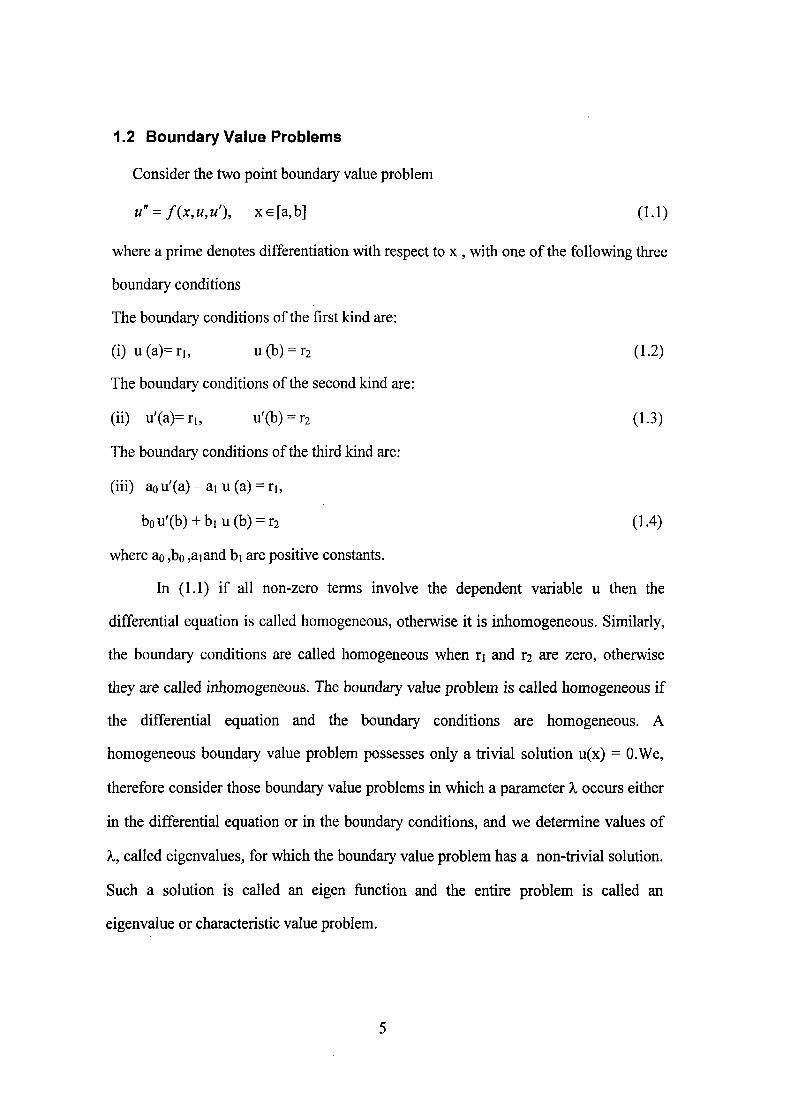
1.2 Boundary Value Problems

Consider the two point boundary value problem

u" = f(x,u,u'), x€[a,b] (1.1)

where a prime denotes differentiation with respect to x , with one of the following three

boundary conditions

The boundary conditions of the first kind are:

( i)u(a)=r, , u(b) = r2 (1.2)

The boundary conditions of the second kind are:

(ii) u'(a)=ri, u'(b) = r2 (1.3)

The boundary conditions of the third kind are:

(iii) aou'(a)-aiu(a) = ri,

bou'(b) + biu(b) = r2 (1.4)

where ao ,bo ,aiand bi are positive constants.

In (1.1) if all non-zero terms involve the dependent variable u then the

differential equation is called homogeneous, otherwise it is inhomogeneous. Similarly,

the boundary conditions are called homogeneous when ri and r2 are zero, otherwise

they are called inhomogeneous. The boundary value problem is called homogeneous if

the differential equation and the boundary conditions are homogeneous. A

homogeneous boundary value problem possesses only a trivial solution u(x) = O.We,

therefore consider those boundary value problems in which a parameter X occurs either

in the differential equation or in the boundary conditions, and we determine values of

X, called eigenvalues, for which the boundary value problem has a non-trivial solution.

Such a solution is called an eigen function and the entire problem is called an

eigenvalue or characteristic value problem.

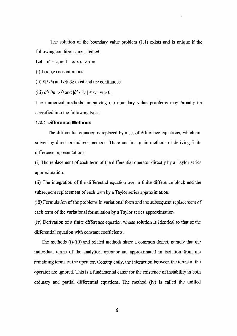
The solution of the boundary value problem (1.1) exists and is unique if the

following conditions are satisfied:

Let u' = z, and - oo < u, z < oo

(i) f (x,u,z) is continuous,

(ii) 5f/ dn and df/ dz exist and are continuous,

(iii) 5f/ au > 0 and |5f / 5z I < w, w > 0 .

The numerical methods for solving the boundary value problems may broadly be

classified into the following types:

1.2.1 Difference Methods

The differential equation is replaced by a set of difference equations, which are

solved by direct or indirect methods. There are four main methods of deriving finite

difference representations.

(i) The replacement of each term of the differential operator directly by a Taylor series

approximation.

(ii) The integration of the differential equation over a finite difference block and the

subsequent replacement of each term by a Taylor series approximation,

(iii) Formulation of the problems in variational form and the subsequent replacement of

each term of the variational formulation by a Taylor series approximation,

(iv) Derivation of a finite difference equation whose solution is identical to that of the

differential equation with constant coefficients.

The methods (i)-(iii) and related methods share a common defect, namely that the

individual terms of the analytical operator are approximated in isolation fi:om the

remaining terms of the operator. Consequently, the interaction between the terms of the

operator are ignored. This is a fundamental cause for the existence of instability in both

ordinary and partial differential equations. The method (iv) is called the unified

difference representation. Clearly, in this case the term interactions are included, and

no possibility of instability can exist.

1.2.2 Shooting Method

These are initial value problem methods. This method requires good initial

guesses for the slope and can be applied to both linear and non-linear problems. Its

main advantage is that it is easy to apply. The main steps involved in this method are

(i) Transformation of the boundary value problem into an initial value problem.

(ii) Solution of the initial value problem by Taylor's series method, or Runge-Kutta

method, etc.

In practice, the shooting method is quite slow. Therefore we ordinarily use finite

difference and spline methods for solving boundary value problems.

1.2.3 Finite Element Method

The finite element method was introduced as a variationally based technique of

solving differential equations. A continuous problem described by a differential

equation is put into an equivalent variational form, and the approximate solution is

assumed to be a linear combination, 2]*';^y' °^ approximation functions ^j. The

parameters Cj are determined using the associated variational form. The finite element

method provides a systematic technique for deriving the approximation fimctions for

simple sub-regions by which a geometrically complex region can be represented.

In the finite element method, in general we seek an approximate solution u to a

differential equation in the form

n m

7=1 j=\

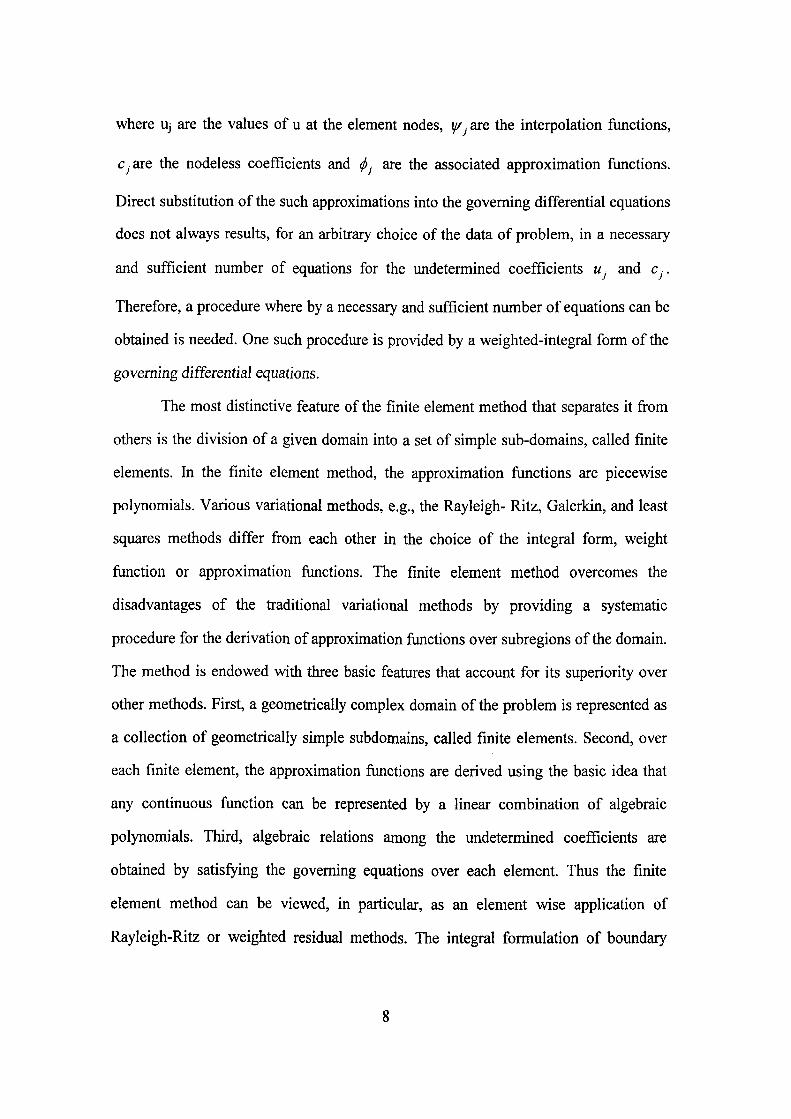
where Uj are the values of u at the element nodes, y/j are the interpolation functions,

c^are the nodeless coefficients and (fij are the associated approximation functions.

Direct substitution of the such approximations into the governing differential equations

does not always results, for an arbitrary choice of the data of problem, in a necessary

and sufficient number of equations for the undetermined coefficients Uj and Cj.

Therefore, a procedure where by a necessary and sufficient number of equations can be

obtained is needed. One such procedure is provided by a weighted-integral form of the

governing differential equations.

The most distinctive feature of the finite element method that separates it from

others is the division of a given domain into a set of simple sub-domains, called finite

elements. In the finite element method, the approximation functions are piecewise

polynomials. Various variational methods, e.g., the Rayleigh- Ritz, Galerkin, and least

squares methods differ from each other in the choice of the integral form, weight

function or approximation functions. The finite element method overcomes the

disadvantages of the traditional variational methods by providing a systematic

procedure for the derivation of approximation functions over subregions of the domain.

The method is endowed with three basic features that account for its superiority over

other methods. First, a geometrically complex domain of the problem is represented as

a collection of geometrically simple subdomains, called finite elements. Second, over

each finite element, the approximation functions are derived using the basic idea that

any continuous function can be represented by a linear combination of algebraic

polynomials. Third, algebraic relations among the undetermined coefficients are

obtained by satisfying the governing equations over each element. Thus the finite

element method can be viewed, in particular, as an element wise application of

Rayleigh-Ritz or weighted residual methods. The integral formulation of boundary

value problems comes from the fact that variational methods of approximation are

based on the weighted integral statements of governing equations. Since, the finite

element method is a technique for constructing approximation functions required in an

element wise application of any variational method, it is necessary to study the

weighted integral formulation and the weak formulation of differential equations. In

addition, weak formulation also facilitates, in a natural way the classification of

boundary conditions into natural and essential boundary conditions, which play a

crucial role in derivation of the approximation fimctions and selection of nodal degrees

of the freedom of finite element model.

1.2.4 Wavelet Method

Another important method for the numerical solution of ordinary and partial

differential equations is Wavelet method. Wavelet theory is an extension of Fourier

theory (See Amaratunga et al [6], Beylkin et al [14], Chui [22]).

In Multi-Resolution analysis, orthonormal bases of L2(R) are constructed as follows;

Let (j)e L2(R) and we define (|)j k, j ,keZ as follows

(t)j,k(x) = 2J'2^(2Jx-k)

Let Vj = closure [())j,k; keZ] for all jeZ be a family of subspaces of L2(R) such that

VjC Vj+i for all j eZ and closure (Ujez Vj) = L2(R).

For each j eZ, we define the space Wj such that Vj+i= Vj © Wj

Now we define

\j;j,k(x) = 2^'^ \\i (2 x-k), keZ and the space Wj define by

Wj == closure [ij/jjc; keZ] is generated by \\) and hence L2(R) = © jez Wj.

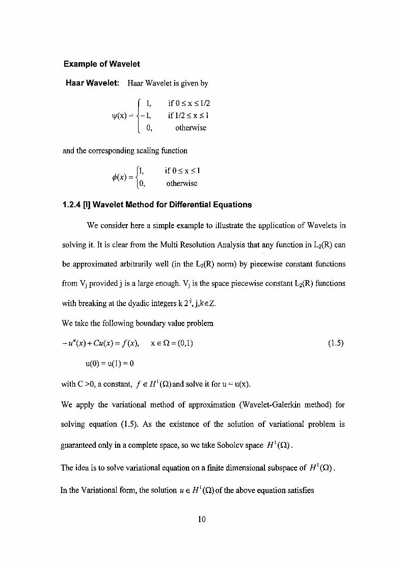
Example of Wavelet

Haar Wavelet: Haar Wavelet is given by

V)/(X)

1, i f 0 < x < l / 2 •1, i f l / 2 < x < l 0, otherwise

and the corresponding scahng function

fl, i f O < x < l

[0, otherwise

1.2.4 [I] Wavelet Method for Differential Equations

We consider here a simple example to illustrate the application of Wavelets in

solving it. It is clear from the Multi Resolution Analysis that any function in L2(R) can

be approximated arbitrarily well (in the LiCR) norm) by piecewise constant functions

from Vj provided j is a large enough. Vj is the space piecewise constant L2(R) functions

with breaking at the dyadic integers k 2"\ j ,keZ.

We take the following boundary value problem

-u''(x) + Cuix) = f(x), xeQ- (0 , l ) (1.5)

u(0) = u(l) = 0

with C >0, a constant, f & H^ (Q) and solve it for u = u(x).

We apply the variational method of approximation (Wavelet-Galerkin method) for

solving equation (1.5). As the existence of the solution of variational problem is

guaranteed only in a complete space, so we take Sobolev space / / ' (Q).

The idea is to solve variational equation on a finite dimensional subspace of i / ' (Q).

In the Variational form, the solution u e ^ ' ( Q ) of the above equation satisfies

10

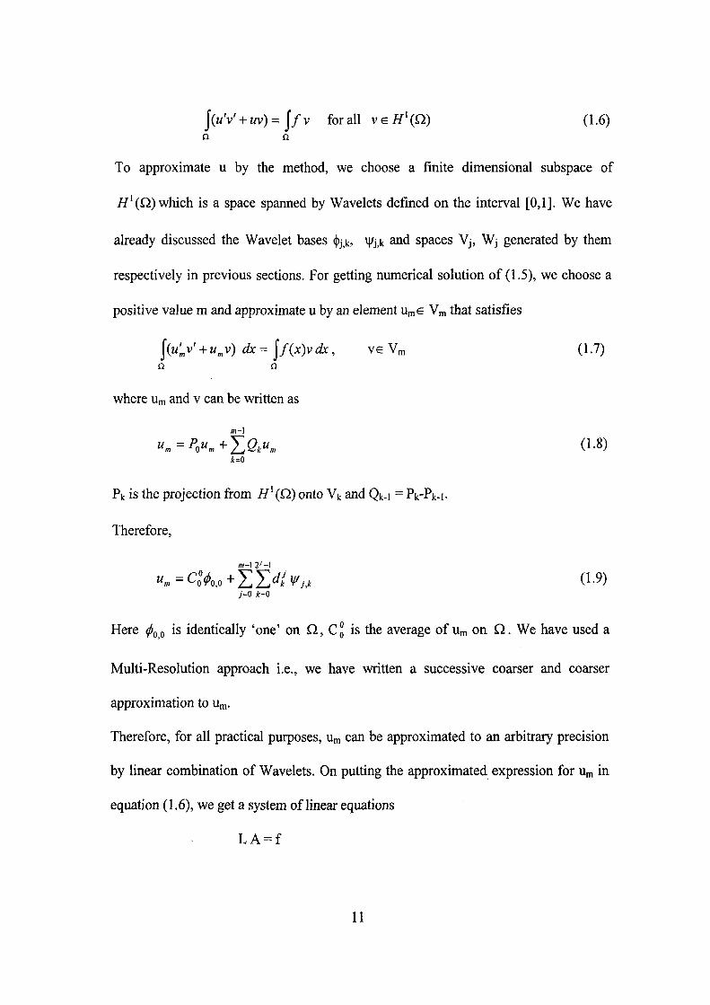
J(MV + WV)=J /V for all ve/ / ' (Q) (1.6) n n

To approximate u by the method, we choose a finite dimensional subspace of

/ / ' (Q) which is a space spanned by Wavelets defined on the interval [0,1]. We have

already discussed the Wavelet bases (t)j,k, Vj.k and spaces Vj, Wj generated by them

respectively in previous sections. For getting numerical solution of (1.5), we choose a

positive value m and approximate u by an element Ume Vm that satisfies

{(">' +".V) dx=lf(x)vdx, V6 Vn, (1 .7)

Q n

where Um and v can be written as

m-l

*:=0

Pk is the projection fi-om H\Q) onto Vk and Qk-i == Pk-Pk-i-

Therefore,

m-l 2^-1

7=0 *:=0

Here ^QQ is identically 'one' on Q, C^ is the average of Um on Q. We have used a

Multi-Resolution approach i.e., we have written a successive coarser and coarser

approximation to Um.

Therefore, for all practical purposes, Um can be approximated to an arbitrary precision

by linear combination of Wavelets. On putting the approximated expression for Um in

equation (1.6), we get a system of linear equations

L A - f

11

which can be solved using suitable methods.

1.3 Solution of Tridiagonal System

Consider the system of equations Au = b

where

-r ,

•Pi

1

-Pi Qi -h

0 -Pn 9N

A special case of tridiagonal system of equations arises in the numerical solution of the

differential equations. The tridiagonal system is of the form

-/'^V,+^«"«-^«««.i =^«. 1<«<A^ (1.10)

where pi, rn are given and UQ, Un+i are known form the boundary conditions of the

given problem. Assume that

;7„>0,qn>0, rn>0 and q„ >p„+r„ (1.11)

for 1 < « < A ( that is A is diagonally dominant). However, this requirement is a

sufficient condition. For the solution of (1.10) consider the difference relation

w„ =anUn+i+Pn, 0<n<N.

From (1.12) we have

Un.l=an-lUn+pn-l

Eliminating Un-i from (1.10) and (1.13), we get

(1.12)

(1.13)

w . = (ln-P.a„.\

-w«+i + d„+pj„-^n-Pn«n-

(1.14)

12

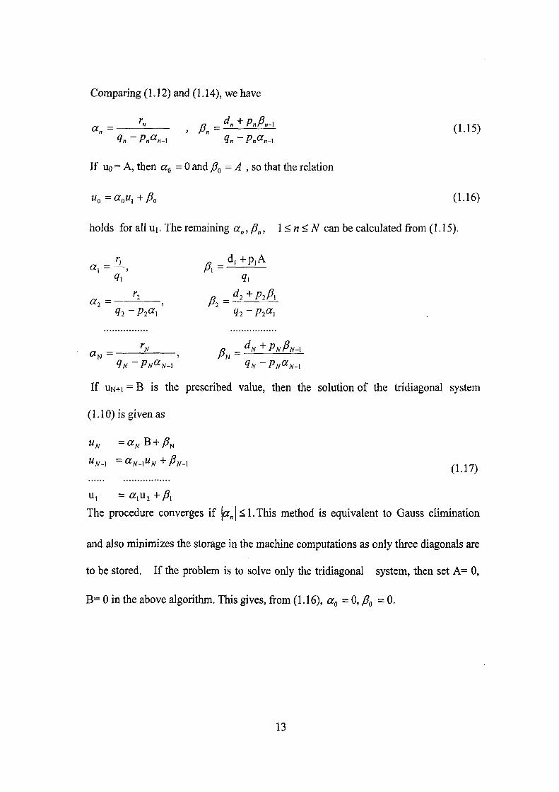
Comparing (1.12) and (1.14), we have

«„= '- , P„J"^P"^"-' (1.15)

If uo = A, then «(, = 0 and yo = ^ , so that the relation

"o=«o"i+y^o (1-16)

holds for all ui. The remaining a„,p„, \<n<N can be calculated from (1.15).

?i q

CCj — 5 Pi ~

1N-PN(^N-\ ^N-P^f^N-X

If UN+1 = B is the prescribed value, then the solution of the tridiagonal system

(1.10) is given as

(1.17)

u, = a,U2 +y9,

The procedure converges if |a„|<l.This method is equivalent to Gauss elimination

and also minimizes the storage in the machine computations as only three diagonals are

to be stored. If the problem is to solve only the tridiagonal system, then set A= 0,

B= 0 in the above algorithm. This gives, Jfrom (1.16), org = 0, / g = 0.

13

1.4 Solution of Pentadiagonal System

We can easily extend the method of solution of a tridiagonal system to a five band

system by writing the system of equations obtained in the solution of the differential

equation

w^"'+/(x)M = g(x), f(x)>0, xe[a,b] (1.18)

subject to the boundary conditions

u(a) = ai, u"(a) = Pi

u(b) = a2, u"(b) = |i2 (1.19)

(see p.220 [54]) as follows

C, D,

B, C- D. A j B j C j D3 E3

'•N-l B N-l

0

'N-l D

B.

u,

• A ' - I

\"N J

a.

a N-l

y^N J (1.20)

where Ai, Bj ,Ci, Dj, Ej, and a] are the known quantities. As in section (1.3) we assume

the following recurrence relations

u =h -0) u .-y u _, 0<n<N n n n n + \ ' n n + 2

(1.21)

We use (1.21) to find Un-i and Un.2 and substitute them in the equation

A„u„., +B„u„, +C„u„ +D„u„„ +E„u„,3 =«: , 2 <n<N-2 (1.22)

and by comparing it with (1.21), we get

14

h =(a'„-A h ^-S h .)/co*

a =(D„ -5 Y ^)lco* n " n'n-V " (1.23)

where S„ =B„-A„co„,^

In view of the first boundary conditions in (1.19) we have

ho =uo, ©0=0, Yo=0 (1.24)

Equation (1.21) will be identical with the first equation in (1.20) if

h^ = a\ Ico\, co^ = D, /co', /, - £, /cy' (1.25)

where <W|' = ci.

The second condition in (1.19) will be fulfilled if

UN = 0

The relation (1.23) together with (1.24) and (1.25) will hold for 0 < n < N if UN-I = 0

and hence u,^ = h^ -a)„u^^^

The values UN-I, UN-2, , U2, ui can be obtained by backward substitution in the equation

^n=K -^«"«.i -r„w«.2' n ^ N - 1 , 2,1.

1.5 Spline Functions

A spline" fimction is generally regarded as a piecewise polynomial satisfying

certain conditions of continuity of the fimction and its derivatives. The idea has been

extended in various directions. The applications of the splines as approximating,

interpolating and curve fitting fimctions have been very successful (Ahlberg et al [2],

Greville [48], Prenter [92]). It has been shown by Schoenberg [107] that a curve drawn

by a mechanical spline to a first order of approximation is a cubic spline fimction.

15

Further, the solution of a variety of problems of 'best'approximation are the spHne

function approximations.

We consider a mesh A with nodal points Xj on [a, b] such that

A:a = xo < xi < X2 < XN-I<XN= b where /?. =Xj-Xj_^ , for j=l(l)N. Assume

we are given the values \iij j of a function u(x) , with [a ,b] as its domain of

definition. A spline function of degree m with nodes at the points Xj, j =0,1,2...N is a

function SA(X) with the following properties:

(a) In each sub interval [xj,Xj+i ], j =0,1,...N-1, SA(X) is a polynomial of degree m.

(b) SA(X) and its first (m-1) derivatives are continuous on [ a,b]. If the function SA(X)

has only (m-k) continuous derivatives, then k is defined as the deficiency of the

polynomial spline and is usually denoted by SA(m,k), see [101]. The cubic spline is a

piecewise cubic polynomial of deficiency one, e.g. SA(3,1). The cubic spline procedure

can be described as follows

Consider a function u(x) such that at the mesh points Xi ,u(xi)= Uj . A cubic

polynomial is specified on the interval [xj.i, Xj] . The four constants are related to the

function values Uj.i,Uj as well as certain spline derivatives mj.i,mj or Mj.i, Mj .The

quantities mj ,Mj are the spline derivative approximations to the function derivatives

u'(Xj), u''(Xj) respectively. Similarly considered on the interval [x j,Xj+i] . The

continuity of the derivatives is then specified at Xj. The procedure results in equations

for mj, Mj, j = 1,2, ....N-1. Boundary conditions are required at j =0 and j = N. The

system is closed by the governing differential equation for u(xj), where the derivatives

are replaced by their spline approximations mj ,Mj.

The spline functions approximation has the following advantages:

16

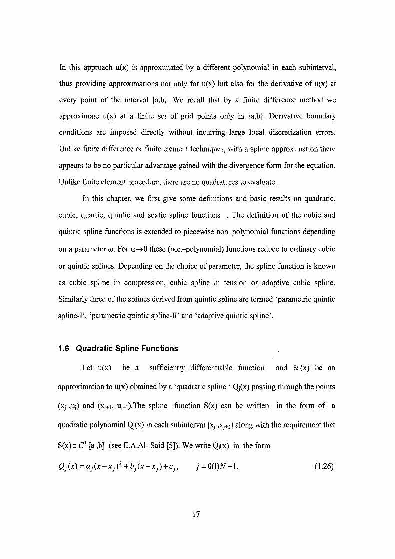
In this approach u(x) is approximated by a different polynomial in each subinterval,

thus providing approximations not only for u(x) but also for the derivative of u(x) at

every point of the interval [a,b]. We recall that by a finite difference method we

approximate u(x) at a finite set of grid points only in [a,b]. Derivative boundary

conditions are imposed directly without incurring large local discretization errors.

Unlike finite difference or finite element techniques, with a spline approximation there

appears to be no particular advantage gained with the divergence form for the equation.

Unlike finite element procedure, there are no quadratures to evaluate.

In this, chapter, we first give some definitions and basic results on quadratic,

cubic, quartic, quintic and sextic spline functions . The definition of the cubic and

quintic spline ftinctions is extended to piecewise non-polynomial functions depending

on a parameter co. For co^O these (non-polynomial) functions reduce to ordinary cubic

or quintic splines. Depending on the choice of parameter, the spline fiinction is known

as cubic spline in compression, cubic spline in tension or adaptive cubic spline.

Similarly three of the splines derived from quintic spline are termed 'parametric quintic

spline-F, 'parametric quintic spline-IF and 'adaptive quintic spline'.

1.6 Quadratic Spline Functions

Let u(x) be a sufficiently differentiable function and M(X) be an

approximation to u(x) obtained by a 'quadratic spline ' Qj(x) passing through the points

(xj ,Uj) and (xj+i, Uj+i).The spline fimction S(x) can be written in the form of a

quadratic polynomial Qj(x) in each subinterval [xj ,Xj+i] along with the requirement that

S(x)e C' [a ,b] (see E.A.Al- Said [5]). We write Qj(x) in the form

Qj(x) = ajix-Xjy+bj{x-Xj) + Cj, j = Q{l)N-\. (1.26)

17

The set of quadratic polynomials, using a possibly different polynomial in each

subinterval defines a smooth approximation to u(x) .We further require that the values

of first order derivative be the same for the pair of quadratics that join at each grid

point Xj. We determine the three coefficients in (1.26) in terms of

M . ,/2 ,mj and Mj^,/2, where

(//) Q ; ( X P - m^

we obtain the following relations via a straightforward calculation

^j = ^^7+1/2 (1.27)

h /2^ <^j = ^i.m -^^j - y M^^,/2, j - 0(1)N -1 . ^ ^ ^ ^ j . ^ ^ ^^^ continuity

of quadratic spline and its first derivative at the grid points Xj where the two

quadratics Qj-i(x) and Qj(x) join, we have

Q'/_Uxj)= Qf\xj), / . = 0,1. (1.28)

Using (1.26), (1.27) and (1.28), we get the following relations

/2(m^ +mj,) = 2(u.,„, -uj_,^,)-jh' (M^,,,, +3Mj_,^,) (1.29)

/z(mj-m^,)=h^Mj,/, (1.30)

which yield

1 2 ^nij = (Uj,,/2 -Uj_y,)--h (Mj„/2 -Mj.y^y (1.31)

The elimination of mi fi-om (1.29) and (1.31) gives the following recurrence relation

18

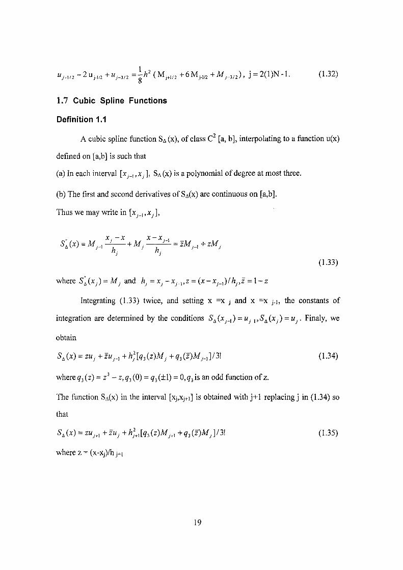
";.,/2-2u^,,2+V3/2 =^^ ' (M, ,„ ,+6Mj , / ,+M,_3 , , ) , j = 2(l)N-l . (1.32)

1.7 Cubic Spline Functions

Definition 1.1

A cubic spline function SA(X), of class C [a, b], interpolating to a function u(x)

defined on [a,b] is such that

(a) In each interval [x^_, ,Xj], SA (X) is a polynomial of degree at most three.

(b) The first and second derivatives of SA(X) are continuous on [a,b].

Thus we may write in [x^_, ,x^ ],

S: (x) - M, , ^ ^ + M, ^^"' = zM, , + zM,

(1.33)

where 5^(x^) = M^ and /z =x^-x^_,,z = (x-x^_,)/ft^.,z = l - z

Integrating (1.33) twice, and setting x =x j and x =x j.i, the constants of

integration are determined by the conditions S^ (x^_|) = M _, , S^ (Xj ) = Uj. Finaly, we

obtain

S, (X) = zu^ + zu^_, + h^ [q, iz)Mj + q, {z)M,_, ] / 3! (1.34)

where j (z) = z - z, 3 (0) = ^3 (± 1) = 0, 3 is an odd function of z.

The function SA(X) in the interval [Xj,Xj+i] is obtained with j+1 replacing] in (1.34) so

that

5,(x) = zu,„ +zuj +hl,[q,{z)Mj,, +^3(z)MJ/3! (1.35)

where z = (x-Xj)/hj+i

19

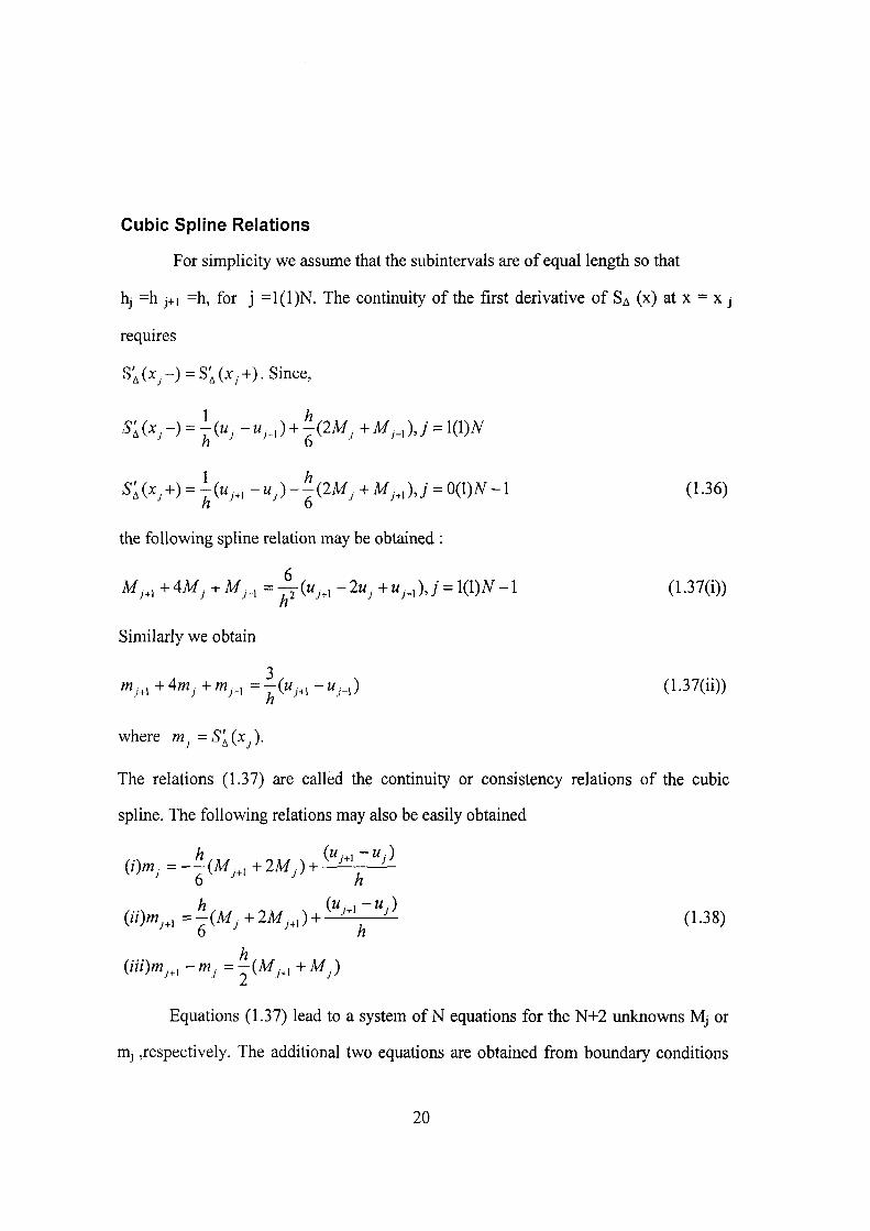
Cubic Spline Relations

For simplicity we assume that the subintervals are of equal length so that

hj =h j+i =h, for j =1(1 )N. The continuity of the first derivative of SA (X) at X = X J

requires

S;(x^-) = S;(x^+). Since

1 . . h

h 6

5 ; ( x , + ) - | K . , - w , ) - 7 ( 2 M , + M , . „ ) , ; = 0(l)iV-l (1.36) n o

the following spline relation may be obtained :

M,„ +4Mj+Mj^, ":^^"^^> -2u^+Uj_,),j = \0.)N-l (1.37(i))

Similarly we obtain

3 rrij^, + 4mJ + m^,, = -(w^^, - w ,,) (1.37(u))

where m^ = S'^ (Xj).

The relations (1.37) are called the continuity or consistency relations of the cubic

spline. The following relations may also be easily obtained

h (w,,,-w,) ( z > - - - ( M ^ , , +2M,)+^ ^ ' ''

6 h h (w,,,-w.)

{ii)m^,, = - ( M ^ + 2 M ^ „ ) + ' \ ' (1-38) n n 6' ' ^^" h

Equations (1.37) lead to a system of N equations for the N+2 unknowns Mj or

mj ,respectively. The additional two equations are obtained from boundary conditions

20

on M or m. The resulting tridiagonal system for Mj or my is diagonally dominant and

may be solved by an efficient algorithm, Ahlberg et al [2]. Therefore, given the values

Uj the equations (1.37) with appropriate boundary conditions form a closed system for

Mj or mj and with (1.34) or (1.35) the values SA (X) can be found at all intermediate

locations.

1.8 Parametric Cubic Spline Functions

Definition 1.2

A function SA (X,T) of class C [a, b] which interpolates u(x) at the mesh points

{xj}, depends on a parameter T , and reduces to cubic spline SA(X), in [a, b] as T-> 0, is

termed a parametric cubic spline function. Since the parameter x can occur in iS" (x, r)

in many ways, such a spline in not unique. The three parametric cubic splines derived

from cubic spline by introducing the parameter in three different ways are termed as

'cubic spline in compression','cubic spline in tension' and 'adaptive cubic spline'.

1.8.1 Cubic Spline In Compression

If S^ (x, T) is a parametric cubic spline satisfying the differential equation

Sl{x,z) + zS,{x,x) = [Sl {x^_,, r) + zS, (x,_,, r)] ^ ^ + hj

,_ (1.39)

where x€[xj_^,Xj],S^(Xj,T) = Uj,hj =Xj ~XJ_^ and T>0 then it is termed cubic

spline in compression (see Aziz [9], Khan [68]).

Solving the differential equation (1.39) and using interpolatory conditions at x j

and X j.i to determine the constants of integration, we get after writing to = /j Vr,

21

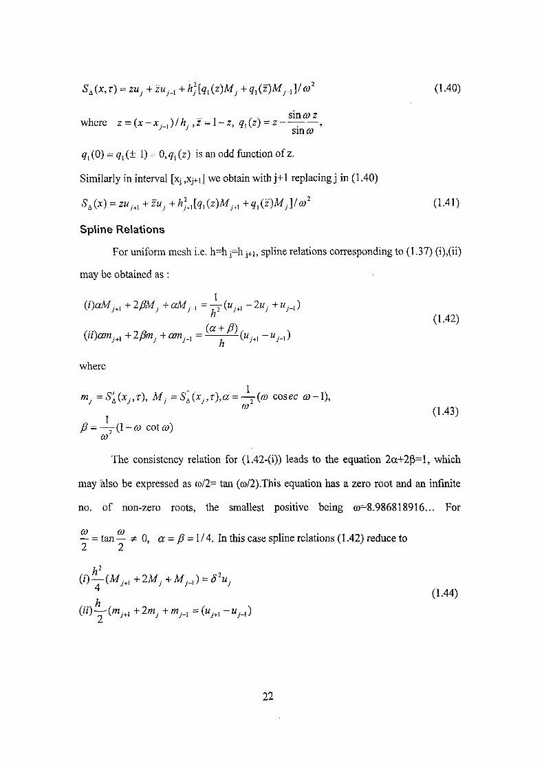
S^{x,T) = zuj + zuj_, + h][q,{z)M^ + q,{z)M j_,y co' (1.40)

sin (O z where z = (x-x. .)lh, ,z -\-z, qAz)~ z-—_ ,

•'" ^ sin 6;

^, (0) = ^, (± 1) = 0, , (z) is an odd function of z.

Similarly in interval [xj ,Xj+i] we obtain with j+1 replacing] in (1.40)

S,{x) = zu^^,+zu^ +h'j^,[q,{z)Mj^, +q,iz)Mj]/o)' (1.41)

Spline Relations

For uniform mesh i.e. h=h j=h j+i, spline relations corresponding to (1.37) (i),(ii)

may be obtained as :

(/>M^„ +2fiMj +ccMj_^ =-7T(«V>I -2UJ+UJ_,)

(a+B) ^^'^^^

{ii)canj^, +2j3mj+amj_^ = ^^^ i^j^x ~^j-\)

where

rrij =S'^(XJ,T), MJ =^ Sl{Xj,T),a = -^{(D cosec ca-l),

J ^ (1.43) yff = — y ( l - < y COlCO)

(O

The consistency relation for (1.42-(i)) leads to the equation 2a+2p=l, which

may also be expressed as a)/2= tan (©/2).This equation has a zero root and an infinite

no. of non-zero roots, the smallest positive being ©=8.986818916... For

— = tan — 9i 0, or = y9 = 1 / 4. In this case spline relations (1.42) reduce to

( 0 ^ ( M , „ + 2 M , + M , . , ) = J \ . ^ (1.44)

(") — (rrij.i + 2mJ + mj_, = {Uj,, - Uj.,)

22

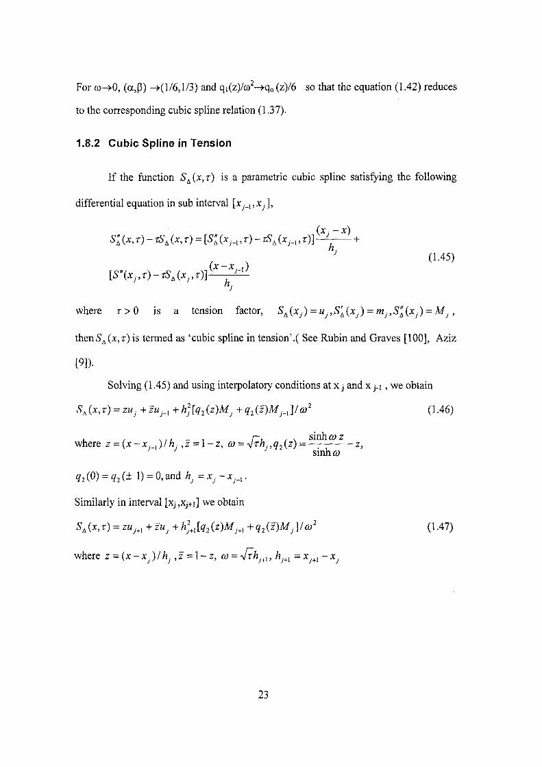
For co->0, (a,P) ->(l/6,l/3) and qi(z)/co ->-qo (z)/6 so that the equation (1.42) reduces

to the corresponding cubic spline relation (1.37).

1.8.2 Cubic Spline in Tension

If the function S^ (x, r) is a parametric cubic spline satisfying the following

differential equation in sub interval [x^_,,Xj],

S: (X, r) - TS, (X, T) = [S: (xj_,, r) - r^, (x,_,, r)] ^ ^ +

, , (1.45) ( x - x , ,)

where r > 0 is a tension factor, S {Xj) = Uj,S'^{Xj) = mj,S'l{Xj) = Mj,

then5^ (x,r) is termed as 'cubic spline in tension'.( See Rubin and Graves [100], Aziz

[9]).

Solving (1.45) and using interpolatory conditions at x j and x j-i , we obtain

S^ix,T) = zu^ -^zu^^^ +h^[q^(z)Mj +q^(z)Mj_J/o)^ (1.46)

where z = (x-x _,)//? ,2 = l - z , Q} = -fvh,,q2{z)~ z, sinh CO

q^ (0) = q^ (± 1) = 0, and h^ = x^ - x^.,.

Similarly in interval [xj ,Xj+i] we obtain

S^{x,T) = zUj,^+zUj+h^Jq,(z)Mj,^ +q,{z)Mj]/o)' (1.47)

where z = (x-Xj)/hj ,z = l-z, a- -Jrhj^^, hj^^ = x .j -Xj

23

Spline Relations

For uniform mesh i.e.,h=h j=h j+i, the following spline relations are obtained:

(0«M,„ +2PM^ +aM^_, -^S'uj (1.48)

where a = —r-(l-fl; cosec h co),/3 = —z-(o} coth CD-I),ca = h^fT 0) 0)

v/heno) ^0,(oc,/3)^ (1/6,1/3), and q2{z)/co^ -^qQ(z)/6, so that the equations

(1.46), (1.47) and (1.48) reduces to the cubic spline relations.

1.8.3 Adaptive Cubic Spline

If the function S^ (x, co) is a parametric cubic spline satisfying the following

differential equation

aSl{x,(o)-bS\{x,(o) = '^^^{aM J -bm^) + '^^(aMj_, -bm.,) (1.49) hj hj

where Xj_^ <x<Xj, a and b are constants,

S'^ (Xj,(o) - nij, S'^ (Xj,co) = Mj, hj = Xj - x^_,, and a)>0, then S^ (x,co)

is termed as 'adaptive cubic spline'.

Solving (1.49) and using the interpolatory constants S^ (;c _,, co) = w ,,,

S^ (Xj, co) = Uj, we have

S,{X,CO) = Aj + B^e^' --^[p,(COz)(M, --m^)] + \[p,(-coz)(M^_, -~mj_,)] CO hj CO hj

(1.50) where

x-x,_, bh z = —,<y = —-,z = \-z,p2(z) = l + z + z^

h ' a • ' - -

24

0) hj

(D hj

7 2

6J 2 hj 2 hj

The function S^(x,ft») on the interval [xj, Xj+i] is obtained with j+1 replacing j in

equation (1.50).

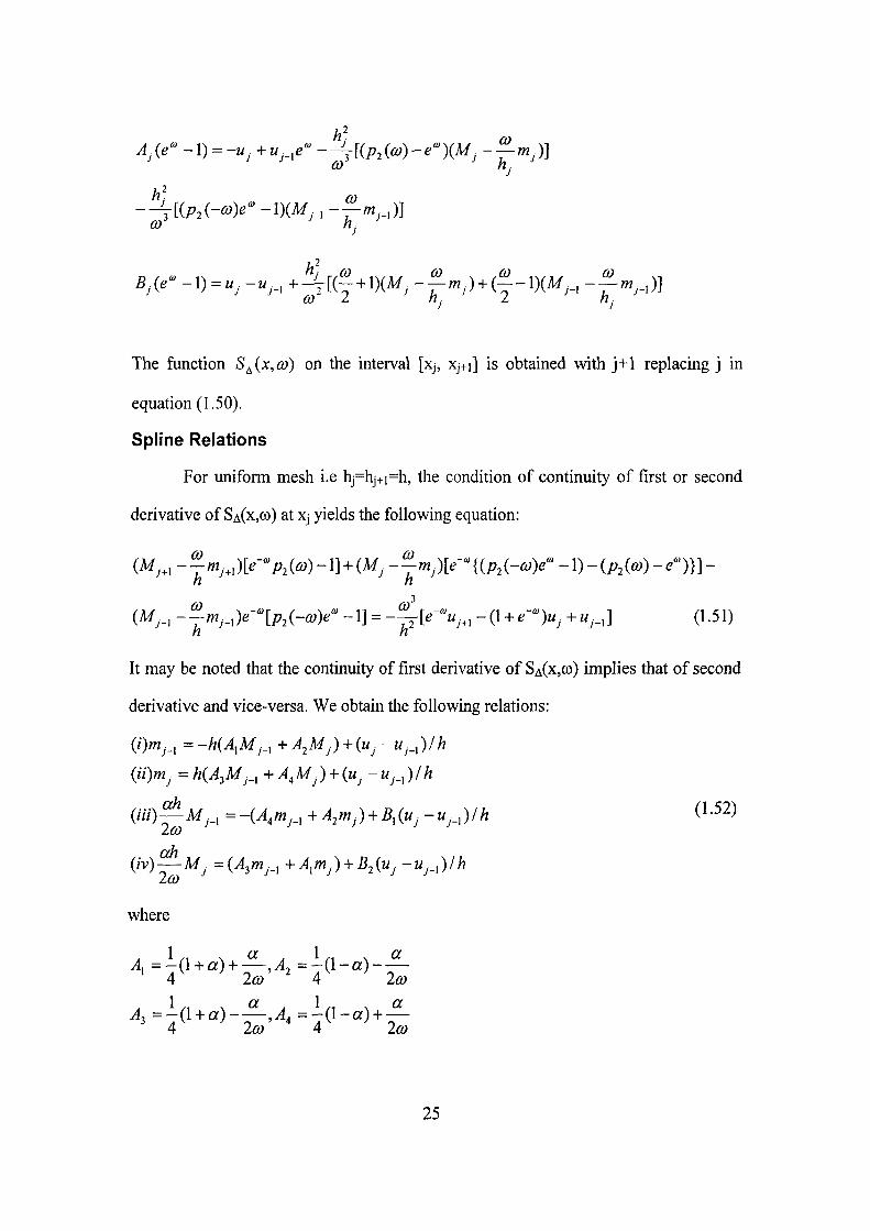
Spline Relations

For uniform mesh i.e hj=hj+i=h, the condition of continuity of first or second

derivative of SA(X,(O) at Xj yields the following equation;

h h

iMj_, -^m^_^)e~'"[p,(-o))e^ ~l] = - ^ [ e ^ w , ^ , - ( l + . - ) w ^ +j.._,] (1.51)

h h

It may be noted that the continuity of first derivative of SA(X,©) implies that of second

derivative and vice-versa. We obtain the following relations:

(/)m^_, = -hiA^Mj_, + A^Mj) + (w - w .,) / h

(ii)mj = h(AjMj_y + A^Mj) + (w - w _,) / h

m^Mj_, =-(A,mj_, +A,m^) + B,(u^ -u^_,)lh (1-52) ICO

cch {iv)~-M = ( ^ 3 ^ 1 + A,mj) + B^{u- - w _ , ) /h

10}

where

A, =-{\ + a) + —,A, = " ( ! - « ) - — 4 2<y 4 Ico

1 / 1 -. (^ A 1 / 1 N or A,=-a + a)-—,A, = - - ( l - a ) + —-4 2a) 4 2o)

25

1 1 O

B^ =—(l-a),B2 =—(l + a),a = coth 2 2 2 0)

We also obtain

2 h'[A,Mj^, +iA, +A,)M^+A,M^_,] = S'u^ (1.53)

,M^„ - (5, + 2)M . + B,Uj_, = M^w^.^, + iA^ + A,)mj + A^mj_^ ] (1.54)

For co-»0 (i.e. bh/a^O), then we have a =0,a /(o=l/6, Ai=A4=l/3, A2=A3=l/6,

Bi= -B2 =1/2, and the spline function given by (1.50) reduces into cubic spline.

1.9 Quartic Spline Functions

(I) Let u (x) be a sufficiently differentiable function and u (x) be an approximation

to u(x) obtained by a 'quartic spline' Qj(x) passing through the points (xj Uj )and (xj+i,

Uj+i).The spline function S(x) can be written in the form of a quartic polynomial Qj(x)

in each subinterval [Xj,Xj+i]along with the requirement that S(x)e C [a,b],

(See Usmani [123]). We write Qj(x) in the form

Qj{x) = aj{x-Xjy+bj{x-Xjf+c^{x-Xjf+dj{x-Xj) + ej, j = 0(l)N-l

(1.55)

The set of quartic polynomials, using a different polynomial in each subinterval

[Xj Xj+i] defines a smooth approximation to u(x). We further require that the values of

the first, second and third order derivatives be the same for the pair of quartics that join

at each point (xj,Uj). We determine the five coefficients of (1.55) in terms of

Uj^^ij,mj,Mj^^i^,Tj and Fj ,, where we write

e ; (x , )=mj, Q:(XJ,„,) =MJ,,„,

Qr(xp=T., Qr^(x,,„,) =F.,„, Using the five equations namely

26

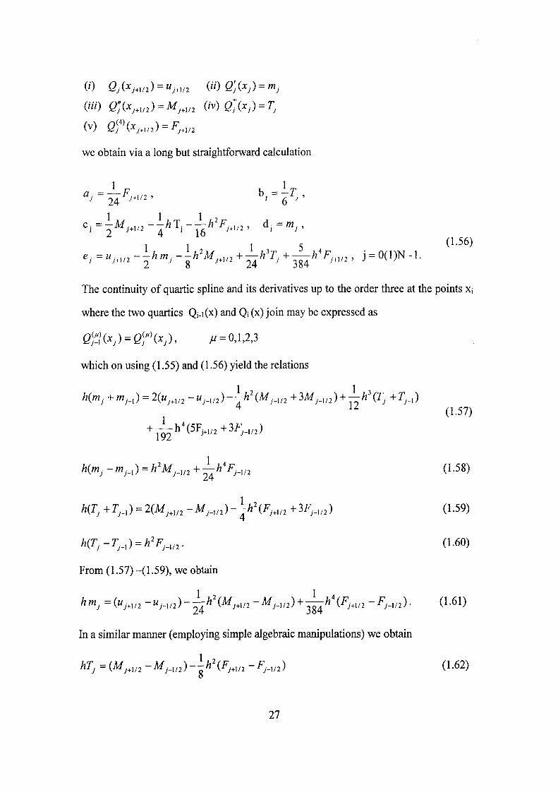
(0 Qj(Xj,v2)^J^j.u2 (ii) Qj(Xj) = mj

(iii) Q]{Xj,,n) = Mj,,,, iiv)Q";(Xj) = T^

(V) Qr(^J.U2) = Fj.U2

we obtain via a long but straightforward calculation

1 1 1 5 (^-^6)

The continuity of quartic spline and its derivatives up to the order three at the points Xj

where the two quartics Qi-i(x) and Qi (x) join may be expressed as

Q'j1(Xj) = Q'/\xj), M = 0,1,2,3

which on using (1.55) and (1.56) yield the relations

(1.57)

h{m^ -m^_,) = h'Mj_,,,+^^h'F^_,„ (1.58)

/z(7; +r , . , ) = 2(M^„/, -Mj_,,,)-h\Fj^,„ +3F^.,/,) (1.59)

h(Tj-T^_,)^h'Fj_,,,. (1.60)

From (1.57) -(1.59), we obtain

1 2 1 4

hmj=(Uj,,,,-Uj_,„)-^h iMj^,,,-Mj_y,) + —h (Fj,,,, - Fj_y,). (1.61)

In a similar manner (employing simple algebraic manipulations) we obtain

hTj ={Mj,,,, -M.^,,,)-h\Fj,,,, -F,., ,^) (1.62)

27

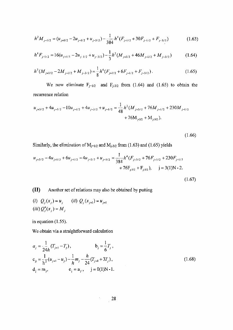
h'M^_,,, =(",. , /2 -2W;-,/2 + « , - 3 / 2 ) - ^ ^ ' ( ^ , > , / 2 + 30F,_,/2 + ^,-3/2 ) (1-63)

, 1 , h F^.,/2 = 1 6 ( M ; „ / 2 -2W^_,/2 + W , - 3 / 2 ) - 3 ^ (^y.i/2 +46M^_,/2 +M^_3/2) (1.64)

h\M^^,,, -2M^_,,2 +M^_3, , )^ iA\F^ . , , , , +6F^..„, +F , . 3 , , ) . (1.65)

We now eliminate Fj+1/2 and Fj.3/2 from (1.64) and (1.65) to obtain the

recurrence relation

1 , "y+3/2 +4w,>,/2 -10",-l/2 +4w,-3/2 + "7-5/2 = ^ ^ (^,+3/2 +76M^„/2 +230M^_,/2

+ 76Mj.3/2+Mj.5/2).

(1.66)

Similarly, the elimination of Mj+1/2 and Mj.3/2 from (1.63) and (1.65) yields

",.3/2 -4",>,/2 + K - I / 2 -4Wy-3/2 +"y-5/2 = —^'(^y>3/2 + 76F^.l/2 + 230F,_,/2

+ 76F^-3/2+F,.5/2X J - 3 ( l ) N - 2 .

(1.67)

( I I ) Another set of relations may also be obtained by putting

(0 Qj i^j ) = "y ("•) Qj (^;+i) = "y+1

("oe;(^,)=M,

in equation (1.55).

We obtain via a straightforward calculation

' ^ = ]^(".>. - " . ) - ^ ' " v - ^ ( ^ . > . + 37;), (1.68)

A.=m., t.=Uj, j = 0 ( l )N- l .

28

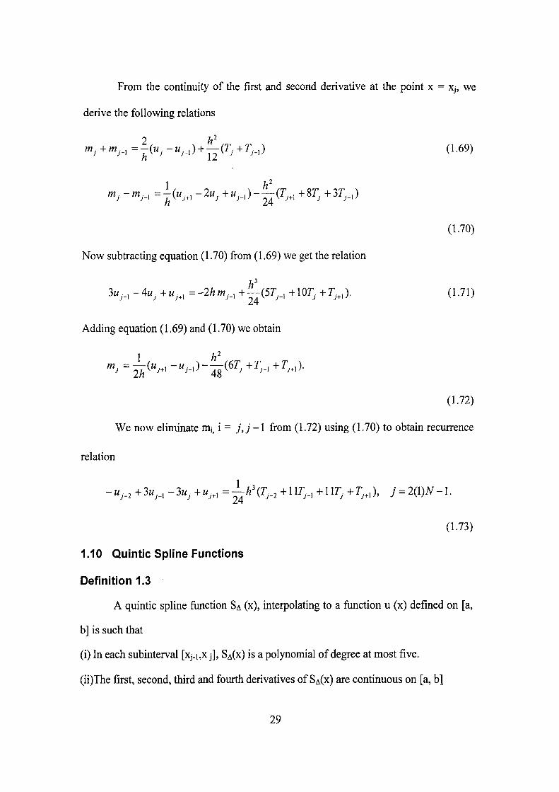
From the continuity of the first and second derivative at the point x = Xj, we

derive the following relations

m^ +m^_, =|(z,^ -„^_,) + : ^ ( r , +r^.,) (1.69)

1 h^

h' ^^' ' '-" 24

Now subtracting equation (1.70) from (1.69) we get the relation

(1.70)

lu^_, -Au^ +w^,, =-2hm^_, ^YA^^^H +10^.+^...)- (1-71)

Adding equation (1.69) and (1.70) we obtain

'"^ " 2A ^"^ ' " "^-' ~ 48 ^ •' " ^-' ^ ^-''' -*•

(1.72)

We now eliminate mi, i = 7,7-1 from (1.72) using (1.70) to obtain recurrence

relation

- uj_, + 3uj_, - 3uj + «,„ =j^h'(r,., +1 ir,_, +1 IT; + T;,,), j = 2(1)N - 1 .

(1.73)

1.10 Quintic Spline Functions

Definition 1.3

A quintic spline function SA (X), interpolating to a function u (x) defined on [a,

b] is such that

(i) In each subinterval [xj.i,x j], SA(X) is a polynomial of degree at most five.

(ii)The first, second, third and fourth derivatives of SA(X) are continuous on [a, b]

29

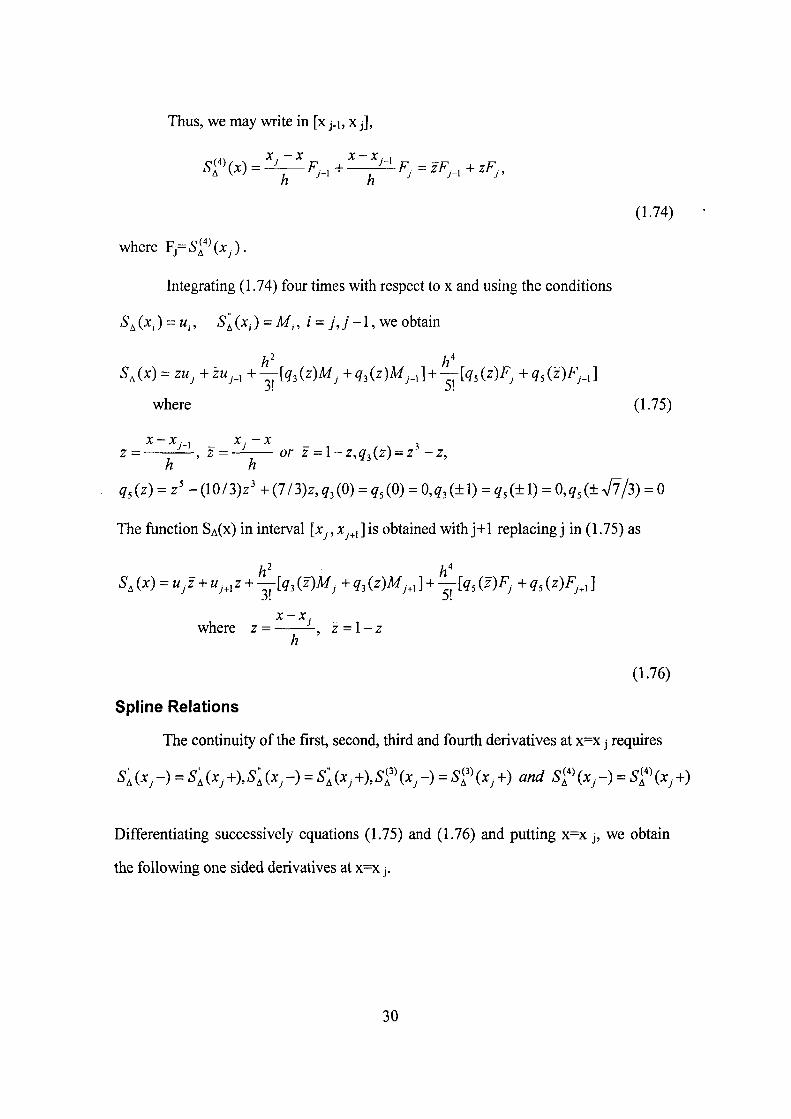
Thus, we may write in [Xj.i, x j],

(1.74)

where FrS['\Xj).

Integrating (1.74) four times with respect to x and using the conditions

S^(x,.) = w,., Si(x^) = M,, i = j,j-\,v^eobtain

S^(x) = zUj+zUj_, +—[q,(z)Mj+q,(z)M^_,] + — [q,(z)Fj+q,{z)Fj_,]

where (1-75)

z^———, z=—;— or z = l-z,q^(z) = z -z, h h

^3(z) = z'-(10/3)z^+(7/3)z,^3(0) = 3(0) = 0,^3(±l) = 3(±l)-0,^,(±V7/3) = 0

The function SA(X) in interval [Xj, x , ] is obtained with j+1 replacing j in (1.75) as

S^ (x) = UjZ + Uj^,z + —[q, (z)Mj + q, (z)Mj,, ] + —[q, (z)F^ + q, (z)Fj^, ]

x-x. where z = -, z = l-z

h

(1.76)

Spline Relations

The continuity of the first, second, third and fourth derivatives at x=x j requires

S, (X, -) = S, (x^ +), Si (x^ -) = Si (Xj +),5f (Xj -) = 5 f (Xj +) and 5f ^ (Xj -) = S'^' (Xj +)

Differentiating successively equations (1.75) and (1.76) and putting x=x j , we obtain

the following one sided derivatives at x==x j .

30

h o 360

h ' 6 360 Q)Sl{x^-) = M^=Sl{x^+)

i4)S'^\x^-) = i ( M , -M,_,) + (F^_, + 2F^) n 0

« o

(6)5l^^(x,-) = F^.=5l^^(x^+) (1.77)

The continuity of first derivative implies

M,,, +4M^ +M^., =;^(",>, -2u, +w,_,) + ( 7 F ^ „ +16F^ +7F^_,),7 = 1(1)A^-1

(1.78)

and the continuity of the third derivative implies,

M^,, -2M^ +M^,, = ^ ( F , „ +4F^ +F,_,), ; =l(l)iV-l

(1.79)

subtracting (1.79) from (1.78) and dividing by 6 we obtain

(1.80)

Elimination of Mj's between (1.79) and (1.80) leads to the following useful relation:

120 F^,, +26F^,, +66F, +26F,_, +F^_,= ^{Uj^,-4uj^, +6uj -4w,_, +Uj_,),J = 2(\)N-2

(1.81)

The following additional spline relations may be obtained

31

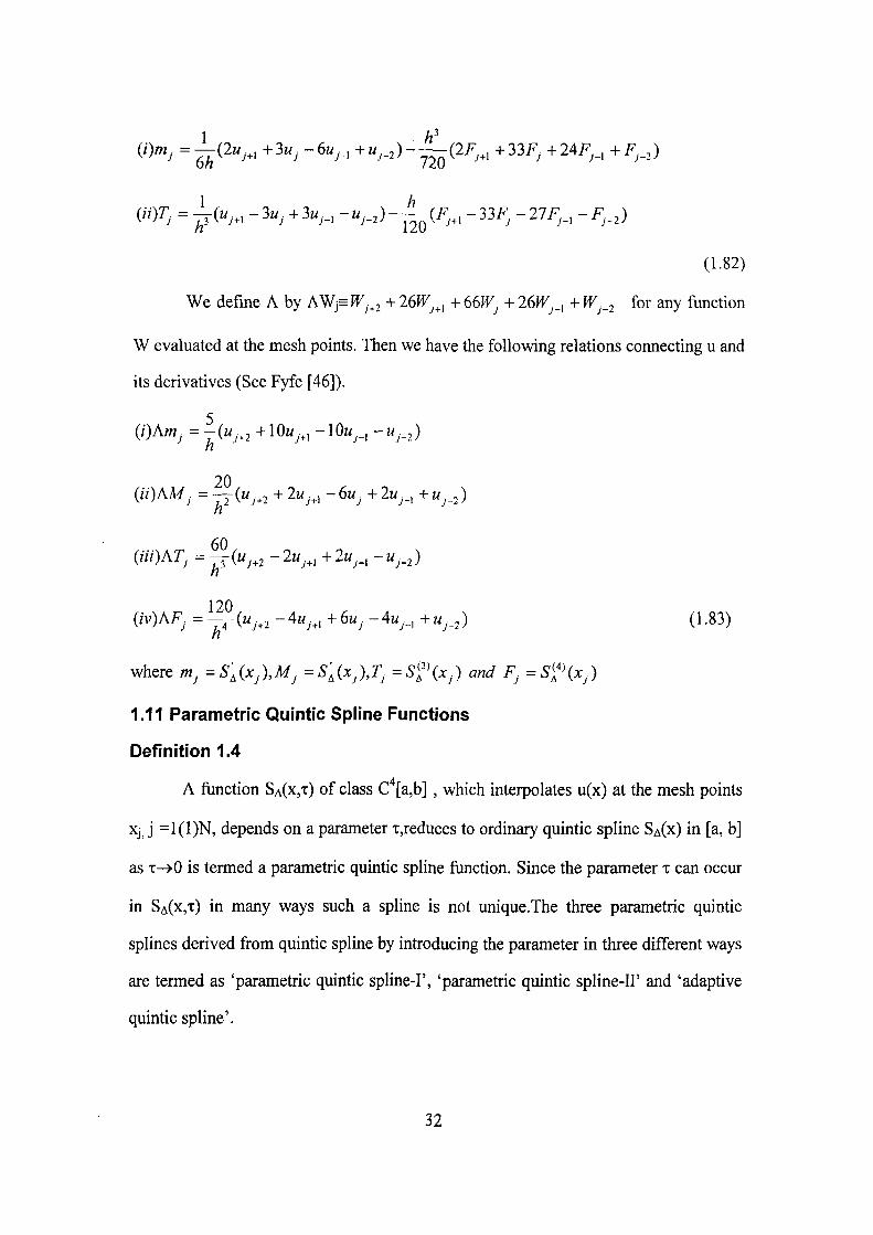
07)7;. = ^(^v^,, -3«,. +3.^._, - „ ^ . , ) - l - ( F . , -33F, -27F,_, -F^_,)

(1.82)

We define A by AWj ff ^ + 26H ,„ + 66PF + 26Wj_, + Wj_^ for any function

W evaluated at the mesh points. Then we have the following relations connecting u and

its derivatives (See Fyfe [46]).

{i)Amj =-7("y+2 +10"v>i -10"y-i ""y-2)

20

(iiOATj =^(«y .2 -2w,,, +2w^_, -u^_,)

120 (iv)Ai ^ = ^ K > 2 -4",>, +6w, -4w .„, +«._,) (1.83)

where w, =5 , (x , ) ,M, =-S;(x^),r, =5f ' (x . ) o«^ F, =Si'\xj)

1.11 Parametric Quintic Spline Functions

Definition 1.4

A function SA(X,X) of class C [a,b] , which interpolates u(x) at the mesh points

Xj, J =U1)N, depends on a parameter T,reduces to ordinary quintic spline SA(X) in [a, b]

as T->0 is termed a parametric quintic spline function. Since the parameter T can occur

in SA(X,T) in many ways such a spline is not tinique.The three parametric quintic

splines derived from quintic spline by introducing the parameter in three different ways

are termed as 'parametric quintic spline-I', 'parametric quintic spline-IP and 'adaptive

quintic spline'.

32

1.11.1 Parametric Quintic Spline-I

If SA(X,T)= SA(X) is a parametric quintic spline satisfying the following

differential equation in the interval [x j.i, x j],

-'(4)/'v-^ _ L - ^ 2 e (2) . 2 » y \ •*• """j-l S^^\x) + T'Sr{x)^{Fj+T'M^)^^ + {F^_,+T'Mj_,)

X. - X

h h

= QjZ + Qj-^z, (1.84)

where Qj= Fj +x Mj , 5]^(x^) = M^, S'-/^\xj)= Fj and x >0 then it is termed

'parametric quintic spUne-F.

Solving the differential equation (1.84) and determining the four constants of

integration from the interpolatory conditions at x j and x j.i, we obtain

/ j2 ^

S^(x) - zu + zw , + —[q,iz)Mj + q,(z)Mj_i] + ( - ) ' 3! (W

0) ^ , ( Z ) - < , , ( Z ) ] F ^ +

93(z)-9,(z) ]F^_, (1.85)

where q3(z) and qi(z) are defined in section (1.7) and (1.8.1) respectively.

In the same manner in [Xj, x , ] we obtain

S^ix) = zuj + zuj,, + —[q,(z)Mj + q,{z)M J + ( - ) ' 3! 0)

CO —q^{z)-qx{z) ] y+i +

6)

0)

3! q,{z)-q,(z) ]F^ (1.86)

Spline Relations

Continuity of the first and second derivatives implies that

n

(ii) M^„ - 2Mj + Mj_, = h' (oFj,, + 2J3Fj + aF._^ (1.87)

33

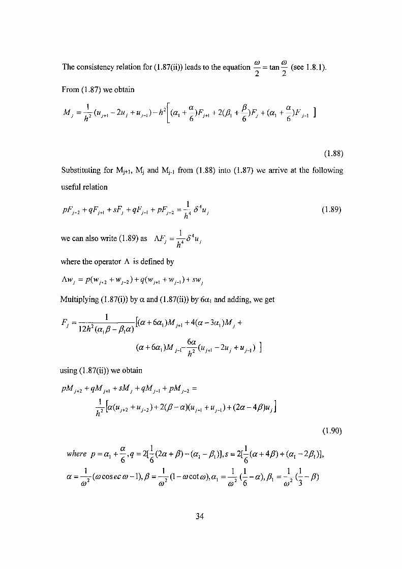
The consistency relation for (1.87(ii)) leads to the equation — = tan— (see 1.8.1).

From (1.87) we obtain

M^ = ^ ( « , . , -2u^ +u^_,)-h' (a, + | )F^„ +2(J3, + | ) F ^ +(«, + | )F^_ , ]

(1.88)

Substituting for Mj+i, Mj and Mj.i from (1.88) into (1.87) we arrive at the following

useful relation

Pf^j.2 + 9^,., + sFj + qF^_, + pF^_, = ^S'u^ (1.89)

we can also write (1.89) as AF, = —rS'^u,

where the operator A is defined by

Aw. = p(Wj^^ + Wj_2 ) + q{-Wj,, + Wj_^ ) + SWj

Multiplying (1.87(i)) by a and (1.87(ii)) by 6a\ and adding, we get

^J ^ , 0 , 2 , \ n J ( « + 6a,)M,„ + 4 (a -3a , )M. + 12/2 (a,y^-y^,a) ^

(a + 6a,)M^..,-^(w^.,, -luj +M^._,) ]

using (1.87(ii)) we obtain

— [a(Uj,, + Uj_, ) + 2iP- a){Uj,, + «^.,) + (2a - 4j3)Uj ] n

(1.90)

where p = a,+^,q = 2[\{2a + P)-{a,-p,)],s = 2[Ua + A/3) + {a,-2p,)], o 0 6

—jiacosec co-\),p ^ -^{\-(ocoXQ)),a^ = - y ( - - a ) , y 9 , = - Y ( T -(y 6J CO 6 CO i

34

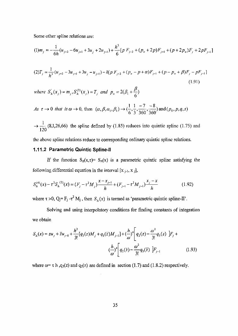
Some other spline relations are:

1 h' O K =~-g^^"^-2 -6« ,„ +3«^ +2w,.,) + y [ p F , , 2 +{p„+2p)F^^, +(p + 2p„)Fj+2pFj_,]

{2)T^ = (w ,, - 3M^„ + 3w - Uj_,) - h[p Fj,, +(p„-p + «)F^„ + (p - P„ + /?)F, - pF^_, ]

(1.91)

where S,(x^)^m^,S^^\x^)^T^ and p„ =2(/?, + | )

1 1 — 7 —8 As T^O that isa^O, then (a,y9,«,,y?,)-^ ( - , - , -—, -—) and (;7(,,/>, 9,5)

o i JOU ioU

-> (8,1,26,66) the spline defined by (1.85) reduces into quintic spline (1.75) and

the above spline relations reduce to corresponding ordinary quintic spline relations.

1.11.2 Parametric Quintic Spline-il

If the function SA(X,T)= SA(X) is a parametric quintic spline satisfying the

following differential equation in the interval [x j.i, x j],

Si'\x) - T'S,''\X) = (Fj - r'Mj)^^^ + (F^_, - r ^ M ^ _ , ) ^ (1.92) •^ h h

where T >0 , QJ= FJ -X^ MJ , then S^{x) is termed as 'parametric quintic spline-II'.

Solving and using interpolatory conditions for finding constants of integration

we obtain

S^(x) = zu + zu , + —[q,{z)M + q,{z)M ,] + ( - ) ' 3 ! ^ CO

a' ?2(^)-Y^3(^)K +

0)

.-. co' q^(^)-—q^(^) K , (1-93)

where co= x h ,q3(z) and q2(z) are defined in section (1.7) and (1.8.2) respectively.

35

Spline Relations

Continuity of the first and third derivatives yields the following spline relations

(1.94)

Using (1.94) we obtain

(1.95)

Substituting for Mj+i, Mj and Mj.i from (1.95) into (1.94) we arrive at the following

useful relations

pF,,.,F,„.sF,.,f,_,.pF,_,.^S'u, (1.96)

Multiplying (1.94(i)) by a and (1.94(ii)) by 6a\ and adding, we get

Fj - , , , 2 , \ o J ( « + 6a,)M^„ + 4(a-3a,)M^ +

(a + 6a,)Mj_-—(Uj,, -2uj +w^_,) ]

using (1.94(ii)) we obtain

pMj^2 +9^i+i +sMj +qMj_y +pMj_2 =

-^ [a{uj,2 + Uj_2 ) + 2(j3- a){Uj,, + M ., ) + (2a- Ap)Uj ]

Some other spline relations are:

(1.97)

(l)m, = - ^ K > 2 - 6 " ; . , +3M, +2«,_,) + [/?7^,,2 +(;^. +2p)/^;., +{p + 2p,)Fj+2pFj_,]

36

(2)r^ =^(^j.2 -3«,. , +3uj -Uj_,)-h[pFj,, +{p„-p + a)Fj,, +(^p-p^+p)F. - pF^_,]

(1.98)

where p = a,+^,q = 2[U2a + l3)-{a,-p,)],s^2[\{a + Ap) + {a,-2p,)], 6 6 6

—),a = ^ (I-0) cos ech 0)),/3 = — 6 CO CO

Pg =2(/?| +^),a = —^(\-CO cos echo)), p = —^{-\ + o)coihco).

6> 6 Q} i

1 1 — 7 —8 As r^O that is co^O, then (a,/9,«i,y9,)->(-,-,-—,-—)and(/>o,/7,^,5)

6 3 360 360

-^ (8,1,26,66) the spline defined by (1.93) reduces into quintic spline (1.75) and

the above spline relations reduce to corresponding ordinary quintic spline relations.

1.11.3 Adaptive Quintic Spline

If the function SA(X,CD) is a parametric quintic spline satisfying the following

differential equation in the interval [x j.i, x j],

aSf(x,co)-bS,''\x,a)) = (aF^ -bTj)^^^ + {aF^_, -bT^_,)^^ ^ 99^

where x e [x j.i, x j ],Sf^{Xj,o)) = Tj, S[*\xj,co) = Fj, co = bh/a >0 ,a,b are constants,

then Sf\x,Q)) is termed as 'adaptive quintic spline'.

Solving (1.99) and using the interpolatory conditions we obtain

S^ (x,CO) = UjZ + u^,,z + A,[<z5, (z) + 2(z)]M. -k,[^,(z)e" + <t>-,(z)]M^_, +

K(l,-x V^^ i^)iP2 i-OJ)e'" -1) + /I2 {P2 {-(O) - \)<f>2 (z) - zp, {-co) + p, i-o^) -z] (1.1 GO)

where

37

^ , z = l - z , Q^=Fj--T^, oj = —, M^=Sl(Xj,CD), h a a

A = (e'"-\y' and p^(t) = \ + t + ~ + --+—. ^ 2! N\

The function5"^(x,(y)on the interval [x^,x^^]]is obtained with j+1 replacing j in

(1.100).

Spline Relations

The condition of continuity of first and third derivative of SA(X,G)) at Xj yields

the following equations:

(0 (",» - 2"; + Uj_,) = k,Mj^^ + k^Mj + k,Mj_^ + k^qJ^^ + k^qj + k,qj_^

(/•/•) M.„ -{l + e^Mj +e"M,_, = A,{[l-A(p,M-l)k^„ +[A(p,(«)e'" -p , («))-3k,

+ [A(p,(-6;)-l)e^+lk,_,}/A, (1.101)

where k, =ie'" -p,{cD)A,), k, =[e'"{p,io})-3) + (3-p,(-CDm„ k, ^[e"p,{-co)-l]A„ 3 2

k,=-X,[~-ip,icD)-e'') + X(p,i(o)-m + o)-e'') + p,(co)-co-\],

k,=A,[-2o} + ^ + Aco\l-^)(l+ €")], and k, = A J - ^ ( p 2 ( - f i ; ) e ' " - 1 ) + 3 ^ 4 ' " '^' ' " ° "^ 2

/l(p, (-co) -!)[(« - Oe-" +1] + p , (-0)) + Q}-\]

Since the condition for the continuity of the fourth and higher derivatives is same as

that of the third derivative it follows that derivatives of all order for the adaptive

quintic spline are continuous.

38

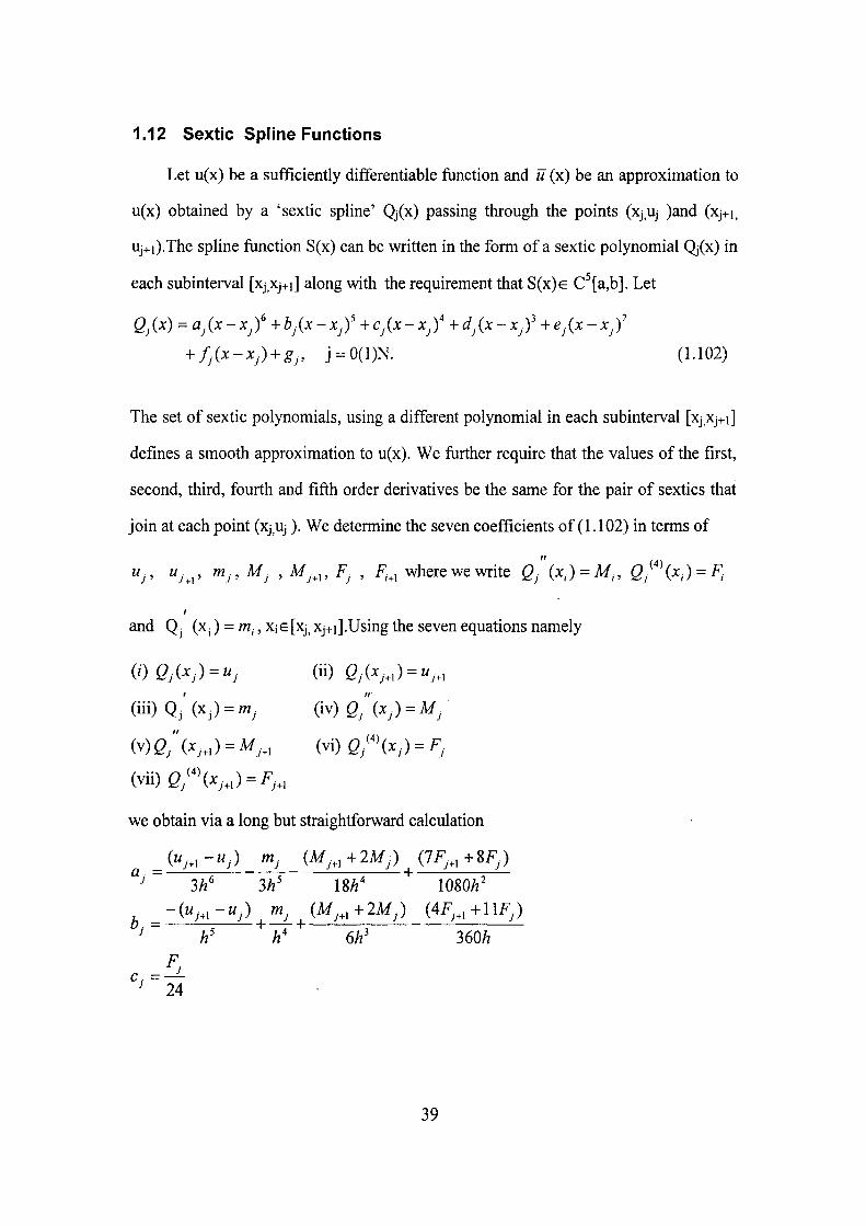
1.12 Sextic Spline Functions

Let u(x) be a sufficiently differentiable function and u (x) be an approximation to

u(x) obtained by a 'sextic spline' Qj(x) passing through the points (xj Uj )and (xj+i,

Uj+i).The spline function S(x) can be written in the form of a sextic polynomial Qj(x) in

each subinterval [xj Xj+i] along with the requirement that S(X)G C^[a,b]. Let

Qj(x) = aj(x - Xjf + bjix - Xjf + Cj{x - x^)' + dj{x - Xj)^ + e /x - x^)'

+ fM-Xj) + g^, j = 0(l)N. (1.102)

The set of sextic polynomials, using a different polynomial in each subinterval [xjXj+i]

defines a smooth approximation to u(x). We further require that the values of the first,

second, third, fourth and fifth order derivatives be the same for the pair of sextics that

join at each point (xj,Uj). We determine the seven coefficients of (1.102) in terms of

" (4')

" y "y.i' ^j^^j ^^j^x^Fj ' / >, where we write Qj (x,) = M,, Q^ (x,) = /^

and Qj (Xj) = w ,Xie[xj^Xj+i].Using the seven equations namely

(0 Qj (^,) = Uj (ii) QJ {XJ^, ) = Uj^,

(m)Q.(x^) = mj (iv)Q"(Xj) = Mj

(v)Q"iXjJ = M^^, {Vx)Q^'\x^) = F^

(vii)(2;'"(x^.„) = F,„

we obtain via a long but straightforward calculation

^ ^ (»,„ -Uj) nij (M,„ +2M,) ^ (7F,„ +87^^)

^ ^ - ( » ; . . - ^ ) , ^ y , (^ ; . .+2M^.) (4F^,,+lli^,)

' h' h' 6h' 360/z

' 24 c = '

39

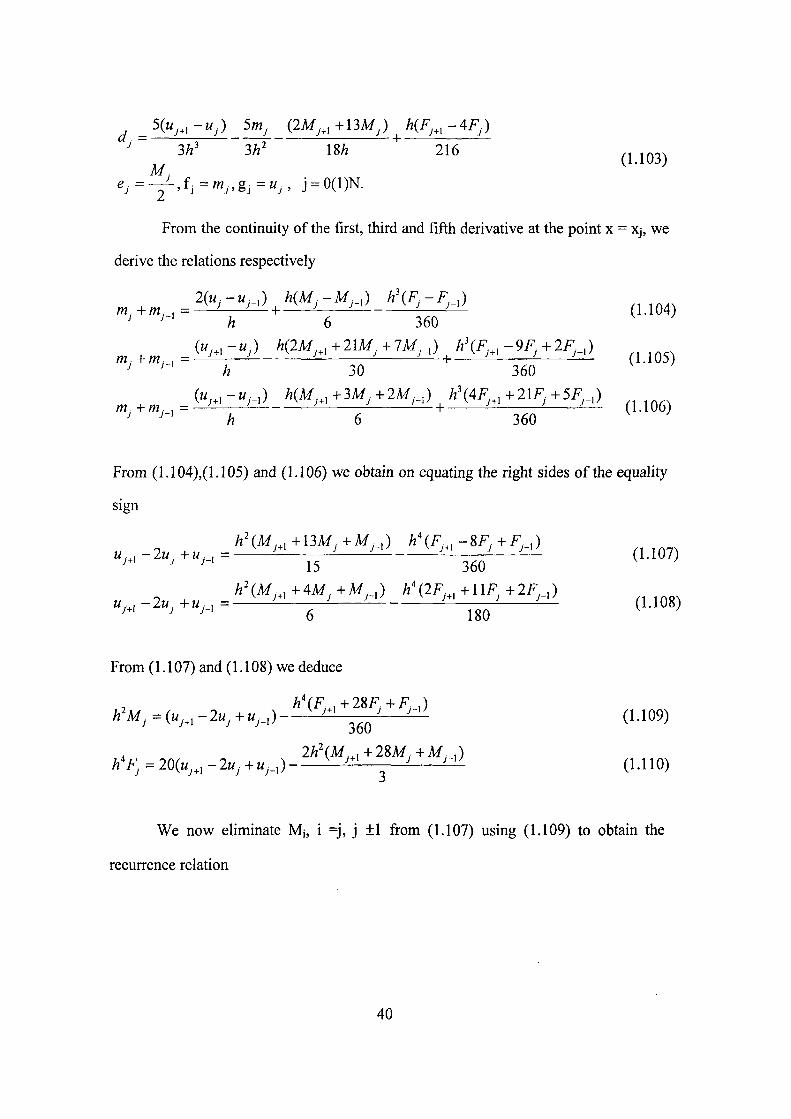
' 3/2' 3/2' I8/2 " 216 .J ^Q^.

From the continuity of the first, third and fifth derivative at the point x = Xj, we

derive the relations respectively

2{Uj-u^_,) h{Mj-M^_,) h\Fj-F^_,) m.+m,,=— —H — (1.104)

' '""' /? 6 360 •J, (»^.„ - u ^ ) /z(2M^„ + 21M^ + 7M^_,) ^ h\Fj,, -9Fj + 2F^..)

h 30 ^ 360

360

m . + m . , , ^ ^ ^^\ ' - ^ ^-^—:^ vzi + _ jLJ lL__J Zdl (1.105)

From (1.104),(1.105) and (1.106) we obtain on equating the right sides of the equality

sign

h' (M . , + 13M, + M . , ) h' (F . , - 8F,. + F ,) w , . -2w,+w, , = ^ '- ^ ^^^J '- '-^ (1.107)

'"' ' '"' 15 360 . 2 , /z^(M,„ +4M,+M,_,) A^(2F^^,+11F^ +2F,_,)

6 180 /.,,, -22/^ +z. ._, = ^ ^" , ^ ^ - ^ " . . . ^ ^ (1.108)

From (1.107) and (1.108) we deduce

;z ' (F. ,+28F,+F, ,) h'Mj ^ (Uj^, -2uj+uj_,) ^ ' 3^Q^ ^"" (1.109)

2/z'(M,.,+28M,+M, ,) h'Fj^20(u^^,-2uj + u^_,)- ' ^ ' ^ ^ (1.110)

We now eliminate Mj, i =j, j ±1 from (1.107) using (1.109) to obtain the

recurrence relation

40

y = 2(l)A^-2, (1.111)

We also obtain the following useful relation

h\M^ 2 +56M,, +246M, +56M,., +M, . , ) u^_, +8«,_, -18«, +8u,„ +«^,3 ^ - ^ ^ i ^ "' 3Q ^ '- '—

(1.112)

For the sake of briefness, we omit error estimates for quadratic, cubic, quartic, quintic,

and sextic splines.

41