CHAPTER ONEtestbank360.eu/...manual-calculus-6th-edition-hughes-hallett.pdfFull file at . 2 Chapter...
94
1.1 SOLUTIONS 1 CHAPTER ONE Solutions for Section 1.1 Exercises 1. Since t represents the number of years since 1970, we see that f (35) represents the population of the city in 2005. In 2005, the city’s population was 12 million. 2. Since T = f (P ), we see that f (200) is the value of T when P = 200; that is, the thickness of pelican eggs when the concentration of PCBs is 200 ppm. 3. If there are no workers, there is no productivity, so the graph goes through the origin. At first, as the number of workers increases, productivity also increases. As a result, the curve goes up initially. At a certain point the curve reaches its highest level, after which it goes downward; in other words, as the number of workers increases beyond that point, productivity decreases. This might, for example, be due either to the inefficiency inherent in large organizations or simply to workers getting in each other’s way as too many are crammed on the same line. Many other reasons are possible. 4. The slope is (1 − 0)/(1 − 0) = 1. So the equation of the line is y = x. 5. The slope is (3 − 2)/(2 − 0) = 1/2. So the equation of the line is y = (1/2)x +2. 6. Using the points (−2, 1) and (2, 3), we have Slope = 3 − 1 2 − (−2) = 2 4 = 1 2 . Now we know that y = (1/2)x + b. Using the point (−2, 1), we have 1= −2/2+ b, which yields b =2. Thus, the equation of the line is y = (1/2)x +2. 7. Slope = 6 − 0 2 − (−1) =2 so the equation is y − 6 = 2(x − 2) or y =2x +2. 8. Rewriting the equation as y = − 5 2 x +4 shows that the slope is − 5 2 and the vertical intercept is 4. 9. Rewriting the equation as y = − 12 7 x + 2 7 shows that the line has slope −12/7 and vertical intercept 2/7. 10. Rewriting the equation of the line as −y = −2 4 x − 2 y = 1 2 x +2, we see the line has slope 1/2 and vertical intercept 2. 11. Rewriting the equation of the line as y = 12 6 x − 4 6 y =2x − 2 3 , we see that the line has slope 2 and vertical intercept −2/3. 12. (a) is (V), because slope is positive, vertical intercept is negative (b) is (IV), because slope is negative, vertical intercept is positive (c) is (I), because slope is 0, vertical intercept is positive (d) is (VI), because slope and vertical intercept are both negative (e) is (II), because slope and vertical intercept are both positive (f) is (III), because slope is positive, vertical intercept is 0 Full file at http://testbank360.eu/solution-manual-calculus-6th-edition-hughes-hallett
Transcript of CHAPTER ONEtestbank360.eu/...manual-calculus-6th-edition-hughes-hallett.pdfFull file at . 2 Chapter...

1.1 SOLUTIONS 1
CHAPTER ONE
Solutions for Section 1.1
Exercises
1. Since t represents the number of years since 1970, we see that f(35) represents the population of the city in 2005. In
2005, the city’s population was 12 million.
2. Since T = f(P ), we see that f(200) is the value of T when P = 200; that is, the thickness of pelican eggs when the
concentration of PCBs is 200 ppm.
3. If there are no workers, there is no productivity, so the graph goes through the origin. At first, as the number of workers
increases, productivity also increases. As a result, the curve goes up initially. At a certain point the curve reaches its highest
level, after which it goes downward; in other words, as the number of workers increases beyond that point, productivity
decreases. This might, for example, be due either to the inefficiency inherent in large organizations or simply to workers
getting in each other’s way as too many are crammed on the same line. Many other reasons are possible.
4. The slope is (1− 0)/(1− 0) = 1. So the equation of the line is y = x.
5. The slope is (3− 2)/(2− 0) = 1/2. So the equation of the line is y = (1/2)x+ 2.
6. Using the points (−2, 1) and (2, 3), we have
Slope =3− 1
2− (−2)=
2
4=
1
2.
Now we know that y = (1/2)x + b. Using the point (−2, 1), we have 1 = −2/2 + b, which yields b = 2. Thus, the
equation of the line is y = (1/2)x + 2.
7. Slope =6− 0
2− (−1)= 2 so the equation is y − 6 = 2(x− 2) or y = 2x+ 2.
8. Rewriting the equation as y = −5
2x+ 4 shows that the slope is −5
2and the vertical intercept is 4.
9. Rewriting the equation as
y = −12
7x+
2
7shows that the line has slope −12/7 and vertical intercept 2/7.
10. Rewriting the equation of the line as
−y =−2
4x− 2
y =1
2x+ 2,
we see the line has slope 1/2 and vertical intercept 2.
11. Rewriting the equation of the line as
y =12
6x− 4
6
y = 2x− 2
3,
we see that the line has slope 2 and vertical intercept −2/3.
12. (a) is (V), because slope is positive, vertical intercept is negative
(b) is (IV), because slope is negative, vertical intercept is positive
(c) is (I), because slope is 0, vertical intercept is positive
(d) is (VI), because slope and vertical intercept are both negative
(e) is (II), because slope and vertical intercept are both positive
(f) is (III), because slope is positive, vertical intercept is 0
Full file at http://testbank360.eu/solution-manual-calculus-6th-edition-hughes-hallett

2 Chapter One /SOLUTIONS
13. (a) is (V), because slope is negative, vertical intercept is 0
(b) is (VI), because slope and vertical intercept are both positive
(c) is (I), because slope is negative, vertical intercept is positive
(d) is (IV), because slope is positive, vertical intercept is negative
(e) is (III), because slope and vertical intercept are both negative
(f) is (II), because slope is positive, vertical intercept is 0
14. The intercepts appear to be (0, 3) and (7.5, 0), giving
Slope =−3
7.5= − 6
15= −2
5.
The y-intercept is at (0, 3), so a possible equation for the line is
y = −2
5x+ 3.
(Answers may vary.)
15. y − c = m(x− a)
16. Given that the function is linear, choose any two points, for example (5.2, 27.8) and (5.3, 29.2). Then
Slope =29.2− 27.8
5.3− 5.2=
1.4
0.1= 14.
Using the point-slope formula, with the point (5.2, 27.8), we get the equation
y − 27.8 = 14(x− 5.2)
which is equivalent to
y = 14x − 45.
17. y = 5x− 3. Since the slope of this line is 5, we want a line with slope − 15
passing through the point (2, 1). The equation
is (y − 1) = − 15(x− 2), or y = − 1
5x+ 7
5.
18. The line y + 4x = 7 has slope −4. Therefore the parallel line has slope −4 and equation y − 5 = −4(x − 1) or
y = −4x+ 9. The perpendicular line has slope −1(−4)
= 14
and equation y − 5 = 14(x− 1) or y = 0.25x + 4.75.
19. The line parallel to y = mx+ c also has slope m, so its equation is
y = m(x− a) + b.
The line perpendicular to y = mx+ c has slope −1/m, so its equation will be
y = − 1
m(x− a) + b.
20. Since the function goes from x = 0 to x = 4 and between y = 0 and y = 2, the domain is 0 ≤ x ≤ 4 and the range is
0 ≤ y ≤ 2.
21. Since x goes from 1 to 5 and y goes from 1 to 6, the domain is 1 ≤ x ≤ 5 and the range is 1 ≤ y ≤ 6.
22. Since the function goes from x = −2 to x = 2 and from y = −2 to y = 2, the domain is −2 ≤ x ≤ 2 and the range is
−2 ≤ y ≤ 2.
23. Since the function goes from x = 0 to x = 5 and between y = 0 and y = 4, the domain is 0 ≤ x ≤ 5 and the range is
0 ≤ y ≤ 4.
24. The domain is all numbers. The range is all numbers ≥ 2, since x2 ≥ 0 for all x.
25. The domain is all x-values, as the denominator is never zero. The range is 0 < y ≤ 1
2.
26. The value of f(t) is real provided t2 − 16 ≥ 0 or t2 ≥ 16. This occurs when either t ≥ 4, or t ≤ −4. Solving f(t) = 3,
we have√
t2 − 16 = 3
t2 − 16 = 9
t2 = 25
Full file at http://testbank360.eu/solution-manual-calculus-6th-edition-hughes-hallett

1.1 SOLUTIONS 3
so
t = ±5.
27. We have V = kr3. You may know that V =4
3πr3.
28. If distance is d, then v =d
t.
29. For some constant k, we have S = kh2.
30. We know that E is proportional to v3, so E = kv3, for some constant k.
31. We know that N is proportional to 1/l2, so
N =k
l2, for some constant k.
Problems
32. The year 1983 was 25 years before 2008 so 1983 corresponds to t = 25. Thus, an expression that represents the statement
is:
f(25) = 7.019
33. The year 2008 was 0 years before 2008 so 2008 corresponds to t = 0. Thus, an expression that represents the statement
is:
f(0) meters.
34. The year 1965 was 2008 − 1865 = 143 years before 2008 so 1965 corresponds to t = 143. Similarly, we see that the
year 1911 corresponds to t = 97. Thus, an expression that represents the statement is:
f(143) = f(97)
35. Since t = 1 means one year before 2008, then t = 1 corresponds to the year 2007. Similarly, t = 0 corresponds to
the year 2008. Thus, f(1) and f(0) are the average annual sea level values, in meters, in 2007 and 2008, respectively.
Because 1 millimeter is the same as 0.001 meters, an expression that represents the statement is:
f(0) = f(1) + 0.001.
Note that there are other possible equivalent expressions, such as: f(1) − f(0) = 0.001.
36. (a) Each date, t, has a unique daily snowfall, S, associated with it. So snowfall is a function of date.
(b) On December 12, the snowfall was approximately 5 inches.
(c) On December 11, the snowfall was above 10 inches.
(d) Looking at the graph we see that the largest increase in the snowfall was between December 10 to December 11.
37. (a) When the car is 5 years old, it is worth $6000.
(b) Since the value of the car decreases as the car gets older, this is a decreasing function. A possible graph is in Figure 1.1:
(5, 6)
a (years
V (thousand dollars)
Figure 1.1
(c) The vertical intercept is the value of V when a = 0, or the value of the car when it is new. The horizontal intercept
is the value of a when V = 0, or the age of the car when it is worth nothing.
Full file at http://testbank360.eu/solution-manual-calculus-6th-edition-hughes-hallett

4 Chapter One /SOLUTIONS
38. (a) The story in (a) matches Graph (IV), in which the person forgot her books and had to return home.
(b) The story in (b) matches Graph (II), the flat tire story. Note the long period of time during which the distance from
home did not change (the horizontal part).
(c) The story in (c) matches Graph (III), in which the person started calmly but sped up later.
The first graph (I) does not match any of the given stories. In this picture, the person keeps going away from home,
but his speed decreases as time passes. So a story for this might be: I started walking to school at a good pace, but since I
stayed up all night studying calculus, I got more and more tired the farther I walked.
39. (a) f(30) = 10 means that the value of f at t = 30 was 10. In other words, the temperature at time t = 30 minutes was
10◦C. So, 30 minutes after the object was placed outside, it had cooled to 10 ◦C.
(b) The intercept a measures the value of f(t) when t = 0. In other words, when the object was initially put outside,
it had a temperature of a◦C. The intercept b measures the value of t when f(t) = 0. In other words, at time b the
object’s temperature is 0 ◦C.
40. (a) The height of the rock decreases as time passes, so the graph falls as you move from left to right. One possibility is
shown in Figure 1.2.
t (sec)
s (meters)
Figure 1.2
(b) The statement f(7) = 12 tells us that 7 seconds after the rock is dropped, it is 12 meters above the ground.
(c) The vertical intercept is the value of s when t = 0; that is, the height from which the rock is dropped. The horizontal
intercept is the value of t when s = 0; that is, the time it takes for the rock to hit the ground.
41. (a) We find the slope m and intercept b in the linear equation C = b+mw. To find the slope m, we use
m =∆C
∆w=
12.32 − 8
68− 32= 0.12 dollars per gallon.
We substitute to find b:
C = b+mw
8 = b+ (0.12)(32)
b = 4.16 dollars.
The linear formula is C = 4.16 + 0.12w.
(b) The slope is 0.12 dollars per gallon. Each additional gallon of waste collected costs 12 cents.
(c) The intercept is $4.16. The flat monthly fee to subscribe to the waste collection service is $4.16. This is the amount
charged even if there is no waste.
42. We are looking for a linear function y = f(x) that, given a time x in years, gives a value y in dollars for the value of the
refrigerator. We know that when x = 0, that is, when the refrigerator is new, y = 950, and when x = 7, the refrigerator
is worthless, so y = 0. Thus (0, 950) and (7, 0) are on the line that we are looking for. The slope is then given by
m =950
−7
It is negative, indicating that the value decreases as time passes. Having found the slope, we can take the point (7, 0) and
use the point-slope formula:
y − y1 = m(x− x1).
So,
y − 0 = −950
7(x− 7)
y = −950
7x+ 950.
Full file at http://testbank360.eu/solution-manual-calculus-6th-edition-hughes-hallett

1.1 SOLUTIONS 5
43. (a) The first company’s price for a day’s rental with m miles on it is C1(m) = 40 + 0.15m. Its competitor’s price for a
day’s rental with m miles on it is C2(m) = 50 + 0.10m.
(b) See Figure 1.3.
200 400 600 8000
50
100
150
C2(m) = 50 + 0.10m
C1(m) = 40 + 0.15m
m (miles)
C (cost in dollars)
Figure 1.3
(c) To find which company is cheaper, we need to determine where the two lines intersect. We let C1 = C2, and thus
40 + 0.15m = 50 + 0.10m
0.05m = 10
m = 200.
If you are going more than 200 miles a day, the competitor is cheaper. If you are going less than 200 miles a day, the
first company is cheaper.
44. (a) Charge per cubic foot =∆$
∆ cu. ft.=
55− 40
1600 − 1000= $0.025/cu. ft.
Alternatively, if we let c = cost, w = cubic feet of water, b = fixed charge, and m = cost/cubic feet, we obtain
c = b+mw. Substituting the information given in the problem, we have
40 = b+ 1000m
55 = b+ 1600m.
Subtracting the first equation from the second yields 15 = 600m, so m = 0.025.
(b) The equation is c = b + 0.025w, so 40 = b + 0.025(1000), which yields b = 15. Thus the equation is c =15 + 0.025w.
(c) We need to solve the equation 100 = 15 + 0.025w, which yields w = 3400. It costs $100 to use 3400 cubic feet of
water.
45. See Figure 1.4.
time
driving speed
Figure 1.4
46. See Figure 1.5.
time
distance driven
Figure 1.5
Full file at http://testbank360.eu/solution-manual-calculus-6th-edition-hughes-hallett

6 Chapter One /SOLUTIONS
47. See Figure 1.6.
time
distance from exit
Figure 1.6
48. See Figure 1.7.
distance driven
distance between cars
Figure 1.7
49. (a) (i) f(1985) = 13
(ii) f(1990) = 99(b) The average yearly increase is the rate of change.
Yearly increase =f(1990) − f(1985)
1990 − 1985=
99− 13
5= 17.2 billionaires per year.
(c) Since we assume the rate of increase remains constant, we use a linear function with slope 17.2 billionaires per year.
The equation is
f(t) = b+ 17.2t
where f(1985) = 13, so
13 = b+ 17.2(1985)
b = −34,129.
Thus, f(t) = 17.2t − 34,129.
50. (a) The largest time interval was 2008–2009 since the percentage growth rate increased from −11.7 to 7.3 from 2008 to
2009. This means the US consumption of biofuels grew relatively more from 2008 to 2009 than from 2007 to 2008.
(Note that the percentage growth rate was a decreasing function of time over 2005–2007.)
(b) The largest time interval was 2005–2007 since the percentage growth rates were positive for each of these three
consecutive years. This means that the amount of biofuels consumed in the US steadily increased during the three
year span from 2005 to 2007, then decreased in 2008.
51. (a) The largest time interval was 2005–2007 since the percentage growth rate decreased from −1.9 in 2005 to −45.4 in
2007. This means that from 2005 to 2007 the US consumption of hydroelectric power shrunk relatively more with
each successive year.
(b) The largest time interval was 2004–2007 since the percentage growth rates were negative for each of these four
consecutive years. This means that the amount of hydroelectric power consumed by the US industrial sector steadily
decreased during the four year span from 2004 to 2007, then increased in 2008.
52. (a) The largest time interval was 2004–2006 since the percentage growth rate increased from −5.7 in 2004 to 9.7 in
2006. This means that from 2004 to 2006 the US price per watt of a solar panel grew relatively more with each
successive year.
(b) The largest time interval was 2005–2006 since the percentage growth rates were positive for each of these two
consecutive years. This means that the US price per watt of a solar panel steadily increased during the two year span
from 2005 to 2006, then decreased in 2007.
Full file at http://testbank360.eu/solution-manual-calculus-6th-edition-hughes-hallett

1.1 SOLUTIONS 7
53. (a) Since 2008 corresponds to t = 0, the average annual sea level in Aberdeen in 2008 was 7.094 meters.
(b) Looking at the table, we see that the average annual sea level was 7.019 fifty years before 2008, or in the year 1958.
Similar reasoning shows that the average sea level was 6.957 meters 125 years before 2008, or in 1883.
(c) Because 125 years before 2008 the year was 1883, we see that the sea level value corresponding to the year 1883 is
6.957 (this is the sea level value corresponding to t = 125). Similar reasoning yields the table:
Year 1883 1908 1933 1958 1983 2008
S 6.957 6.938 6.965 6.992 7.019 7.094
54. (a) We find the slope m and intercept b in the linear equation S = b+mt. To find the slope m, we use
m =∆S
∆t=
66− 113
50− 0= −0.94.
When t = 0, we have S = 113, so the intercept b is 113. The linear formula is
S = 113− 0.94t.
(b) We use the formula S = 113 − 0.94t. When S = 20, we have 20 = 113 − 0.94t and so t = 98.9. If this linear
model were correct, the average male sperm count would drop below the fertility level during the year 2038.
55. (a) This could be a linear function because w increases by 5 as h increases by 1.
(b) We find the slope m and the intercept b in the linear equation w = b +mh. We first find the slope m using the first
two points in the table. Since we want w to be a function of h, we take
m =∆w
∆h=
171− 166
69− 68= 5.
Substituting the first point and the slope m = 5 into the linear equation w = b +mh, we have 166 = b + (5)(68),so b = −174. The linear function is
w = 5h− 174.
The slope, m = 5, is in units of pounds per inch.
(c) We find the slope and intercept in the linear function h = b+mw using m = ∆h/∆w to obtain the linear function
h = 0.2w + 34.8.
Alternatively, we could solve the linear equation found in part (b) for h. The slope, m = 0.2, has units inches per
pound.
56. We will let
T = amount of fuel for take-off,
L = amount of fuel for landing,
P = amount of fuel per mile in the air,
m = the length of the trip in miles.
Then Q, the total amount of fuel needed, is given by
Q(m) = T + L+ Pm.
57. (a) The variable costs for x acres are $200x, or 0.2x thousand dollars. The total cost, C (again in thousands of dollars),
of planting x acres is:
C = f(x) = 10 + 0.2x.
This is a linear function. See Figure 1.8. Since C = f(x) increases with x, f is an increasing function of x. Look
at the values of C shown in the table; you will see that each time x increases by 1, C increases by 0.2. Because Cincreases at a constant rate as x increases, the graph of C against x is a line.
Full file at http://testbank360.eu/solution-manual-calculus-6th-edition-hughes-hallett

8 Chapter One /SOLUTIONS
(b) See Figure 1.8 and Table 1.1.
Table 1.1
Cost of
planting
seed
x C
0 10
2 10.4
3 10.6
4 10.8
5 11
6 11.2
2 4 6
5
10
x (acres)
C (thosand $)
C = 10 + 0.2x
Figure 1.8
(c) The vertical intercept of 10 corresponds to the fixed costs. For C = f(x) = 10 + 0.2x, the intercept on the vertical
axis is 10 because C = f(0) = 10 + 0.2(0) = 10. Since 10 is the value of C when x = 0, we recognize it as the
initial outlay for equipment, or the fixed cost.
The slope 0.2 corresponds to the variable costs. The slope is telling us that for every additional acre planted, the
costs go up by 0.2 thousand dollars. The rate at which the cost is increasing is 0.2 thousand dollars per acre. Thus the
variable costs are represented by the slope of the line f(x) = 10 + 0.2x.
58. See Figure 1.9.
start inChicago
arrive inKalamazoo
arrive inDetroit
120
155
Time
Distance fromKalamazoo
Figure 1.9
59. (a) The line given by (0, 2) and (1, 1) has slope m = 2−1−1
= −1 and y-intercept 2, so its equation is
y = −x+ 2.
The points of intersection of this line with the parabola y = x2 are given by
x2 = −x+ 2
x2 + x− 2 = 0
(x+ 2)(x− 1) = 0.
The solution x = 1 corresponds to the point we are already given, so the other solution, x = −2, gives the x-
coordinate of C. When we substitute back into either equation to get y, we get the coordinates for C, (−2, 4).(b) The line given by (0, b) and (1, 1) has slope m = b−1
−1= 1−b, and y-intercept at (0, b), so we can write the equation
for the line as we did in part (a):
y = (1− b)x+ b.
We then solve for the points of intersection with y = x2 the same way:
x2 = (1− b)x+ b
x2 − (1− b)x− b = 0
x2 + (b− 1)x− b = 0
(x+ b)(x− 1) = 0
Again, we have the solution at the given point (1, 1), and a new solution at x = −b, corresponding to the other point
of intersection C. Substituting back into either equation, we can find the y-coordinate for C is b2, and thus C is given
by (−b, b2). This result agrees with the particular case of part (a) where b = 2.
Full file at http://testbank360.eu/solution-manual-calculus-6th-edition-hughes-hallett

1.2 SOLUTIONS 9
60. Looking at the given data, it seems that Galileo’s hypothesis was incorrect. The first table suggests that velocity is not
a linear function of distance, since the increases in velocity for each foot of distance are themselves getting smaller.
Moreover, the second table suggests that velocity is instead proportional to time, since for each second of time, the
velocity increases by 32 ft/sec.
Strengthen Your Understanding
61. The line y = 0.5− 3x has a negative slope and is therefore a decreasing function.
62. If y is directly proportional to x we have y = kx. Adding the constant 1 to give y = 2x + 1 means that y is not
proportional to x.
63. One possible answer is f(x) = 2x+ 3.
64. One possible answer is q =8
p1/3.
65. False. A line can be put through any two points in the plane. However, if the line is vertical, it is not the graph of a
function.
66. True. Suppose we start at x = x1 and increase x by 1 unit to x1 + 1. If y = b +mx, the corresponding values of y are
b+mx1 and b+m(x1 + 1). Thus y increases by
∆y = b+m(x1 + 1)− (b+mx1) = m.
67. False. For example, let y = x+ 1. Then the points (1, 2) and (2, 3) are on the line. However the ratios
2
1= 2 and
3
2= 1.5
are different. The ratio y/x is constant for linear functions of the form y = mx, but not in general. (Other examples are
possible.)
68. False. For example, if y = 4x+1 (so m = 4) and x = 1, then y = 5. Increasing x by 2 units gives 3, so y = 4(3)+1 =13. Thus, y has increased by 8 units, not 4 + 2 = 6. (Other examples are possible.)
69. (b) and (c). For g(x) =√x, the domain and range are all nonnegative numbers, and for h(x) = x3, the domain and range
are all real numbers.
Solutions for Section 1.2
Exercises
1. The graph shows a concave up function.
2. The graph shows a concave down function.
3. This graph is neither concave up or down.
4. The graph is concave up.
5. Initial quantity = 5; growth rate = 0.07 = 7%.
6. Initial quantity = 7.7; growth rate = −0.08 = −8% (decay).
7. Initial quantity = 3.2; growth rate = 0.03 = 3% (continuous).
8. Initial quantity = 15; growth rate = −0.06 = −6% (continuous decay).
9. Since e0.25t =(
e0.25)t ≈ (1.2840)t , we have P = 15(1.2840)t . This is exponential growth since 0.25 is positive. We
can also see that this is growth because 1.2840 > 1.
10. Since e−0.5t = (e−0.5)t ≈ (0.6065)t , we have P = 2(0.6065)t . This is exponential decay since −0.5 is negative. We
can also see that this is decay because 0.6065 < 1.
11. P = P0(e0.2)t = P0(1.2214)
t . Exponential growth because 0.2 > 0 or 1.2214 > 1.
12. P = 7(e−π)t = 7(0.0432)t . Exponential decay because −π < 0 or 0.0432 < 1.
Full file at http://testbank360.eu/solution-manual-calculus-6th-edition-hughes-hallett
10 Chapter One /SOLUTIONS
13. (a) Let Q = Q0at. Then Q0a
5 = 75.94 and Q0a7 = 170.86. So
Q0a7
Q0a5=
170.86
75.94= 2.25 = a2.
So a = 1.5.(b) Since a = 1.5, the growth rate is r = 0.5 = 50%.
14. (a) Let Q = Q0at. Then Q0a
0.02 = 25.02 and Q0a0.05 = 25.06. So
Q0a0.05
Q0a0.02=
25.06
25.02= 1.001 = a0.03.
So
a = (1.001)1003 = 1.05.
(b) Since a = 1.05, the growth rate is r = 0.05 = 5%.
15. (a) The function is linear with initial population of 1000 and slope of 50, so P = 1000 + 50t.(b) This function is exponential with initial population of 1000 and growth rate of 5%, so P = 1000(1.05)t .
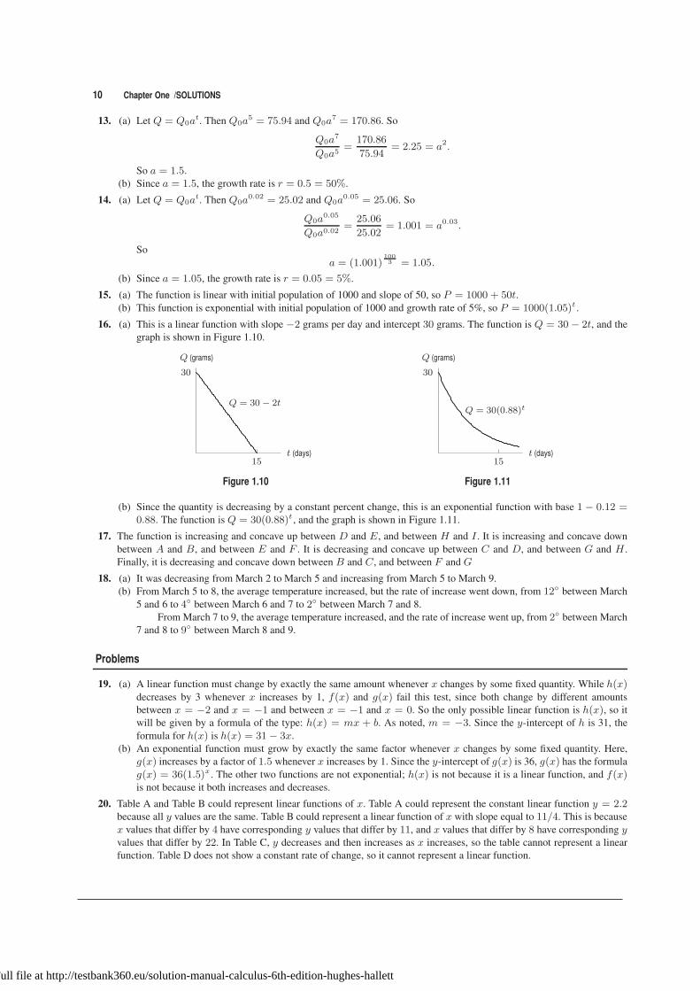
16. (a) This is a linear function with slope −2 grams per day and intercept 30 grams. The function is Q = 30− 2t, and the
graph is shown in Figure 1.10.
30
15
Q (grams)
t (days)
Q = 30 − 2t
Figure 1.10
30
15
Q (grams)
t (days)
Q = 30(0.88)t
Figure 1.11
(b) Since the quantity is decreasing by a constant percent change, this is an exponential function with base 1 − 0.12 =0.88. The function is Q = 30(0.88)t , and the graph is shown in Figure 1.11.
17. The function is increasing and concave up between D and E, and between H and I . It is increasing and concave down
between A and B, and between E and F . It is decreasing and concave up between C and D, and between G and H .
Finally, it is decreasing and concave down between B and C, and between F and G
18. (a) It was decreasing from March 2 to March 5 and increasing from March 5 to March 9.
(b) From March 5 to 8, the average temperature increased, but the rate of increase went down, from 12◦ between March
5 and 6 to 4◦ between March 6 and 7 to 2◦ between March 7 and 8.
From March 7 to 9, the average temperature increased, and the rate of increase went up, from 2◦ between March
7 and 8 to 9◦ between March 8 and 9.
Problems
19. (a) A linear function must change by exactly the same amount whenever x changes by some fixed quantity. While h(x)decreases by 3 whenever x increases by 1, f(x) and g(x) fail this test, since both change by different amounts
between x = −2 and x = −1 and between x = −1 and x = 0. So the only possible linear function is h(x), so it
will be given by a formula of the type: h(x) = mx + b. As noted, m = −3. Since the y-intercept of h is 31, the
formula for h(x) is h(x) = 31− 3x.
(b) An exponential function must grow by exactly the same factor whenever x changes by some fixed quantity. Here,
g(x) increases by a factor of 1.5 whenever x increases by 1. Since the y-intercept of g(x) is 36, g(x) has the formula
g(x) = 36(1.5)x . The other two functions are not exponential; h(x) is not because it is a linear function, and f(x)is not because it both increases and decreases.
20. Table A and Table B could represent linear functions of x. Table A could represent the constant linear function y = 2.2because all y values are the same. Table B could represent a linear function of x with slope equal to 11/4. This is because
x values that differ by 4 have corresponding y values that differ by 11, and x values that differ by 8 have corresponding yvalues that differ by 22. In Table C, y decreases and then increases as x increases, so the table cannot represent a linear
function. Table D does not show a constant rate of change, so it cannot represent a linear function.
Full file at http://testbank360.eu/solution-manual-calculus-6th-edition-hughes-hallett

1.2 SOLUTIONS 11
21. Table D is the only table that could represent an exponential function of x. This is because, in Table D, the ratio of yvalues is the same for all equally spaced x values. Thus, the y values in the table have a constant percent rate of decrease:
9
18=
4.5
9=
2.25
4.5= 0.5.
Table A represents a constant function of x, so it cannot represent an exponential function. In Table B, the ratio between yvalues corresponding to equally spaced x values is not the same. In Table C, y decreases and then increases as x increases.
So neither Table B nor Table C can represent exponential functions.
22. (a) Let P represent the population of the world, and let t represent the number of years since 2010. Then we have
P = 6.91(1.011)t .
(b) According to this formula, the population of the world in the year 2020 (at t = 10) will be P = 6.9(1.011)10 = 7.71billion people.
(c) The graph is shown in Figure 1.12. The population of the world has doubled when P = 13.82; we see on the graph
that this occurs at approximately t = 63.4. Under these assumptions, the doubling time of the world’s population is
about 63.4 years.
63.4
6.91
13.82
t (years)
P (billion people)
Figure 1.12
23. (a) We have P0 = 1 million, and k = 0.02, so P = (1,000,000)(e0.02t).(b)
1,000,000
P
t
24. The doubling time t depends only on the growth rate; it is the solution to
2 = (1.02)t,
since 1.02t represents the factor by which the population has grown after time t. Trial and error shows that (1.02)35 ≈1.9999 and (1.02)36 ≈ 2.0399, so that the doubling time is about 35 years.
25. (a) We have
Reduced size = (0.80) · Original size
or
Original size =1
(0.80)Reduced size = (1.25) Reduced size,
so the copy must be enlarged by a factor of 1.25, which means it is enlarged to 125% of the reduced size.
(b) If a page is copied n times, then
New size = (0.80)n · Original.
We want to solve for n so that
(0.80)n = 0.15.
By trial and error, we find (0.80)8 = 0.168 and (0.80)9 = 0.134. So the page needs to be copied 9 times.
Full file at http://testbank360.eu/solution-manual-calculus-6th-edition-hughes-hallett

12 Chapter One /SOLUTIONS
26. (a) See Figure 1.13.
time
customers
Figure 1.13
(b) “The rate at which new people try it” is the rate of change of the total number of people who have tried the product.
Thus, the statement of the problem is telling you that the graph is concave down—the slope is positive but decreasing,
as the graph shows.
27. (a) Advertising is generally cheaper in bulk; spending more money will give better and better marginal results initially,
(Spending $5,000 could give you a big newspaper ad reaching 200,000 people; spending $100,000 could give you a
series of TV spots reaching 50,000,000 people.) See Figure 1.14.
(b) The temperature of a hot object decreases at a rate proportional to the difference between its temperature and the
temperature of the air around it. Thus, the temperature of a very hot object decreases more quickly than a cooler
object. The graph is decreasing and concave up. See Figure 1.15 (We are assuming that the coffee is all at the same
temperature.)
advertising
revenue
Figure 1.14
time
temperature
Figure 1.15
28. (a) This is the graph of a linear function, which increases at a constant rate, and thus corresponds to k(t), which increases
by 0.3 over each interval of 1.
(b) This graph is concave down, so it corresponds to a function whose increases are getting smaller, as is the case with
h(t), whose increases are 10, 9, 8, 7, and 6.
(c) This graph is concave up, so it corresponds to a function whose increases are getting bigger, as is the case with g(t),whose increases are 1, 2, 3, 4, and 5.
29. (a) This is a linear function, corresponding to g(x), whose rate of decrease is constant, 0.6.
(b) This graph is concave down, so it corresponds to a function whose rate of decrease is increasing, like h(x). (The rates
are −0.2, −0.3, −0.4, −0.5, −0.6.)
(c) This graph is concave up, so it corresponds to a function whose rate of decrease is decreasing, like f(x). (The rates
are −10, −9, −8, −7, −6.)
30. Since we are told that the rate of decay is continuous, we use the function Q(t) = Q0ert to model the decay, where Q(t)
is the amount of strontium-90 which remains at time t, and Q0 is the original amount. Then
Q(t) = Q0e−0.0247t.
So after 100 years,
Q(100) = Q0e−0.0247·100
andQ(100)
Q0= e−2.47 ≈ 0.0846
so about 8.46% of the strontium-90 remains.
Full file at http://testbank360.eu/solution-manual-calculus-6th-edition-hughes-hallett

1.2 SOLUTIONS 13
31. We look for an equation of the form y = y0ax since the graph looks exponential. The points (0, 3) and (2, 12) are on the
graph, so
3 = y0a0 = y0
and
12 = y0 · a2 = 3 · a2, giving a = ±2.
Since a > 0, our equation is y = 3(2x).
32. We look for an equation of the form y = y0ax since the graph looks exponential. The points (−1, 8) and (1, 2) are on the
graph, so
8 = y0a−1 and 2 = y0a
1
Therefore8
2=
y0a−1
y0a=
1
a2, giving a = 1
2, and so 2 = y0a
1 = y0 · 12
, so y0 = 4.
Hence y = 4(
12
)x= 4(2−x).
33. We look for an equation of the form y = y0ax since the graph looks exponential. The points (1, 6) and (2, 18) are on the
graph, so
6 = y0a1
and 18 = y0a2
Therefore a = y0a2
y0a=
18
6= 3, and so 6 = y0a = y0 · 3; thus, y0 = 2. Hence y = 2(3x).
34. The difference, D, between the horizontal asymptote and the graph appears to decrease exponentially, so we look for an
equation of the form
D = D0ax
where D0 = 4 = difference when x = 0. Since D = 4− y, we have
4− y = 4axor y = 4− 4ax = 4(1− ax)
The point (1, 2) is on the graph, so 2 = 4(1− a1), giving a = 12.
Therefore y = 4(1− ( 12)x) = 4(1− 2−x).
35. Since f is linear, its slope is a constant
m =20− 10
2− 0= 5.
Thus f increases 5 units for unit increase in x, so
f(1) = 15, f(3) = 25, f(4) = 30.
Since g is exponential, its growth factor is constant. Writing g(x) = abx, we have g(0) = a = 10, so
g(x) = 10 · bx.
Since g(2) = 10 · b2 = 20, we have b2 = 2 and since b > 0, we have
b =√2.
Thus g increases by a factor of√2 for unit increase in x, so
g(1) = 10√2, g(3) = 10(
√2)3 = 20
√2, g(4) = 10(
√2)4 = 40.
Notice that the value of g(x) doubles between x = 0 and x = 2 (from g(0) = 10 to g(2) = 20), so the doubling time of
g(x) is 2. Thus, g(x) doubles again between x = 2 and x = 4, confirming that g(4) = 40.
36. We see that 1.091.06
≈ 1.03, and therefore h(s) = c(1.03)s; c must be 1. Similarly 2.422.20
= 1.1, and so f(s) = a(1.1)s;
a = 2. Lastly, 3.653.47
≈ 1.05, so g(s) = b(1.05)s; b ≈ 3.
37. (a) Because the population is growing exponentially, the time it takes to double is the same, regardless of the population
levels we are considering. For example, the population is 20,000 at time 3.7, and 40,000 at time 6.0. This represents
a doubling of the population in a span of 6.0− 3.7 = 2.3 years.
How long does it take the population to double a second time, from 40,000 to 80,000? Looking at the graph once
again, we see that the population reaches 80,000 at time t = 8.3. This second doubling has taken 8.3 − 6.0 = 2.3years, the same amount of time as the first doubling.
Further comparison of any two populations on this graph that differ by a factor of two will show that the time
that separates them is 2.3 years. Similarly, during any 2.3 year period, the population will double. Thus, the doubling
time is 2.3 years.
(b) Suppose P = P0at doubles from time t to time t + d. We now have P0a
t+d = 2P0at, so P0a
tad = 2P0at. Thus,
canceling P0 and at, d must be the number such that ad = 2, no matter what t is.
Full file at http://testbank360.eu/solution-manual-calculus-6th-edition-hughes-hallett

14 Chapter One /SOLUTIONS
38. (a) After 50 years, the amount of money is
P = 2P0.
After 100 years, the amount of money is
P = 2(2P0) = 4P0.
After 150 years, the amount of money is
P = 2(4P0) = 8P0.
(b) The amount of money in the account doubles every 50 years. Thus in t years, the balance doubles t/50 times, so
P = P02t/50.
39. (a) Since 162.5 = 325/2, there are 162.5 mg remaining after H hours.
Since 81.25 = 162.5/2, there are 81.25 mg remaining H hours after there were 162.5 mg, so 2H hours after there
were 325 mg.
Since 40.625 = 81.25/2, there are 41.625 mg remaining H hours after there were 81.25 mg, so 3H hours after there
were 325 mg.
(b) Each additional H hours, the quantity is halved. Thus in t hours, the quantity was halved t/H times, so
A = 325(
1
2
)t/H
.
40. (a) The quantity of radium decays exponentially, so we know Q = Q0at. When t = 1620, we have Q = Q0/2 so
Q0
2= Q0a
1620.
Thus, canceling Q0, we have
a1620 =1
2
a =(
1
2
)1/1620
.
Thus the formula is Q = Q0
(
(
12
)1/1620)t
= Q0
(
12
)t/1620.
(b) After 500 years,
Fraction remaining =1
Q0·Q0
(
1
2
)500/1620
= 0.80740.
so 80.740% is left.
41. Let Q0 be the initial quantity absorbed in 1960. Then the quantity, Q, of strontium-90 left after t years is
Q = Q0
(
1
2
)t/29
.
Since 2010 − 1960 = 50 years, in 2010
Fraction remaining =1
Q0·Q0
(
1
2
)50/29
=(
1
2
)50/29
= 0.30268 = 30.268%.
42. Direct calculation reveals that each 1000 foot increase in altitude results in a longer takeoff roll by a factor of about 1.096.
Since the value of d when h = 0 (sea level) is d = 670, we are led to the formula
d = 670(1.096)h/1000 ,
where d is the takeoff roll, in feet, and h is the airport’s elevation, in feet.
Alternatively, we can write
d = d0ah,
where d0 is the sea level value of d, d0 = 670. In addition, when h = 1000, d = 734, so
734 = 670a1000 .
Solving for a gives
a =(
734
670
)1/1000
= 1.00009124,
so
d = 670(1.00009124)h .
Full file at http://testbank360.eu/solution-manual-calculus-6th-edition-hughes-hallett

1.2 SOLUTIONS 15
43. (a) Since the annual growth factor from 2005 to 2006 was 1 + 1.866 = 2.866 and 91(1 + 1.866) = 260.806, the US
consumed approximately 261 million gallons of biodiesel in 2006. Since the annual growth factor from 2006 to 2007was 1+ 0.372 = 1.372 and 261(1 + 0.372) = 358.092, the US consumed about 358 million gallons of biodiesel in
2007.
(b) Completing the table of annual consumption of biodiesel and plotting the data gives Figure 1.16.
Year 2005 2006 2007 2008 2009
Consumption of biodiesel (mn gal) 91 261 358 316 339
2006 2008
200
400
year
consumption ofbiodiesel (mn gal)
Figure 1.16
44. (a) False, because the annual percent growth is not constant over this interval.
(b) The US consumption of biodiesel more than doubled in 2005 and more than doubled again in 2006. This is because
the annual percent growth was larger than 100% for both of these years.
(c) The US consumption of biodiesel more than tripled in 2005, since the annual percent growth in 2005 was over 200%
45. (a) Since the annual growth factor from 2006 to 2007 was 1 − 0.454 = 0.546 and 29(1 − 0.454) = 15.834, the US
consumed approximately 16 trillion BTUs of hydroelectric power in 2007. Since the annual growth factor from 2005
to 2006 was 1 − 0.10 = 0.90 and29
(1− 0.10)= 32.222, the US consumed about 32 trillion BTUs of hydroelectric
power in 2005.
(b) Completing the table of annual consumption of hydroelectric power and plotting the data gives Figure 1.17.
Year 2004 2005 2006 2007 2008 2009
Consumption of hydro. power (trillion BTU) 33 32 29 16 17 19
(c) The largest decrease in the US consumption of hydroelectric power occurred in 2007. In this year, the US consump-
tion of hydroelectric power dropped by about 13 trillion BTUs to 16 trillion BTUs, down from 29 trillion BTUs in
2006.
2005 2007 2009
5
15
25
35
year
consumption of hydro.power (trillion BTU)
Figure 1.17
Full file at http://testbank360.eu/solution-manual-calculus-6th-edition-hughes-hallett

16 Chapter One /SOLUTIONS
46. (a) From the figure we can read-off the approximate percent growth for each year over the previous year:
Year 2005 2006 2007 2008 2009
% growth over previous yr 25 50 30 60 29
Since the annual growth factor from 2006 to 2007 was 1 + 0.30 = 1.30 and
341
(1 + 0.30)= 262.31,
the US consumed approximately 262 trillion BTUs of wind power energy in 2006. Since the annual growth factor
from 2007 to 2008 was 1 + 0.60 = 1.60 and 341(1 + 0.60) = 545.6, the US consumed about 546 trillion BTUs of
wind power energy in 2008.
(b) Completing the table of annual consumption of wind power and plotting the data gives Figure 1.18.
Year 2005 2006 2007 2008 2009
Consumption of wind power (trillion BTU) 175 262 341 546 704
(c) The largest increase in the US consumption of wind power energy occurred in 2008. In this year the US consumption
of wind power energy rose by about 205 trillion BTUs to 546 trillion BTUs, up from 341 trillion BTUs in 2007.
2007 2009
100
300
500
700
year
consumption of wind powerenergy (trillion BTU)
Figure 1.18
47. (a) The US consumption of wind power energy increased by at least 40% in 2006 and in 2008, relative to the previ-
ous year. In 2006 consumption increased by just under 50% over consumption in 2005, and in 2008 consumption
increased by about 60% over consumption in 2007. Consumption did not decrease during the time period shown
because all the annual percent growth values are positive, indicating a steady increase in the US consumption of wind
power energy between 2005 and 2009.
(b) Yes. From 2006 to 2007 consumption increased by about 30%, which means x(1+0.30) units of wind power energy
were consumed in 2007 if x had been consumed in 2006. Similarly,
(x(1 + 0.30))(1 + 0.60)
units of wind power energy were consumed in 2008 if x had been consumed in 2006 (because consumption increased
by about 60% from 2007 to 2008). Since
(x(1 + 0.30))(1 + 0.60) = x(2.08) = x(1 + 1.08),
the percent growth in wind power consumption was about 108%, or just over 100%, in 2008 relative to consumption
in 2006.
Strengthen Your Understanding
48. The function y = e−0.25x is decreasing but its graph is concave up.
49. The graph of y = 2x is a straight line and is neither concave up or concave down.
Full file at http://testbank360.eu/solution-manual-calculus-6th-edition-hughes-hallett

1.3 SOLUTIONS 17
50. One possible answer is q = 2.2(0.97)t .
51. One possible answer is f(x) = 2(1.1)x.
52. One possibility is y = e−x − 5.
53. False. The y-intercept is y = 2 + 3e−0 = 5.
54. True, since, as t → ∞, we know e−4t → 0, so y = 5− 3e−4t → 5.
55. False. Suppose y = 5x. Then increasing x by 1 increases y by a factor of 5. However increasing x by 2 increases y by a
factor of 25, not 10, since
y = 5x+2 = 5x · 52 = 25 · 5x.(Other examples are possible.)
56. True. Suppose y = Abx and we start at the point (x1, y1), so y1 = Abx1 . Then increasing x1 by 1 gives x1 + 1, so the
new y-value, y2, is given by
y2 = Abx1+1 = Abx1b = (Abx1)b,
so
y2 = by1.
Thus, y has increased by a factor of b, so b = 3, and the function is y = A3x.
However, if x1 is increased by 2, giving x1 + 2, then the new y-value, y3, is given by
y3 = A3x1+2 = A3x132 = 9A3x1 = 9y1.
Thus, y has increased by a factor of 9.
57. True. For example, f(x) = (0.5)x is an exponential function which decreases. (Other examples are possible.)
58. True. If b > 1, then abx → 0 as x → −∞. If 0 < b < 1, then abx → 0 as x → ∞. In either case, the function
y = a+ abx has y = a as the horizontal asymptote.
59. True, since e−kt → 0 as t → ∞, so y → 20 as t → ∞.
Solutions for Section 1.3
Exercises
1.
−2 2
−4
4
x
y(a)
−2 2
−4
4
x
y(b)
−2 2
−4
4
x
y(c)
−2 2
−4
4
x
y(d)
−2 2
−4
4
x
y(e)
−2 2
−4
4
x
y(f)
Full file at http://testbank360.eu/solution-manual-calculus-6th-edition-hughes-hallett

18 Chapter One /SOLUTIONS
2.
−2 2
−4
4
x
y(a)
−2 2
−4
4
x
y(b)
−2 2
−4
4
x
y(c)
−2 2
−4
4
x
y(d)
−2 2
−4
4
x
y(e)
−2 2
−4
4
x
y(f)
3.
−2 2
−4
4
x
y(a)
−2 2
−4
4
x
y(b)
−2 2
−4
4
x
y(c)
−2 2
−4
4
x
y(d)
−2 2
−4
4
x
y(e)
−2 2
−4
4
x
y(f)
Full file at http://testbank360.eu/solution-manual-calculus-6th-edition-hughes-hallett

1.3 SOLUTIONS 19
4. This graph is the graph of m(t) shifted upward by two units. See Figure 1.19.
−4 4 6
−4
4
n(t)
t
Figure 1.19
5. This graph is the graph of m(t) shifted to the right by one unit. See Figure 1.20.
−4 4 6
−4
4
p(t)
t
y
Figure 1.20
6. This graph is the graph of m(t) shifted to the left by 1.5 units. See Figure 1.21.
−4
4 6
−4
4
k(t)
t
Figure 1.21
7. This graph is the graph of m(t) shifted to the right by 0.5 units and downward by 2.5 units. See Figure 1.22.
−4 6
−4
4
w(t)
t
Figure 1.22
Full file at http://testbank360.eu/solution-manual-calculus-6th-edition-hughes-hallett

20 Chapter One /SOLUTIONS
8. (a) f(g(1)) = f(1 + 1) = f(2) = 22 = 4(b) g(f(1)) = g(12) = g(1) = 1 + 1 = 2(c) f(g(x)) = f(x+ 1) = (x+ 1)2
(d) g(f(x)) = g(x2) = x2 + 1(e) f(t)g(t) = t2(t+ 1)
9. (a) f(g(1)) = f(12) = f(1) =√1 + 4 =
√5
(b) g(f(1)) = g(√1 + 4) = g(
√5) = (
√5)2 = 5
(c) f(g(x)) = f(x2) =√x2 + 4
(d) g(f(x)) = g(√x+ 4) = (
√x+ 4)2 = x+ 4
(e) f(t)g(t) = (√t+ 4)t2 = t2
√t+ 4
10. (a) f(g(1)) = f(12) = f(1) = e1 = e(b) g(f(1)) = g(e1) = g(e) = e2
(c) f(g(x)) = f(x2) = ex2
(d) g(f(x)) = g(ex) = (ex)2 = e2x
(e) f(t)g(t) = ett2
11. (a) f(g(1)) = f(3 · 1 + 4) = f(7) =1
7(b) g(f(1)) = g(1/1) = g(1) = 7
(c) f(g(x)) = f(3x + 4) =1
3x+ 4
(d) g(f(x)) = g(
1
x
)
= 3(
1
x
)
+ 4 =3
x+ 4
(e) f(t)g(t) =1
t(3t+ 4) = 3 +
4
t
12. (a) g(2 + h) = (2 + h)2 + 2(2 + h) + 3 = 4 + 4h+ h2 + 4 + 2h+ 3 = h2 + 6h+ 11.
(b) g(2) = 22 + 2(2) + 3 = 4 + 4 + 3 = 11, which agrees with what we get by substituting h = 0 into (a).
(c) g(2 + h)− g(2) = (h2 + 6h+ 11)− (11) = h2 + 6h.
13. (a) f(t+ 1) = (t+ 1)2 + 1 = t2 + 2t+ 1 + 1 = t2 + 2t+ 2.
(b) f(t2 + 1) = (t2 + 1)2 + 1 = t4 + 2t2 + 1 + 1 = t4 + 2t2 + 2.
(c) f(2) = 22 + 1 = 5.
(d) 2f(t) = 2(t2 + 1) = 2t2 + 2.
(e) (f(t))2 + 1 =(
t2 + 1)2
+ 1 = t4 + 2t2 + 1 + 1 = t4 + 2t2 + 2.
14. m(z + 1)−m(z) = (z + 1)2 − z2 = 2z + 1.
15. m(z + h)−m(z) = (z + h)2 − z2 = 2zh+ h2.
16. m(z)−m(z − h) = z2 − (z − h)2 = 2zh− h2.
17. m(z + h)−m(z − h) = (z + h)2 − (z − h)2 = z2 + 2hz + h2 − (z2 − 2hz + h2) = 4hz.
18. (a) f(25) is q corresponding to p = 25, or, in other words, the number of items sold when the price is 25.
(b) f−1(30) is p corresponding to q = 30, or the price at which 30 units will be sold.
19. (a) f(10,000) represents the value of C corresponding to A = 10,000, or in other words the cost of building a 10,000square-foot store.
(b) f−1(20,000) represents the value of A corresponding to C = 20,000, or the area in square feet of a store which
would cost $20,000 to build.
20. f−1(75) is the length of the column of mercury in the thermometer when the temperature is 75◦F.
21. (a) The equation is y = 2x2 + 1. Note that its graph is narrower than the graph of y = x2 which appears in gray. See
Figure 1.23.
2
4
6
8 y = 2x2 + 1
y = x2
Figure 1.23
12
34
56
7
8 y = 2(x2 + 1)
y = x2
Figure 1.24
Full file at http://testbank360.eu/solution-manual-calculus-6th-edition-hughes-hallett

1.3 SOLUTIONS 21
(b) y = 2(x2 + 1) moves the graph up one unit and then stretches it by a factor of two. See Figure 1.24.
(c) No, the graphs are not the same. Since 2(x2 + 1) = (2x2 + 1) + 1, the second graph is always one unit higher than
the first.
22. Figure 1.25 shows the appropriate graphs. Note that asymptotes are shown as dashed lines and x- or y-intercepts are
shown as filled circles.
−5 5−3 2
2
5
x
y
y = 3
(a)
−5 −3 2 5
−2
2
4
x
y(b)
−10 −6 2−1
1
2
5
x
y(c)
−5 −1 2 5
2
5
x
y
y = 4
(d)
Figure 1.25
23. The function is not invertible since there are many horizontal lines which hit the function twice.
24. The function is not invertible since there are horizontal lines which hit the function more than once.
25. Since a horizontal line cuts the graph of f(x) = x2 + 3x+ 2 two times, f is not invertible. See Figure 1.26.
32
−3
4
y = 2.5
f(x) = x2 + 3x+ 2
x
y
Figure 1.26
Full file at http://testbank360.eu/solution-manual-calculus-6th-edition-hughes-hallett

22 Chapter One /SOLUTIONS
26. Since a horizontal line cuts the graph of f(x) = x3 − 5x+ 10 three times, f is not invertible. See Figure 1.27.
x
y
-2 2
y = 8
10
f(x) = x3 − 5x+ 10
Figure 1.27
27. Since any horizontal line cuts the graph once, f is invertible. See Figure 1.28.
x
y
-2 2
20
40
y = 30
f(x) = x3 + 5x+ 10
y = −19
Figure 1.28
28.
f(−x) = (−x)6 + (−x)3 + 1 = x6 − x3 + 1.
Since f(−x) 6= f(x) and f(−x) 6= −f(x), this function is neither even nor odd.
29.
f(−x) = (−x)3 + (−x)2 + (−x) = −x3 + x2 − x.
Since f(−x) 6= f(x) and f(−x) 6= −f(x), this function is neither even nor odd.
30. Since
f(−x) = (−x)4 − (−x)2 + 3 = x4 − x2 + 3 = f(x),
we see f is even
31. Since
f(−x) = (−x)3 + 1 = −x3 + 1,
we see f(−x) 6= f(x) and f(−x) 6= −f(x), so f is neither even nor odd
32. Since
f(−x) = 2(−x) = −2x = −f(x),
we see f is odd.
Full file at http://testbank360.eu/solution-manual-calculus-6th-edition-hughes-hallett

1.3 SOLUTIONS 23
33. Since
f(−x) = e(−x)2−1 = ex2−1 = f(x),
we see f is even.
34. Since
f(−x) = (−x)((−x)2 − 1) = −x(x2 − 1) = −f(x),
we see f is odd
35. Since
f(−x) = e−x + x,
we see f(−x) 6= f(x) and f(−x) 6= −f(x), so f is neither even nor odd
Problems
36. f(x) = x3, g(x) = x+ 1.
37. f(x) = x+ 1, g(x) = x3.
38. f(x) =√x, g(x) = x2 + 4
39. f(x) = ex, g(x) = 2x
40. This looks like a shift of the graph y = −x2. The graph is shifted to the left 1 unit and up 3 units, so a possible formula
is y = −(x+ 1)2 + 3.
41. This looks like a shift of the graph y = x3. The graph is shifted to the right 2 units and down 1 unit, so a possible formula
is y = (x− 2)3 − 1.
42. (a) We find f−1(2) by finding the x value corresponding to f(x) = 2. Looking at the graph, we see that f−1(2) = −1.
(b) We construct the graph of f−1(x) by reflecting the graph of f(x) over the line y = x. The graphs of f−1(x) and
f(x) are shown together in Figure 1.29.
−4 6
−4
4
x
y
f−1(x)
f(x)
Figure 1.29
43. Values of f−1 are as follows
x 3 −7 19 4 178 2 1
f−1(x) 1 2 3 4 5 6 7
The domain of f−1 is the set consisting of the integers {3,−7, 19, 4, 178, 2, 1}.
44. f is an increasing function since the amount of fuel used increases as flight time increases. Therefore f is invertible.
45. Not invertible. Given a certain number of customers, say f(t) = 1500, there could be many times, t, during the day at
which that many people were in the store. So we don’t know which time instant is the right one.
46. Probably not invertible. Since your calculus class probably has less than 363 students, there will be at least two days in
the year, say a and b, with f(a) = f(b) = 0. Hence we don’t know what to choose for f−1(0).
47. Not invertible, since it costs the same to mail a 50-gram letter as it does to mail a 51-gram letter.
48. The volume of the balloon t minutes after inflation began is: g(f(t)) ft3.
49. The volume of the balloon if its radius were twice as big is: g(2r) ft3.
Full file at http://testbank360.eu/solution-manual-calculus-6th-edition-hughes-hallett

24 Chapter One /SOLUTIONS
50. The time elapsed is: f−1(30) min.
51. The time elapsed is: f−1(g−1(10,000)) min.
52. We have v(10) = 65 but the graph of u only enables us to evaluate u(x) for 0 ≤ x ≤ 50. There is not enough information
to evaluate u(v(10)).
53. We have approximately v(40) = 15 and u(15) = 18 so u(v(40)) = 18.
54. We have approximately u(10) = 13 and v(13) = 60 so v(u(10)) = 60.
55. We have u(40) = 60 but the graph of v only enables us to evaluate v(x) for 0 ≤ x ≤ 50. There is not enough information
to evaluate v(u(40)).
56. (a) Yes, f is invertible, since f is increasing everywhere.
(b) The number f−1(400) is the year in which 400 million motor vehicles were registered in the world. From the picture,
we see that f−1(400) is around 1979.
(c) Since the graph of f−1 is the reflection of the graph of f over the line y = x, we get Figure 1.30.
200 400 600 800 1000’65’70’75’80’85’90’95’00’05’10
(millions)
(year)
Figure 1.30: Graph of f−1
57. f(g(1)) = f(2) ≈ 0.4.
58. g(f(2)) ≈ g(0.4) ≈ 1.1.
59. f(f(1)) ≈ f(−0.4) ≈ −0.9.
60. Computing f(g(x)) as in Problem 57, we get Table 1.2. From it we graph f(g(x)) in Figure 1.31.
Table 1.2
x g(x) f(g(x))
−3 0.6 −0.5
−2.5 −1.1 −1.3
−2 −1.9 −1.2
−1.5 −1.9 −1.2
−1 −1.4 −1.3
−0.5 −0.5 −1
0 0.5 −0.6
0.5 1.4 −0.2
1 2 0.4
1.5 2.2 0.5
2 1.6 0
2.5 0.1 −0.7
3 −2.5 0.1
−3 3
−3
3
xf(g(x))
Figure 1.31
61. Using the same way to compute g(f(x)) as in Problem 58, we get Table 1.3. Then we can plot the graph of g(f(x)) in
Figure 1.32.
Full file at http://testbank360.eu/solution-manual-calculus-6th-edition-hughes-hallett

1.3 SOLUTIONS 25
Table 1.3
x f(x) g(f(x))
−3 3 −2.6
−2.5 0.1 0.8
−2 −1 −1.4
−1.5 −1.3 −1.8
−1 −1.2 −1.7
−0.5 −1 −1.4
0 −0.8 −1
0.5 −0.6 −0.6
1 −0.4 −0.3
1.5 −0.1 0.3
2 0.3 1.1
2.5 0.9 2
3 1.6 2.2
−3 3
−3
3
x
g(f(x))
Figure 1.32
62. Using the same way to compute f(f(x)) as in Problem 59, we get Table 1.4. Then we can plot the graph of f(f(x)) in
Figure 1.33.
Table 1.4
x f(x) f(f(x))
−3 3 1.6
−2.5 0.1 −0.7
−2 −1 −1.2
−1.5 −1.3 −1.3
−1 −1.2 −1.3
−0.5 −1 −1.2
0 −0.8 −1.1
0.5 −0.6 −1
1 −0.4 −0.9
1.5 −0.1 −0.8
2 0.3 −0.6
2.5 0.9 −0.4
3 1.6 0
−3 3
−3
3
x
f(f(x))
Figure 1.33
63. (a) The graph shows that f(15) is approximately 48. So, the place to find find 15 million-year-old rock is about 48meters below the Atlantic sea floor.
(b) Since f is increasing (not decreasing, since the depth axis is reversed!), f is invertible. To confirm, notice that the
graph of f is cut by a horizontal line at most once.
(c) Look at where the horizontal line through 120 intersects the graph of f and read downward: f−1(120) is about 35.
In practical terms, this means that at a depth of 120 meters down, the rock is 35 million years old.
(d) First, we standardize the graph of f so that time and depth are increasing from left to right and bottom to top. Points
(t, d) on the graph of f correspond to points (d, t) on the graph of f−1. We can graph f−1 by taking points from
the original graph of f , reversing their coordinates, and connecting them. This amounts to interchanging the t and daxes, thereby reflecting the graph of f about the line bisecting the 90◦ angle at the origin. Figure 1.34 is the graph of
f−1. (Note that we cannot find the graph of f−1 by flipping the graph of f about the line t = d in because t and dhave different scales in this instance.)
Full file at http://testbank360.eu/solution-manual-calculus-6th-edition-hughes-hallett

26 Chapter One /SOLUTIONS
✒
✠
✒
✠
f−1
f (standardized)
30Time10
20
Depth
100
10020 Depth
Time
10
30
Figure 1.34: Graph of f , reflected to give that of f−1
64. The tree has B = y − 1 branches on average and each branch has n = 2B2 − B = 2(y − 1)2 − (y − 1) leaves on
average. Therefore
Average number of leaves = Bn = (y − 1)(2(y − 1)2 − (y − 1)) = 2(y − 1)3 − (y − 1)2.
65. The volume, V , of the balloon is V = 43πr3. When t = 3, the radius is 10 cm. The volume is then
V =4
3π(103) =
4000π
3cm
3.
66. (a) The function f tells us C in terms of q. To get its inverse, we want q in terms of C, which we find by solving for q:
C = 100 + 2q,
C − 100 = 2q,
q =C − 100
2= f−1(C).
(b) The inverse function tells us the number of articles that can be produced for a given cost.
67. Since Q = S − Se−kt, the graph of Q is the reflection of y about the t-axis moved up by S units.
68.x f(x) g(x) h(x)
−3 0 0 0
−2 2 2 −2
−1 2 2 −2
0 0 0 0
1 2 −2 −2
2 2 −2 −2
3 0 0 0
Strengthen Your Understanding
69. The graph of f(x) = −(x+ 1)3 is the graph of g(x) = −x3 shifted left by 1 unit.
70. Since f(g(x)) = 3(−3x− 5) + 5 = −9x− 10, we see that f and g are not inverse functions.
71. While y = 1/x is sometimes referred to as the multiplicative inverse of x, the inverse of f is f−1(x) = x.
72. One possible answer is g(x) = 3 + x. (There are many answers.)
73. One possibility is f(x) = x2 + 2.
74. Let f(x) = 3x, then f−1(x) = x/3. Then for x > 0, we have f(x) > f−1(x).
Full file at http://testbank360.eu/solution-manual-calculus-6th-edition-hughes-hallett

1.4 SOLUTIONS 27
75. We have
g(x) = f(x+ 2)
because the graph of g is obtained by moving the graph of f to the left by 2 units. We also have
g(x) = f(x) + 3
because the graph of g is obtained by moving the graph of f up by 3 units. Thus, we have f(x+2) = f(x)+3. The graph
of f climbs 3 units whenever x increases by 2. The simplest choice for f is a linear function of slope 3/2, for example
f(x) = 1.5x, so g(x) = 1.5x + 3.
76. True. The graph of y = 10x is moved horizontally by h units if we replace x by x − h for some number h. Writing
100 = 102, we have f(x) = 100(10x) = 102 · 10x = 10x+2. The graph of f(x) = 10x+2 is the graph of g(x) = 10x
shifted two units to the left.
77. True. If f is increasing then its reflection about the line y = x is also increasing. An example is shown in Figure 1.35.
The statement is true.
−4 6
−4
4
f(x)
x = y
f−1(x)
x
y
Figure 1.35
78. True. If f(x) is even, we have f(x) = f(−x) for all x. For example, f(−2) = f(2). This means that the graph of f(x)intersects the horizontal line y = f(2) at two points, x = 2 and x = −2. Thus, f has no inverse function.
79. False. For example, f(x) = x and g(x) = x3 are both odd. Their inverses are f−1(x) = x and g−1(x) = x1/3.
80. False. For x < 0, as x increases, x2 decreases, so e−x2
increases.
81. True. We have g(−x) = g(x) since g is even, and therefore f(g(−x)) = f(g(x)).
82. False. A counterexample is given by f(x) = x2 and g(x) = x+1. The function f(g(x)) = (x+1)2 is not even because
f(g(1)) = 4 and f(g(−1)) = 0 6= 4.
83. True. The constant function f(x) = 0 is the only function that is both even and odd. This follows, since if f is both even
and odd, then, for all x, f(−x) = f(x) (if f is even) and f(−x) = −f(x) (if f is odd). Thus, for all x, f(x) = −f(x)i.e. f(x) = 0, for all x. So f(x) = 0 is both even and odd and is the only such function.
84. Let f(x) = x and g(x) = −2x. Then f(x) + g(x) = −x, which is decreasing. Note f is increasing since it has positive
slope, and g is decreasing since it has negative slope.
85. This is impossible. If a < b, then f(a) < f(b), since f is increasing, and g(a) > g(b), since g is decreasing, so
−g(a) < −g(b). Therefore, if a < b, then f(a)− g(a) < f(b)− g(b), which means that f(x) + g(x) is increasing.
86. Let f(x) = ex and let g(x) = e−2x. Note f is increasing since it is an exponential growth function, and g is decreasing
since it is an exponential decay function. Then f(x)g(x) = e−x, which is decreasing.
87. This is impossible. As x increases, g(x) decreases. As g(x) decreases, so does f(g(x)) because f is increasing (an
increasing function increases as its variable increases, so it decreases as its variable decreases).
Solutions for Section 1.4
Exercises
1. Using the identity elnx = x, we have eln(1/2) = 12
.
Full file at http://testbank360.eu/solution-manual-calculus-6th-edition-hughes-hallett

28 Chapter One /SOLUTIONS
2. Using the identity 10log x = x, we have
10log(AB) = AB
3. Using the identity elnx = x, we have 5A2.
4. Using the identity ln (ex) = x, we have 2AB.
5. Using the rules for ln, we have
ln(
1
e
)
+ lnAB = ln 1− ln e+ lnA+ lnB
= 0− 1 + lnA+ lnB
= −1 + lnA+ lnB.
6. Using the rules for ln, we have 2A+ 3e lnB.
7. Taking logs of both sides
log 3x = x log 3 = log 11
x =log 11
log 3= 2.2.
8. Taking logs of both sides
log 17x = log 2
x log 17 = log 2
x =log 2
log 17≈ 0.24.
9. Isolating the exponential term
20 = 50(1.04)x
20
50= (1.04)x.
Taking logs of both sides
log2
5= log(1.04)x
log2
5= x log(1.04)
x =log(2/5)
log(1.04)= −23.4.
10.
4
7=
5x
3x
4
7=(
5
3
)x
Taking logs of both sides
log(
4
7
)
= x log(
5
3
)
x =log(4/7)
log(5/3)≈ −1.1.
Full file at http://testbank360.eu/solution-manual-calculus-6th-edition-hughes-hallett

1.4 SOLUTIONS 29
11. To solve for x, we first divide both sides by 5 and then take the natural logarithm of both sides.
7
5= e0.2x
ln(7/5) = 0.2x
x =ln(7/5)
0.2≈ 1.68.
12. ln(2x) = ln(ex+1)
x ln 2 = (x+ 1) ln e
x ln 2 = x+ 1
0.693x = x+ 1
x =1
0.693 − 1≈ −3.26
13. To solve for x, we first divide both sides by 600 and then take the natural logarithm of both sides.
50
600= e−0.4x
ln(50/600) = −0.4x
x =ln(50/600)
−0.4≈ 6.212.
14. ln(2e3x) = ln(4e5x)
ln 2 + ln(e3x) = ln 4 + ln(e5x)
0.693 + 3x = 1.386 + 5x
x = −0.347
15. Using the rules for ln, we get
ln 7x+2 = ln e17x
(x+ 2) ln 7 = 17x
x(ln 7− 17) = −2 ln 7
x =−2 ln 7
ln 7− 17≈ 0.26.
16. ln(10x+3) = ln(5e7−x)
(x+ 3) ln 10 = ln 5 + (7− x) ln e
2.303(x + 3) = 1.609 + (7− x)
3.303x = 1.609 + 7− 2.303(3)
x = 0.515
17. Using the rules for ln, we have
2x− 1 = x2
x2 − 2x+ 1 = 0
(x− 1)2 = 0
x = 1.
18. 4e2x−3 = e+ 5
ln 4 + ln(e2x−3) = ln(e+ 5)
1.3863 + 2x− 3 = 2.0436
x = 1.839.
19. t =log a
log b.
Full file at http://testbank360.eu/solution-manual-calculus-6th-edition-hughes-hallett

30 Chapter One /SOLUTIONS
20. t =log
(
PP0
)
log a=
logP − logP0
log a.
21. Taking logs of both sides yields
nt =log
(
QQ0
)
log a.
Hence
t =log
(
QQ0
)
n log a=
logQ− logQ0
n log a.
22. Collecting similar terms yields(
a
b
)t
=Q0
P0.
Hence
t =log
(
Q0
P0
)
log(
ab
) .
23. t = lna
b.
24. lnP
P0= kt, so t =
ln PP0
k.
25. Since we want (1.5)t = ekt = (ek)t, so 1.5 = ek, and k = ln 1.5 = 0.4055. Thus, P = 15e0.4055t . Since 0.4055 is
positive, this is exponential growth.
26. We want 1.7t = ekt so 1.7 = ek and k = ln 1.7 = 0.5306. Thus P = 10e0.5306t .
27. We want 0.9t = ekt so 0.9 = ek and k = ln 0.9 = −0.1054. Thus P = 174e−0.1054t .
28. Since we want (0.55)t = ekt = (ek)t, so 0.55 = ek, and k = ln 0.55 = −0.5978. Thus P = 4e−0.5978t . Since
−0.5978 is negative, this represents exponential decay.
29. If p(t) = (1.04)t, then, for p−1 the inverse of p, we should have
(1.04)p−1(t) = t,
p−1(t) log(1.04) = log t,
p−1(t) =log t
log(1.04)≈ 58.708 log t.
30. Since f is increasing, f has an inverse. To find the inverse of f(t) = 50e0.1t, we replace t with f−1(t), and, since
f(f−1(t)) = t, we have
t = 50e0.1f−1(t).
We then solve for f−1(t):
t = 50e0.1f−1(t)
t
50= e0.1f
−1(t)
ln(
t
50
)
= 0.1f−1(t)
f−1(t) =1
0.1ln(
t
50
)
= 10 ln(
t
50
)
.
31. Using f(f−1(t)) = t, we see
f(f−1(t)) = 1 + ln f−1(t) = t.
So
ln f−1(t) = t− 1
f−1(t) = et−1.
Full file at http://testbank360.eu/solution-manual-calculus-6th-edition-hughes-hallett

1.4 SOLUTIONS 31
Problems
32. The population has increased by a factor of 48,000,000/40,000,000 = 1.2 in 10 years. Thus we have the formula
P = 40,000,000(1.2)t/10 ,
and t/10 gives the number of 10-year periods that have passed since 2000.
In 2000, t/10 = 0, so we have P = 40,000,000.
In 2010, t/10 = 1, so P = 40,000,000(1.2) = 48,000,000.
In 2020, t/10 = 2, so P = 40,000,000(1.2)2 = 57,600,000.
To find the doubling time, solve 80,000,000 = 40,000,000(1.2)t/10 , to get t = 38.02 years.
33. In ten years, the substance has decayed to 40% of its original mass. In another ten years, it will decay by an additional
factor of 40%, so the amount remaining after 20 years will be 100 · 40% · 40% = 16 kg.
34. We can solve for the growth rate k of the bacteria using the formula P = P0ekt:
1500 = 500ek(2)
k =ln(1500/500)
2.
Knowing the growth rate, we can find the population P at time t = 6:
P = 500e(ln 32
)6
≈ 13,500 bacteria.
35. (a) Assuming the US population grows exponentially, we have population P (t) = 281.4ekt at time t years after 2000.
Using the 2010 population, we have
308.7 = 281.4e10k
k =ln(308.7/281.4)
10= 0.00926.
We want to find the time t in which
350 = 281.4e0.00926t
t =ln(350/281.4)
0.00926= 23.56 years.
This model predicts the population to go over 350 million 23.56 years after 2000, in the year 2023.
(b) Evaluate P = 281.4e0.00926t for t = 20 to find P = 338.65 million people.
36. If C0 is the concentration of NO2 on the road, then the concentration x meters from the road is
C = C0e−0.0254x.
We want to find the value of x making C = C0/2, that is,
C0e−0.0254x =
C0
2.
Dividing by C0 and then taking natural logs yields
ln(
e−0.254x)
= −0.0254x = ln(
1
2
)
= −0.6931,
so
x = 27 meters.
At 27 meters from the road the concentration of NO2 in the air is half the concentration on the road.
Full file at http://testbank360.eu/solution-manual-calculus-6th-edition-hughes-hallett

32 Chapter One /SOLUTIONS
37. (a) Since the percent increase in deaths during a year is constant for constant increase in pollution, the number of deaths
per year is an exponential function of the quantity of pollution. If Q0 is the number of deaths per year without
pollution, then the number of deaths per year, Q, when the quantity of pollution is x micrograms per cu meter of air
is
Q = Q0(1.0033)x.
(b) We want to find the value of x making Q = 2Q0, that is,
Q0(1.0033)x = 2Q0.
Dividing by Q0 and then taking natural logs yields
ln ((1.0033)x) = x ln 1.0033 = ln 2,
so
x =ln 2
ln 1.0033= 210.391.
When there are 210.391 micrograms of pollutants per cu meter of air, respiratory deaths per year are double what
they would be in the absence of air pollution.
38. (a) Since there are 4 years between 2004 and 2008 we let t be the number of years since 2004 and get:
450,327 = 211,800er4.
Solving for r, we get
450,327
211,800= er4
ln
(
450,327
211,800
)
= 4r
r = 0.188583
Substituting t = 1, 2, 3 into
211,800 e(0.188583)t ,
we find the three remaining table values:
Year 2004 2005 2006 2007 2008
Number of E85 vehicles 211,800 255,756 308,835 372,930 450,327
(b) If N is the number of E85-powered vehicles in 2003, then
211,800 = Ne0.188583
or
N =211,800
e0.188583= 175,398 vehicles.
(c) From the table, we can see that the number of E85 vehicles slightly more than doubled from 2004 to 2008, so the
percent growth between these years should be slightly over 100%:
Percent growth from
2004 to 2008= 100
(
450,327
211,800− 1
)
= 1.12619 = 112.619%.
39. (a) The initial dose is 10 mg.
(b) Since 0.82 = 1− 0.18, the decay rate is 0.18, so 18% leaves the body each hour.
(c) When t = 6, we have A = 10(0.82)6 = 3.04. The amount in the body after 6 hours is 3.04 mg.
(d) We want to find the value of t when A = 1. Using logarithms:
1 = 10(0.82)t
0.1 = (0.82)t
ln(0.1) = t ln(0.82)
t = 11.60 hours.
After 11.60 hours, the amount is 1 mg.
Full file at http://testbank360.eu/solution-manual-calculus-6th-edition-hughes-hallett

1.4 SOLUTIONS 33
40. (a) Since the initial amount of caffeine is 100 mg and the exponential decay rate is −0.17, we have A = 100e−0.17t .
(b) See Figure 1.36. We estimate the half-life by estimating t when the caffeine is reduced by half (so A = 50); this
occurs at approximately t = 4 hours.
4
50
100
t (hours)
A (mg)
Figure 1.36
(c) We want to find the value of t when A = 50:
50 = 100e−0.17t
0.5 = e−0.17t
ln 0.5 = −0.17t
t = 4.077.
The half-life of caffeine is about 4.077 hours. This agrees with what we saw in Figure 1.36.
41. Since y(0) = Ce0 = C we have that C = 2. Similarly, substituting x = 1 gives y(1) = 2eα so
2eα = 1.
Rearranging gives eα = 1/2. Taking logarithms we get α = ln(1/2) = − ln 2 = −0.693. Finally,
y(2) = 2e2(− ln 2) = 2e−2 ln 2 =1
2.
42. The function ex has a vertical intercept of 1, so must be A. The function ln x has an x-intercept of 1, so must be D. The
graphs of x2 and x1/2 go through the origin. The graph of x1/2 is concave down so it corresponds to graph C and the
graph of x2 is concave up so it corresponds to graph B.
43. (a) B(t) = B0e0.067t
(b) P (t) = P0e0.033t
(c) If the initial price is $50, then
B(t) = 50e0.067t
P (t) = 50e0.033t.
We want the value of t such that
B(t) = 2P (t)
50e0.067t = 2 · 50e0.033te0.067t
e0.033t= e0.034t = 2
t =ln 2
0.034= 20.387 years .
Thus, when t = 20.387 the price of the textbook was predicted to be double what it would have been had the price
risen by inflation only. This occurred in the year 2000.
44. (a) We assume f(t) = Ae−kt, where A is the initial population, so A = 100,000. When t = 110, there were 3200tigers, so
3200 = 100,000e−k·110
Solving for k gives
e−k·110 =3200
100,000= 0.0132
k = − 1
110ln(0.0132) = 0.0313 = 3.13%
so
f(t) = 100,000e−0.0313t .
Full file at http://testbank360.eu/solution-manual-calculus-6th-edition-hughes-hallett

34 Chapter One /SOLUTIONS
(b) In 2000, the predicted number of tigers was
f(100) = 100,000e−0.0313(100) = 4372.
In 2010, we know the number of tigers was 3200. The predicted percent reduction is
3200− 4372
4372= −0.268 = −26.8%.
Thus the actual decrease is larger than the predicted decrease.
45. The population of China, C, in billions, is given by
C = 1.34(1.004)t
where t is time measured from 2011, and the population of India, I, in billions, is given by
I = 1.19(1.0137)t .
The two populations will be equal when C = I , thus, we must solve the equation:
1.34(1.004)t = 1.19(1.0137)t
for t, which leads to1.34
1.19=
(1.0137)t
(1.0004)t=(
1.0137
1.004
)t
.
Taking logs on both sides, we get
t log1.0137
1.004= log
1.34
1.19,
so
t =log (1.34/1.19)
log (1.0137/1.004)= 12.35 years.
This model predicts the population of India will exceed that of China in 2023.
46. Let A represent the revenue (in billions of dollars) at Apple t years since 2005. Since A = 3.68 when t = 0 and we want
the continuous growth rate, we write A = 3.68ekt. We use the information from 2010, that A = 15.68 when t = 5, to
find k:
15.68 = 3.68ek·5
4.26 = e5k
ln(4.26) = 5k
k = 0.2899.
We have A = 3.68e0.2899t , which represents a continuous growth rate of 28.99% per year.
47. Let P (t) be the world population in billions t years after 2010.
(a) Assuming exponential growth, we have
P (t) = 6.9ekt.
In 2050, we have t = 40 and we expect the population then to be 9 billion, so
9 = 6.9ek·40.
Solving for k, we have
ek·40 =9
6.9
k =1
40ln(
9
6.9
)
= 0.00664 = 0.664% per year.
(b) The “Day of 7 Billion” should occur when
7 = 6.9e0.00664t .
Solving for t gives
e0.00664t =7
6.9
t =ln(7/6.9)
0.00664= 2.167 years.
So the “Day of 7 Billion” should be 2.167 years after the end of 2010. This is 2 years and 0.167 · 365 = 61 days; so
61 days into 2013. That is, March 2, 2013.
Full file at http://testbank360.eu/solution-manual-calculus-6th-edition-hughes-hallett

1.4 SOLUTIONS 35
48. If r was the average yearly inflation rate, in decimals, then 14(1+ r)3 = 2,400,000, so r = 211.53, i.e. r = 21,153%.
49. To find a half-life, we want to find at what t value Q = 12Q0. Plugging this into the equation of the decay of plutonium-
240, we have
1
2= e−0.00011t
t =ln(1/2)
−0.00011≈ 6,301 years.
The only difference in the case of plutonium-242 is that the constant −0.00011 in the exponent is now −0.0000018.
Thus, following the same procedure, the solution for t is
t =ln(1/2)
−0.0000018≈ 385,081 years.
50. Given the doubling time of 5 hours, we can solve for the bacteria’s growth rate;
2P0 = P0ek5
k =ln 2
5.
So the growth of the bacteria population is given by:
P = P0eln(2)t/5.
We want to find t such that
3P0 = P0eln(2)t/5.
Therefore we cancel P0 and apply ln. We get
t =5 ln(3)
ln(2)= 7.925 hours.
51. (a) The pressure P at 6194 meters is given in terms of the pressure P0 at sea level to be
P = P0e−0.00012h
= P0e(−0.00012)6194
= P0e−0.74328
≈ 0.4756P0 or about 47.6% of sea level pressure.
(b) At h = 12,000 meters, we have
P = P0e−0.00012h
= P0e(−0.00012)12,000
= P0e−1.44
≈ 0.2369P0 or about 23.7% of sea level pressure.
52. We know that the y-intercept of the line is at (0,1), so we need one other point to determine the equation of the line. We
observe that it intersects the graph of f(x) = 10x at the point x = log 2. The y-coordinate of this point is then
y = 10x = 10log 2 = 2,
so (log 2, 2) is the point of intersection. We can now find the slope of the line:
m =2− 1
log 2− 0=
1
log 2.
Plugging this into the point-slope formula for a line, we have
y − y1 = m(x− x1)
y − 1 =1
log 2(x− 0)
y =1
log 2x+ 1 ≈ 3.3219x + 1.
Full file at http://testbank360.eu/solution-manual-calculus-6th-edition-hughes-hallett

36 Chapter One /SOLUTIONS
53. If t is time in decades, then the number of vehicles, V, in millions, is given by
V = 246(1.155)t.
For time t in decades, the number of people, P, in millions, is given by
P = 308.7(1.097)t .
There is an average of one vehicle per person whenV
P= 1, or V = P . Thus, we solve for t in the equation:
246(1.155)t = 308.7(1.097)t ,
which leads to(
1.155
1.097
)t
=(1.155)t
(1.097)t=
308.7
246
Taking logs on both sides, we get
t log1.155
1.097= log
308.7
246,
so
t =log (308.7/246)
log (1.155/1.097)= 4.41 decades.
This model predicts one vehicle per person in 2054
54. We assume exponential decay and solve for k using the half-life:
e−k(5730) = 0.5 so k = 1.21 · 10−4.
Now find t, the age of the painting:
e−1.21·10−4t = 0.995, so t =ln 0.995
−1.21 · 10−4= 41.43 years.
Since Vermeer died in 1675, the painting is a fake.
55. Yes, ln(ln(x)) means take the ln of the value of the function lnx. On the other hand, ln2(x) means take the function
ln x and square it. For example, consider each of these functions evaluated at e. Since ln e = 1, ln2 e = 12 = 1, but
ln(ln(e)) = ln(1) = 0. See the graphs in Figure 1.37. (Note that ln(ln(x)) is only defined for x > 1.)
1 2 3 4 5−1
1
2
f(x) = ln x 1 2 3 4 5
−2
−1
1 f(x) = ln(ln x)
1 2 3 4 5
1
2
f(x) = ln2 x
Figure 1.37
56. (a) The y-intercept of h(x) = ln(x+ a) is h(0) = ln a. Thus increasing a increases the y-intercept.
(b) The x-intercept of h(x) = ln(x+a) is where h(x) = 0. Since this occurs where x+a = 1, or x = 1−a, increasing
a moves the x-intercept to the left.
57. The vertical asymptote is where x+ a = 0, or x = −a. Thus increasing a moves the vertical asymptote to the left.
58. (a) The y-intercept of g(x) = ln(ax+ 2) is g(0) = ln 2. Thus increasing a does not effect the y-intercept.
(b) The x-intercept of g(x) = ln(ax + 2) is where g(x) = 0. Since this occurs where ax + 2 = 1, or x = −1/a,
increasing a moves the x-intercept toward the origin. (The intercept is to the left of the origin if a > 0 and to the
right if a < 0.)
59. The vertical asymptote is where x+ 2 = 0, or x = −2, so increasing a does not effect the vertical asymptote.
60. The vertical asymptote is where ax + 2 = 0, or x = −2/a. Thus increasing a moves the vertical asymptote toward the
origin. (The asymptote is to the left of the origin for a > 0 and to the right of the origin for a < 0.)
Strengthen Your Understanding
61. The function − log |x| is even, since | − x| = |x|, which means − log | − x| = − log |x|.
Full file at http://testbank360.eu/solution-manual-calculus-6th-edition-hughes-hallett

1.5 SOLUTIONS 37
62. We have
ln(100x) = ln(100) + ln x.
In general, ln(100x) 6= 100 · ln x.
63. One possibility is f(x) = −x, because ln(−x) is only defined if −x > 0.
64. One possibility is f(x) = ln(x− 3).
65. True, as seen from the graph.
66. False, since log(x− 1) = 0 if x− 1 = 1, so x = 2.
67. False. The inverse function is y = 10x.
68. False, since ax+ b = 0 if x = −b/a. Thus y = ln(ax+ b) has a vertical asymptote at x = −b/a.
Solutions for Section 1.5
Exercises
1. See Figure 1.38.
sin(
3π
2
)
= −1 is negative.
cos(
3π
2
)
= 0
tan(
3π
2
)
is undefined.
✲
Figure 1.38
2. See Figure 1.39.
sin(2π) = 0
cos(2π) = 1 is positive.
tan(2π) = 0
✻
Figure 1.39
Full file at http://testbank360.eu/solution-manual-calculus-6th-edition-hughes-hallett

38 Chapter One /SOLUTIONS
3. See Figure 1.40.
sinπ
4is positive
cosπ
4is positive
tanπ
4is positive
■
Figure 1.40
4. See Figure 1.41.
sin 3π = 0
cos 3π = −1 is negative
tan 3π = 0
❄
Figure 1.41
5. See Figure 1.42.
sin(
π
6
)
is positive.
cos(
π
6
)
is positive.
tan(
π
6
)
is positive.
▼
Figure 1.42
Full file at http://testbank360.eu/solution-manual-calculus-6th-edition-hughes-hallett

1.5 SOLUTIONS 39
6. See Figure 1.43.
sin4π
3is negative
cos4π
3is negative
tan4π
3is positive
❥
Figure 1.43
7. See Figure 1.44.
sin(−4π
3
)
is positive.
cos(−4π
3
)
is negative.
tan(−4π
3
)
is negative.
✯
Figure 1.44
8. 4 radians · 180◦
π radians=(
720
π
)◦
≈ 240◦. See Figure 1.45.
sin 4 is negative
cos 4 is negative
tan 4 is positive.
❥
Figure 1.45
Full file at http://testbank360.eu/solution-manual-calculus-6th-edition-hughes-hallett

40 Chapter One /SOLUTIONS
9. −1 radian · 180◦
π radians= −
(
180◦
π
)
≈ −60◦. See Figure 1.46.
sin (−1) is negative
cos (−1) is positive
tan (−1) is negative.
✙
Figure 1.46
10. The period is 2π/3, because when t varies from 0 to 2π/3, the quantity 3t varies from 0 to 2π. The amplitude is 7, since
the value of the function oscillates between −7 and 7.
11. The period is 2π/(1/4) = 8π, because when u varies from 0 to 8π, the quantity u/4 varies from 0 to 2π. The amplitude
is 3, since the function oscillates between 2 and 8.
12. The period is 2π/2 = π, because as x varies from −π/2 to π/2, the quantity 2x+ π varies from 0 to 2π. The amplitude
is 4, since the function oscillates between 4 and 12.
13. The period is 2π/π = 2, since when t increases from 0 to 2, the value of πt increases from 0 to 2π. The amplitude is 0.1,
since the function oscillates between 1.9 and 2.1.
14. This graph is a sine curve with period 8π and amplitude 2, so it is given by f(x) = 2 sin(
x
4
)
.
15. This graph is a cosine curve with period 6π and amplitude 5, so it is given by f(x) = 5 cos(
x
3
)
.
16. This graph is an inverted sine curve with amplitude 4 and period π, so it is given by f(x) = −4 sin(2x).
17. This graph is an inverted cosine curve with amplitude 8 and period 20π, so it is given by f(x) = −8 cos(
x
10
)
.
18. This graph has period 6, amplitude 5 and no vertical or horizontal shift, so it is given by
f(x) = 5 sin(
2π
6x)
= 5 sin(
π
3x)
.
19. The graph is a cosine curve with period 2π/5 and amplitude 2, so it is given by f(x) = 2 cos(5x).
20. The graph is an inverted sine curve with amplitude 1 and period 2π, shifted up by 2, so it is given by f(x) = 2− sin x.
21. This can be represented by a sine function of amplitude 3 and period 18. Thus,
f(x) = 3 sin(
π
9x)
.
22. This graph is the same as in Problem 14 but shifted up by 2, so it is given by f(x) = 2 sin(
x
4
)
+ 2.
23. This graph has period 8, amplitude 3, and a vertical shift of 3 with no horizontal shift. It is given by
f(x) = 3 + 3 sin(
2π
8x)
= 3 + 3 sin(
π
4x)
.
Full file at http://testbank360.eu/solution-manual-calculus-6th-edition-hughes-hallett

1.5 SOLUTIONS 41
24.
▼✌
π5
π5
cos(
−π
5
)
= cosπ
5(by picture)
= 0.809.
25.
cos π5
sin π5
(0,1)
(1,0)
π5
sin π5
cos π5
1
By the Pythagorean Theorem, (cos π5)2 + (sin π
5)2 = 12;
so (sin π5)2 = 1− (cos π
5)2, and sin π
5=√
1− (cos π5)2 =
√
1− (0.809)2 ≈ 0.588.
We take the positive square root since by the picture we know that sin π5
is positive.
26.
cos π12
sin π12
sin π12
cos π12
1
(0,1)
(1,0)
π12
By the Pythagorean Theorem, (cos π12)2+(sin π
12)2 = 12; so (cos π
12)2 = 1−(sin π
12)2 and cos π
12=√
1− (sin π12)2 =
√
1− (0.259)2 ≈ 0.966. We take the positive square root since by the picture we know that cos π12
is positive.
27. We first divide by 5 and then use inverse sine:
2
5= sin(3x)
sin−1(2/5) = 3x
x =sin−1(2/5)
3≈ 0.1372.
There are infinitely many other possible solutions since the sine is periodic.
Full file at http://testbank360.eu/solution-manual-calculus-6th-edition-hughes-hallett

42 Chapter One /SOLUTIONS
28. We first isolate cos(2x+ 1) and then use inverse cosine:
1 = 8 cos(2x+ 1) − 3
4 = 8 cos(2x+ 1)
0.5 = cos(2x+ 1)
cos−1(0.5) = 2x+ 1
x =cos−1(0.5) − 1
2≈ 0.0236.
There are infinitely many other possible solutions since the cosine is periodic.
29. We first isolate tan(5x) and then use inverse tangent:
8 = 4 tan(5x)
2 = tan(5x)
tan−1 2 = 5x
x =tan−1 2
5= 0.221.
There are infinitely many other possible solutions since the tangent is periodic.
30. We first isolate (2x+ 1) and then use inverse tangent:
1 = 8 tan(2x+ 1)− 3
4 = 8 tan(2x+ 1)
0.5 = tan(2x+ 1)
arctan(0.5) = 2x+ 1
x =arctan(0.5) − 1
2= −0.268.
There are infinitely many other possible solutions since the tangent is periodic.
31. We first isolate sin(5x) and then use inverse sine:
8 = 4 sin(5x)
2 = sin(5x).
But this equation has no solution since −1 ≤ sin(5x) ≤ 1.
Problems
32. (a) h(t) = 2 cos (t− π/2)(b) f(t) = 2 cos t(c) g(t) = 2 cos (t+ π/2)
33. sin x2 is by convention sin(x2), which means you square the x first and then take the sine.
sin2 x = (sin x)2 means find sin x and then square it.
sin(sin x) means find sin x and then take the sine of that.
Expressing each as a composition: If f(x) = sin x and g(x) = x2, then
sin x2 = f(g(x))sin2 x = g(f(x))sin(sin x) = f(f(x)).
34. Suppose P is at the point (3π/2,−1) and Q is at the point (5π/2, 1). Then
Slope =1− (−1)
5π/2− 3π/2=
2
π.
If P had been picked to the right of Q, the slope would have been −2/π.
Full file at http://testbank360.eu/solution-manual-calculus-6th-edition-hughes-hallett

1.5 SOLUTIONS 43
35. (a) See Figure 1.47.
Jan. 1 Jul. 1 Jan. 1
100
700
800
900
t (months)
P
Figure 1.47
(b) Average value of population = 700+9002
= 800, amplitude = 900−7002
= 100, and period = 12 months, so B =2π/12 = π/6. Since the population is at its minimum when t = 0, we use a negative cosine:
P = 800− 100 cos(
πt
6
)
.
36. We use a cosine of the form
H = A cos(Bt) + C
and choose B so that the period is 24 hours, so 2π/B = 24 giving B = π/12.
The temperature oscillates around an average value of 60◦ F, so C = 60. The amplitude of the oscillation is 20◦ F.
To arrange that the temperature be at its lowest when t = 0, we take A negative, so A = −20. Thus
A = 60− 20 cos(
π
12t)
.
37. (a) f(t) = −0.5 + sin t, g(t) = 1.5 + sin t, h(t) = −1.5 + sin t, k(t) = 0.5 + sin t.(b) The values of g(t) are one more than the values of k(t), so g(t) = 1+k(t). This happens because g(t) = 1.5+sin t =
1 + 0.5 + sin t = 1 + k(t).(c) Since −1 ≤ sin t ≤ 1, adding 1.5 everywhere we get 0.5 ≤ 1.5 + sin t ≤ 2.5 and since 1.5 + sin t = g(t), we get
0.5 ≤ g(t) ≤ 2.5. Similarly, −2.5 ≤ −1.5 + sin t = h(t) ≤ −0.5.
38. Depth = 7 + 1.5 sin(
π
3t)
39. (a) Beginning at time t = 0, the voltage will have oscillated through a complete cycle when cos(120πt) = cos(2π),hence when t = 1
60second. The period is 1
60second.
(b) V0 represents the amplitude of the oscillation.
(c) See Figure 1.48.
1120
160
V0
t
V
Figure 1.48
40. (a) When the time is t hours after 6 am, the solar panel outputs f(t) = P (θ(t)) watts. So,
f(t) = 10 sin(
π
14t)
where 0 ≤ t ≤ 14 is the number of hours after 6 am.
Full file at http://testbank360.eu/solution-manual-calculus-6th-edition-hughes-hallett

44 Chapter One /SOLUTIONS
(b) The graph of f(t) is in Figure 1.49:
7 14
10
t (hrs after 6 am)
P (watts)
Figure 1.49
(c) The power output is greatest when sin(πt/14) = 1. Since 0 ≤ πt/14 ≤ π, the only point in the domain of f at
which sin(πt/14) = 1 is when πt/14 = π/2. Therefore, the power output is greatest when t = 7, that is, at 1 pm.
The output at this time will be f(7) = 10 watts.
(d) On a typical winter day, there are 9 hours of sun instead of the 14 hours of sun. So, if t is the number of hours since
8 am, the angle between a solar panel and the sun is
φ =14
9θ =
π
9t where 0 ≤ t ≤ 9.
The solar panel outputs g(t) = P (φ(t)) watts:
g(t) = 10 sin(
π
9t)
where 0 ≤ t ≤ 9 is the number of hours after 8 am.
41. The function R has period of π, so its graph is as shown in Figure 1.50. The maximum value of the range is v20/g and
occurs when θ = π/4.
π4
π2
v20
gR =
v20
gsin 2θ
θ
R
Figure 1.50
42. Over the one-year period, the average value is about 75◦ and the amplitude of the variation is about 90−602
= 15◦. The
function assumes its minimum value right at the beginning of the year, so we want a negative cosine function. Thus, for tin years, we have the function
f(t) = 75− 15 cos(
2π
12t)
.
(Many other answers are possible, depending on how you read the chart.)
43. (a) D = the average depth of the water.
(b) A = the amplitude = 15/2 = 7.5.
(c) Period = 12.4 hours. Thus (B)(12.4) = 2π so B = 2π/12.4 ≈ 0.507.
(d) C is the time of a high tide.
44. Using the fact that 1 revolution = 2π radians and 1 minute = 60 seconds, we have
200rev
min= (200) · 2π rad
min= 200 · 2π 1
60
rad
sec
≈ (200)(6.283)
60≈ 20.94 radians per second.
Similarly, 500 rpm is equivalent to 52.36 radians per second.
Full file at http://testbank360.eu/solution-manual-calculus-6th-edition-hughes-hallett

1.5 SOLUTIONS 45
45. 200 revolutions per minute is 1200
minutes per revolution, so the period is 1200
minutes, or 0.3 seconds.
46. The earth makes one revolution around the sun in one year, so its period is one year.
47. The moon makes one revolution around the earth in about 27.3 days, so its period is 27.3 days ≈ one month.
48. (a) The period of the tides is 2π/0.5 = 4π = 12.566 hours.
(b) The boat is afloat provided the water is deeper than 2.5 meters, so we need
d(t) = 5 + 4.6 sin(0.5t) > 2.5.
Figure 1.51 is a graph of d(t), with time t in hours since midnight, 0 ≤ t ≤ 24. The boat leaves at t = 12 (midday).
To find the latest time the boat can return, we need to solve the equation d(t) = 5 + 4.6 sin(0.5t) = 2.5.
A quick way to estimate the solution is to trace along the line y = 2.5 in Figure 1.51 until we get to the first
point of intersection to the right of t = 12. The value we want is about t = 20. Thus the water remains deep enough
until about 8 pm.
To find t analytically, we solve
5 + 4.6 sin(0.5t) = 2.5
sin(0.5t) = −2.5
4.6= −0.5435
t =1
0.5arcsin(−0.5435) = −1.149.
This is the value of t immediately to the left of the vertical axis. The water is also 2.5 meters deep one period later at
t = −1.149 + 12.566 = 11.417. This is shortly before the boat leaves, while the water is rising. We want the next
time the time the water is this depth.
The water was at its deepest (that is, d(t) was a maximum) when t = 12.566/4 = 3.142. From the figure, the
time between when the water was 2.5 meters and when it was deepest was 3.142 + 1.149 = 4.291 hours. Thus, the
value of t that we want is
t = 11.417 + 2 · 4.291 = 19.999.
5 10 15 20 25
2.5
5
7.5
10d(t)
t, hours since midnight
depth in meters
Figure 1.51
49. Since b is a positive constant, f is a vertical shift of sin t where the midline lies above the t-axis. So f matches Graph C.
Function g is the sum of sin t plus a linear function at + b. We suspect then that the graph of g might periodically
oscillate about a line at+ b, just like the graph of sin t oscillates about its midline. When adding at+ b to sin t, we note
that every zero of sin t, (t, 0), gets displaced to a corresponding point (t, at+ b) that lies both on the graph of g, and on
the line at+ b. See Figure 1.52. So g matches Graph B.
Function h is the sum of sin t plus an increasing exponential function ect + d. We suspect then that the graph of
g might periodically oscillate about the graph of ect + d, just like the graph of sin t oscillates about its midline. When
adding ect+d to sin t, we note that every zero of sin t, (t, 0), gets displaced to a corresponding point (t, ect+d) that lies
both on the graph of h, and on the graph of ect + d. See Figure 1.52. So h matches Graph A. Note that the oscillations on
the graph of h may not be visible for all t values.
Function r is the sum of sin t plus an decreasing exponential function −ect + b. We suspect then that the graph of
r might periodically oscillate about the graph of −ect + b, just like the graph of sin t oscillates about its midline. When
adding −ect + b to sin t, we note that every zero of sin t, (t, 0), gets displaced to a corresponding point (t,−ect + b)that lies both on the graph of r, and on the graph of −ect + b. See Figure 1.52. So r matches Graph D. Note that the
oscillations on the graph of r may not be visible for all t values.
Full file at http://testbank360.eu/solution-manual-calculus-6th-edition-hughes-hallett

46 Chapter One /SOLUTIONS
C
B
A
D
(t, at + b)
(t, 0)
(t, ect + b)
(t,−ect + b)
t
Figure 1.52
50. (a) The monthly mean CO2 increased about 10 ppm between December 2005 and December 2010. This is because the
black curve shows that the December 2005 monthly mean was about 381 ppm, while the December 2010 monthly
mean was about 391 ppm. The difference between these two values, 391− 381 = 10, gives the overall increase.
(b) The average rate of increase is given by
Average monthly increase of monthly mean =391− 381
60− 0=
1
6ppm/month.
This tells us that the slope of a linear equation approximating the black curve is 1/6. Since the vertical intercept is
about 381, a possible equation for the approximately linear black curve is
y =1
6t+ 381,
where t is measured in months since December 2005.
(c) The period of the seasonal CO2 variation is about 12 months since this is approximately the time it takes for the
function given by the blue curve to complete a full cycle. The amplitude is about 3.5 since, looking at the blue curve,
the average distance between consecutive maximum and minimum values is about 7 ppm. So a possible sinusoidal
function for the seasonal CO2 cycle is
y = 3.5 sin(
π
6t)
.
(d) Taking f(t) = 3.5 sin(
π
6t)
and g(t) =1
6t+ 381, we have
h(t) = 3.5 sin(
π
6t)
+1
6t+ 381.
See Figure 1.53.
12 24 36 48 60
375
380
385
390
395 h(t)
t (months since Dec 2005)
ppm
Figure 1.53
Full file at http://testbank360.eu/solution-manual-calculus-6th-edition-hughes-hallett

1.5 SOLUTIONS 47
51. (a) The period is 2π.
(b) After π, the values of cos 2θ repeat, but the values of 2 sin θ do not (in fact, they repeat but flipped over the x-axis).
After another π, that is after a total of 2π, the values of cos 2θ repeat again, and now the values of 2 sin θ repeat also,
so the function 2 sin θ + 3 cos 2θ repeats at that point.
52. Figure 1.54 shows that the cross-sectional area is one rectangle of area hw and two triangles. Each triangle has height hand base x, where
h
x= tan θ so x =
h
tan θ.
Area of triangle =1
2xh =
h2
2 tan θ
Total area = Area of rectangle + 2(Area of triangle)
= hw + 2 · h2
2 tan θ= hw +
h2
tan θ.
θ
θ
θ
θ
w
✲✛x ✲✛x
✻
❄
h
✻
❄
h
Figure 1.54
53. (a) Two solutions: 0.4 and 2.7. See Figure 1.55.
(b) arcsin(0.4) is the first solution approximated above; the second is an approximation to π − arcsin(0.4).(c) By symmetry, there are two solutions: −0.4 and −2.7.
(d) −0.4 ≈ − arcsin(0.4) and −2.7 ≈ −(π − arcsin(0.4)) = arcsin(0.4) − π.
−0.4
0.4
−2.7
2.7
−1
−0.4
0.4
1
x
y
Figure 1.55
54. The ramp in Figure 1.56 rises 1 ft over a horizontal distance of x ft.
(a) For a 1 ft rise over 12 ft, the angle in radians is θ = arctan(1/12) = 0.0831. To find the angle in degrees, multiply
by 180/π. Hence
θ =180
πarctan
1
12= 4.76◦.
(b) We have
θ =180
πarctan
1
8= 7.13◦.
(c) We have
θ =180
πarctan
1
20= 2.86◦.
1 ft
x ft
θ
Figure 1.56
Full file at http://testbank360.eu/solution-manual-calculus-6th-edition-hughes-hallett

48 Chapter One /SOLUTIONS
55. (a) A table of values for g(x) is:
x −1 −0.8 −0.6 −0.4 −0.2 0 0.2 0.4 0.6 0.8 1
arccos x 3.14 2.50 2.21 1.98 1.77 1.57 1.37 1.16 0.93 0.64 0
(b) See Figure 1.57.
−1 1
π2
πy = arccos x
✲✛ Domain
✻
❄
Range
x
y
Figure 1.57
−π/2 π/2 π
y = cos x
−1
1
x
y
Figure 1.58
(c) The domain of arccos is −1 ≤ x ≤ 1, because its inverse, cosine, takes all values from -1 to 1. The domains of
arccos and arcsin are the same because their inverses, sine and cosine, have the same range.
(d) Figure 1.57 shows that the range of y = arccos x is 0 ≤ θ ≤ π.
(e) The range of an inverse function is the domain of the original function. The arcsine is the inverse function to the piece
of the sine having domain [−π2, π2]. Hence, the range of the arcsine is [−π
2, π2]. But the piece of the cosine having
domain [−π2, π2] does not have an inverse, because there are horizontal lines that intersect its graph twice. Instead,
we define arccosine to be the inverse of the piece of cosine having domain [0, π], so the range of arccosine is [0, π],which is different from the range of arcsine. See Figure 1.58.
Strengthen Your Understanding
56. Increasing the value of B decreases the period. For example, f(x) = sin x has period 2π, whereas g(x) = sin(2x) has
period π.
57. The maximum value of A sin(Bx) is A, so the maximum value of y = A sin(Bx) +C is y = A+ C.
58. For B > 0, the period of y = sin(Bx) is 2π/B. Thus, we want
2π
B= 23 so B =
2π
23.
The function is f(x) = sin(2πx/23)
59. The midline is y = (1200 + 2000)/2 = 1600 and the amplitude is y = (2000− 1200)/2 = 400, so a possible function
is
f(x) = 400(cos x) + 1600.
60. False, since cos θ is decreasing and sin θ is increasing.
61. False. The period is 2π/(0.05π) = 40
Full file at http://testbank360.eu/solution-manual-calculus-6th-edition-hughes-hallett

1.6 SOLUTIONS 49
62. True. The period is 2π/(200π) = 1/100 seconds. Thus, the function executes 100 cycles in 1 second.
63. False. If θ = π/2, 3π/2, 5π/2 . . ., then θ − π/2 = 0, π, 2π . . ., and the tangent is defined (it is zero) at these values.
64. False: When x < 0, we have sin |x| = sin(−x) = − sin x 6= sin x.
65. False: When π < x < 2π, we have sin |x| = sin x < 0 but | sin x| > 0.
66. False: When π/2 < x < 3π/2, we have cos |x| = cosx < 0 but | cos x| > 0.
67. True: Since cos(−x) = cos x, cos |x| = cosx.
68. False. For example, sin(0) 6= sin((2π)2), since sin(0) = 0 but sin((2π)2) = 0.98.
69. True. Since sin(θ + 2π) = sin θ for all θ, we have g(θ + 2π) = esin(θ+2π) = esin θ = g(θ) for all θ.
70. False. A counterexample is given by f(x) = sin x, which has period 2π, and g(x) = x2. The graph of f(g(x)) = sin(x2)in Figure 1.59 is not periodic with period 2π.
−2π −π π 2π−1
1f(x)
x
y
Figure 1.59
71. True. If g(x) has period k, then g(x+ k) = g(x). Thus we have
f(g(x+ k)) = f(g(x))
which shows that f(g(x)) is periodic with period k.
72. True, since | sin(−x)| = | − sin x| = sin x.
Solutions for Section 1.6
Exercises
1. As x → ∞, y → ∞.
As x → −∞, y → −∞.
2. As x → ∞, y → ∞.
As x → −∞, y → 0.
3. Since f(x) is an even power function with a negative leading coefficient, it follows that f(x) → −∞ as x → +∞ and
f(x) → −∞ as x → −∞.
4. Since f(x) is an odd power function with a positive leading coefficient, it follows that f(x) → +∞ as x → +∞ and
f(x) → −∞ as x → −∞.
5. As x → ±∞, the lower-degree terms of f(x) become insignificant, and f(x) becomes approximated by the highest
degree term of 5x4. Thus, as x → ±∞, we see that f(x) → +∞.
6. As x → ±∞, the lower-degree terms of f(x) become insignificant, and f(x) becomes approximated by the highest
degree term of −5x3. Thus, as x → +∞, we see that f(x) → −∞ and as x → −∞, we see that f(x) → +∞.
7. As x → ±∞, the lower-degree terms of f(x) become insignificant, and f(x) becomes approximated by the highest
degree terms in the numerator and denominator. Thus, as x → ±∞, we see that f(x) behaves like3x2
x2= 3. We have
f(x) → 3 as x → ±∞.
8. As x → ±∞, the lower-degree terms of f(x) become insignificant, and f(x) becomes approximated by the highest
degree terms in the numerator and denominator. Thus, as x → ±∞, we see that f(x) behaves like−3x3
2x3= −3/2. We
have f(x) → −3/2 as x → ±∞.
9. As x → ±∞, we see that 3x−4 gets closer and closer to 0, so f(x) → 0 as x → ±∞.
Full file at http://testbank360.eu/solution-manual-calculus-6th-edition-hughes-hallett

50 Chapter One /SOLUTIONS
10. As x → +∞, we have f(x) → +∞. As x → −∞, we have f(x) → 0.
11. The power function with the higher power dominates as x → ∞, so 0.2x5 is larger.
12. An exponential growth function always dominates a power function as x → ∞, so 10e0.1x is larger.
13. An exponential growth function always dominates a power function as x → ∞, so 1.05x is larger.
14. The lower-power terms in a polynomial become insignificant as x → ∞, so we are comparing 2x4 to the leading term
10x3. In comparing two power functions, the higher power dominates as x → ∞, so 2x4 is larger.
15. The lower-power terms in a polynomial become insignificant as x → ∞, so we are comparing the leading term 20x4 to
the leading term 3x5. In comparing two power functions, the higher power dominates as x → ∞, so the polynomial with
leading term 3x5 is larger. As x → ∞, we see that 25− 40x2 + x3 + 3x5 is larger.
16. A power function with positive exponent dominates a log function, so as x → ∞, we see that√x is larger.
17. (I) (a) Minimum degree is 3 because graph turns around twice.
(b) Leading coefficient is negative because y → −∞ as x → ∞.
(II) (a) Minimum degree is 4 because graph turns around three times.
(b) Leading coefficient is positive because y → ∞ as x → ∞.
(III) (a) Minimum degree is 4 because graph turns around three times.
(b) Leading coefficient is negative because y → −∞ as x → ∞.
(IV) (a) Minimum degree is 5 because graph turns around four times.
(b) Leading coefficient is negative because y → −∞ as x → ∞.
(V) (a) Minimum degree is 5 because graph turns around four times.
(b) Leading coefficient is positive because y → ∞ as x → ∞.
18. (a) From the x-intercepts, we know the equation has the form
y = k(x+ 2)(x− 1)(x− 5).
Since y = 2 when x = 0,
2 = k(2)(−1)(−5) = k · 10
k =1
5.
Thus we have
y =1
5(x+ 2)(x− 1)(x− 5).
19. (a) Because our cubic has a root at 2 and a double root at −2, it has the form
y = k(x+ 2)(x+ 2)(x− 2).
Since y = 4 when x = 0,
4 = k(2)(2)(−2) = −8k,
k = −1
2.
Thus our equation is
y = −1
2(x+ 2)2(x− 2).
20. f(x) = k(x+3)(x− 1)(x− 4) = k(x3 − 2x2 − 11x+12), where k < 0. (k ≈ − 16
if the horizontal and vertical scales
are equal; otherwise one can’t tell how large k is.)
21. f(x) = kx(x+ 3)(x− 4) = k(x3 − x2 − 12x), where k < 0. (k ≈ − 29
if the horizontal and vertical scales are equal;
otherwise one can’t tell how large k is.)
22. f(x) = k(x+2)(x− 1)(x− 3)(x− 5) = k(x4 − 7x3 + 5x2 +31x− 30), where k > 0. (k ≈ 115
if the horizontal and
vertical scales are equal; otherwise one can’t tell how large k is.)
23. f(x) = k(x+ 2)(x − 2)2(x − 5) = k(x4 − 7x3 + 6x2 + 28x − 40), where k < 0. (k ≈ − 115
if the scales are equal;
otherwise one can’t tell how large k is.)
Full file at http://testbank360.eu/solution-manual-calculus-6th-edition-hughes-hallett

1.6 SOLUTIONS 51
24. There are only two functions, h and p, which can be put in the form y = Cbx, where C and b are constants:
p(x) =a3bx
c= (a3/c)bx, where C = a3/c since a, c are constants.
h(x) =−1
5x−2= −5−(x−2) = −5−x+2 = (−25)5−x.
Thus, h and p are the only exponential functions.
25. There is only one function, r, who can be put in the form y = Ax2 +Bx+ C:
r(x) = −x+ b−√cx4 = −
√c x2 − x+ b, where A = −
√c, since c is a constant.
Thus, r is the only quadratic function.
26. There is only one function, q, which is linear. Function q is a constant linear function whose vertical intercept is the
constant ab2/c, since a, b and c are constants.
Problems
27. Consider the end behavior of the graph; that is, as x → +∞ and x → −∞. The ends of a degree 5 polynomial are in
Quadrants I and III if the leading coefficient is positive or in Quadrants II and IV if the leading coefficient is negative.
Thus, there must be at least one root. Since the degree is 5, there can be no more than 5 roots. Thus, there may be 1, 2, 3,
4, or 5 roots. Graphs showing these five possibilities are shown in Figure 1.60.
(a) 5 roots
x
(b) 4 roots
x
(c) 3 roots
x
(d) 2 roots
x
(e) 1 root
x
Figure 1.60
28. g(x) = 2x2, h(x) = x2 + k for any k > 0. Notice that the graph is symmetric about the y-axis and limx→∞ f(x) = 2.
29. The graphs of both these functions will resemble that of x3 on a large enough window. One way to tackle the problem is to
graph them both (along with x3 if you like) in successively larger windows until the graphs come together. In Figure 1.61,
f , g and x3 are graphed in four windows. In the largest of the four windows the graphs are indistinguishable, as required.
Answers may vary.
−100 100
−106
106
x
y
−1000 1000
−109
109
x
y
−104 104
−1012
1012
x
y
−105 105
−1015
1015
x
y
Figure 1.61
Full file at http://testbank360.eu/solution-manual-calculus-6th-edition-hughes-hallett

52 Chapter One /SOLUTIONS
30. (a) A polynomial has the same end behavior as its leading term, so this polynomial behaves as −5x4 globally. Thus we
have:
f(x) → −∞ as x → −∞, and f(x) → −∞ as x → +∞.
(b) Polynomials behave globally as their leading term, so this rational function behaves globally as (3x2)/(2x2), or 3/2.
Thus we have:
f(x) → 3/2 as x → −∞, and f(x) → 3/2 as x → +∞.
(c) We see from a graph of y = ex that
f(x) → 0 as x → −∞, and f(x) → +∞ as x → +∞.
31. Substituting w = 65 and h = 160, we have
(a)
s = 0.01(650.25)(1600.75) = 1.3 m2.
(b) We substitute s = 1.5 and h = 180 and solve for w:
1.5 = 0.01w0.25(1800.75).
We have
w0.25 =1.5
0.01(1800.75)= 3.05.
Since w0.25 = w1/4, we take the fourth power of both sides, giving
w = 86.8 kg.
(c) We substitute w = 70 and solve for h in terms of s:
s = 0.01(700.25)h0.75,
so
h0.75 =s
0.01(700.25).
Since h0.75 = h3/4, we take the 4/3 power of each side, giving
h =
(
s
0.01(700.25)
)4/3
=s4/3
(0.014/3)(701/3)
so
h = 112.6s4/3.
32. Let D(v) be the stopping distance required by an Alpha Romeo as a function of its velocity. The assumption that stopping
distance is proportional to the square of velocity is equivalent to the equation
D(v) = kv2
where k is a constant of proportionality. To determine the value of k, we use the fact that D(70) = 177.
D(70) = k(70)2 = 177.
Thus,
k =177
702≈ 0.0361.
It follows that
D(35) =
(
177
702
)
(35)2 =177
4= 44.25 ft
and
D(140) =(
177
702
)
(140)2 = 708 ft.
Thus, at half the speed it requires one fourth the distance, whereas at twice the speed it requires four times the distance,
as we would expect from the equation. (We could in fact have figured it out that way, without solving for k explicitly.)
33. (a) Since the rate R varies directly with the fourth power of the radius r, we have the formula
R = kr4
where k is a constant.
Full file at http://testbank360.eu/solution-manual-calculus-6th-edition-hughes-hallett

1.6 SOLUTIONS 53
(b) Given R = 400 for r = 3, we can determine the constant k.
400 = k(3)4
400 = k(81)
k =400
81≈ 4.938.
So the formula is
R = 4.938r4
(c) Evaluating the formula above at r = 5 yields
R = 4.928(5)4 = 3086.42cm3
sec.
34. Let us represent the height by h. Since the volume is V , we have
x2h = V.
Solving for h gives
h =V
x2.
The graph is in Figure 1.62. We are assuming V is a positive constant.
h = V/x2
x
h
Figure 1.62
35. (a) Let the height of the can be h. Then
V = πr2h.
The surface area consists of the area of the ends (each is πr2) and the curved sides (area 2πrh), so
S = 2πr2 + 2πrh.
Solving for h from the formula for V , we have
h =V
πr2.
Substituting into the formula for S, we get
S = 2πr2 + 2πr · V
πr2= 2πr2 +
2V
r.
(b) For large r, the 2V/r term becomes negligible, meaning S ≈ 2πr2, and thus S → ∞ as r → ∞.
(c) The graph is in Figure 1.63.
1 2 3 4 50
25
50
75
100
r
S
S = 2πr2 + 2Vr
V = 10
Figure 1.63
Full file at http://testbank360.eu/solution-manual-calculus-6th-edition-hughes-hallett

54 Chapter One /SOLUTIONS
36. To find the horizontal asymptote, we look at end behavior. As x → ±∞, the lower-degree terms of f(x) become insignif-
icant, and f(x) becomes approximated by the highest degree term of the numerator and denominator. Thus, as x → ±∞,
we see that
f(x) → 5x
2x=
5
2.
There is a horizontal asymptote at y = 5/2.
To find the vertical asymptotes, we set the denominator equal to zero. When 2x + 3 = 0, we have x = −3/2 so there is
a vertical asymptote at x = −3/2.
37. To find the horizontal asymptote, we look at end behavior. As x → ±∞, the lower-degree terms of f(x) become insignif-
icant, and f(x) becomes approximated by the highest degree term of the numerator and denominator. Thus, as x → ±∞,
we see that
f(x) → x2
x2= 1.
There is a horizontal asymptote at y = 1.
To find the vertical asymptotes, we set the denominator equal to zero. When x2 − 4 = 0, we have x = ±2 so there are
vertical asymptotes at x = −2 and at x = 2.
38. To find the horizontal asymptote, we look at end behavior. As x → ±∞, the lower-degree terms of f(x) become insignif-
icant, and f(x) becomes approximated by the highest degree term of the numerator and denominator. Thus, as x → ±∞,
we see that
f(x) → 5x3
x3= 5.
There is a horizontal asymptote at y = 5.
To find the vertical asymptotes, we set the denominator equal to zero. When x3 − 27 = 0, we have x = 3 so there is a
vertical asymptote at x = 3.
39. (a) The object starts at t = 0, when s = v0(0)− g(0)2/2 = 0. Thus it starts on the ground, with zero height.
(b) The object hits the ground when s = 0. This is satisfied at t = 0, before it has left the ground, and at some later time
t that we must solve for.
0 = v0t− gt2/2 = t (v0 − gt/2)
Thus s = 0 when t = 0 and when v0 − gt/2 = 0, i.e., when t = 2v0/g. The starting time is t = 0, so it must hit the
ground at time t = 2v0/g.
(c) The object reaches its maximum height halfway between when it is released and when it hits the ground, or at
t = (2v0/g)/2 = v0/g.
(d) Since we know the time at which the object reaches its maximum height, to find the height it actually reaches we just
use the given formula, which tells us s at any given t. Substituting t = v0/g,
s = v0
(
v0g
)
− 1
2g
(
v20g2
)
=v20g
− v202g
=2v20 − v20
2g=
v202g
.
40. The pomegranate is at ground level when f(t) = −16t2 + 64t = −16t(t − 4) = 0, so when t = 0 or t = 4.
At time t = 0 it is thrown, so it must hit the ground at t = 4 seconds. The symmetry of its path with respect to
time may convince you that it reaches its maximum height after 2 seconds. Alternatively, we can think of the graph of
f(t) = −16t2 +64t = −16(t− 2)2 +64, which is a downward parabola with vertex (i.e., highest point) at (2, 64). The
maximum height is f(2) = 64 feet.
41. (a) (i) If (1, 1) is on the graph, we know that
1 = a(1)2 + b(1) + c = a+ b+ c.
(ii) If (1, 1) is the vertex, then the axis of symmetry is x = 1, so
− b
2a= 1,
and thus
a = − b
2, so b = −2a.
But to be the vertex, (1, 1) must also be on the graph, so we know that a + b + c = 1. Substituting b = −2a,
we get −a+ c = 1, which we can rewrite as a = c− 1, or c = 1 + a.
Full file at http://testbank360.eu/solution-manual-calculus-6th-edition-hughes-hallett

1.6 SOLUTIONS 55
(iii) For (0, 6) to be on the graph, we must have f(0) = 6. But f(0) = a(02) + b(0) + c = c, so c = 6.
(b) To satisfy all the conditions, we must first, from (a)(iii), have c = 6. From (a)(ii), a = c − 1 so a = 5. Also from
(a)(ii), b = −2a, so b = −10. Thus the completed equation is
y = f(x) = 5x2 − 10x+ 6,
which satisfies all the given conditions.
42. The function is a cubic polynomial with positive leading coefficient. Since the figure given in the text shows that the
function turns around once, we know that the function has the shape shown in Figure 1.64. The function is below the
x-axis for x = 5 in the given graph, and we know that it goes to +∞ as x → +∞ because the leading coefficient is
positive. Therefore, there are exactly three zeros. Two zeros are shown, and occur at approximately x = −1 and x = 3.
The third zero must be to the right of x = 10 and so occurs for some x > 10.
Figure 1.64
43. We use the fact that at a constant speed, Time = Distance/Speed. Thus,
Total time = Time running + Time walking
=3
x+
6
x− 2.
Horizontal asymptote: x-axis.
Vertical asymptote: x = 0 and x = 2.
44. (a) II and III because in both cases, the numerator and denominator each have x2 as the highest power, with coefficient
= 1. Therefore,
y → x2
x2= 1 as x → ±∞.
(b) I, since
y → x
x2= 0 as x → ±∞.
(c) II and III, since replacing x by −x leaves the graph of the function unchanged.
(d) None
(e) III, since the denominator is zero and f(x) tends to ±∞ when x = ±1.
45. h(t) cannot be of the form ct2 or kt3 since h(0.0) = 2.04. Therefore h(t) must be the exponential, and we see that
the ratio of successive values of h is approximately 1.5. Therefore h(t) = 2.04(1.5)t . If g(t) = ct2, then c = 3 since
g(1.0) = 3.00. However, g(2.0) = 24.00 6= 3 · 22. Therefore g(t) = kt3, and using g(1.0) = 3.00, we obtain
g(t) = 3t3. Thus f(t) = ct2, and since f(2.0) = 4.40, we have f(t) = 1.1t2.
46. The graphs are shown in Figure 1.65.
5
9
x
y
x4 3x
(a)
5
625
x
y
x4
3x
(b)
10
50000
x
y
x4
3x
(c)
Figure 1.65
Full file at http://testbank360.eu/solution-manual-calculus-6th-edition-hughes-hallett

56 Chapter One /SOLUTIONS
47. (a) R(P ) = kP (L− P ), where k is a positive constant.
(b) A possible graph is in Figure 1.66.
LP
R
Figure 1.66
48. Since the parabola opens upward, we must have a > 0. To determine a relationship between x and y at the point of
intersection P , we eliminate a from the parabola and circle equations. Since y = x2/a, we have a = x2/y. Putting this
into the circle equation gives x2 + y2 = 2x4/y2. Rewrite this as
x2y2 + y4 = 2x4
y4 + x2y2 − 2x4 = 0
(y2 + 2x2)(y2 − x2) = 0.
This means x2 = y2 (since y2 cannot equal −2x2). Thus x = y since P is in the first quadrant. So P moves out along
the line y = x through the origin.
49. (a) The graph is shown in Figure 1.67. The graph represented by the exact formula has a vertical asymptote where the
denominator is undefined. This happens when
1− v2
c2= 0, or at v2 = c2.
Since v > 0, the graph of the exact formula has a vertical asymptote where
v = c = 3 · 108m/sec.
1 2 3 4 5
1
2
3
4
5
v (108 m/sec)
E (1017 joules)
E = 12mv2
E = mc2(
1√1−v2/c2
− 1
)
Figure 1.67
(b) The first formula does not give a good approximation to the exact formula when the graphs are not close together.
This happens for v > 1.5 · 108 m/sec. For v < 1.5 · 108 m/sec, the graphs look close together. However, the vertical
scale we are using is so large and the graphs are so close to the v-axis that a more careful analysis should be made.
We should zoom in and redraw the graph.
Strengthen Your Understanding
50. The graph of a polynomial of degree 5 cuts the horizontal axis at most five times, but it could be fewer. For example,
f(x) = x5 cuts the x-axis only once.
Full file at http://testbank360.eu/solution-manual-calculus-6th-edition-hughes-hallett

1.7 SOLUTIONS 57
51. The rational function f(x) = (x3 + 1)/x has no horizontal asymptotes. To see this, observe that
y = f(x) =x3 + 1
x≈ x3
x= x2
for large x. Thus, y → ∞ as x → ±∞.
52. One possibility is p(x) = (x− 1)(x− 2)(x− 3) = x3 − 6x2 + 11x− 6.
53. A possible function is
f(x) =3x
x− 10.
54. One possibility is
f(x) =1
x2 + 1.
55. Let f(x) =1
x+ 7π. Other answers are possible.
56. Let f(x) =1
(x− 1)(x− 2)(x− 3) · · · (x− 16)(x− 17). This function has an asymptote corresponding to every factor
in the denominator. Other answers are possible.
57. The function f(x) =x− 1
x− 2has y = 1 as the horizontal asymptote and x = 2 as the vertical asymptote. These lines cross
at the point (2, 1). Other answers are possible.
58. False. The polynomial f(x) = x2 + 1, with degree 2, has no real zeros.
59. True. If the degree of the polynomial, p(x), is n, then the leading term is anxn with an 6= 0.
If n is odd and an is positive, p(x) tends toward ∞ as x → ∞ and p(x) tends toward −∞ as x → −∞. Since the
graph of p(x) has no breaks in it, the graph must cross the x-axis at least once.
If n is odd and an is negative, a similar argument applies, with the signs reversed, but leading to the same conclusion.
60. (a), (c), (d), (e), (b). Notice that f(x) and h(x) are decreasing functions, with f(x) being negative. Power functions
grow slower than exponential growth functions, so k(x) is next. Now order the remaining exponential functions, where
functions with larger bases grow faster.
Solutions for Section 1.7
Exercises
1. Yes, because x− 2 is not zero on this interval.
2. No, because x− 2 = 0 at x = 2.
3. Yes, because 2x− 5 is positive for 3 ≤ x ≤ 4.
4. Yes, because the denominator is never zero.
5. Yes, because 2x+ x2/3 is defined for all x.
6. No, because 2x+ x−1 is undefined at x = 0.
7. No, because cos(π/2) = 0.
8. No, because sin 0 = 0.
9. No, because ex − 1 = 0 at x = 0.
10. Yes, because cos θ is not zero on this interval.
11. We have that f(0) = −1 < 0 and f(1) = 1 > 0 and that f is continuous. Thus, by the Intermediate Value Theorem
applied to k = 0, there is a number c in [0, 1] such that f(c) = k = 0.
12. We have that f(0) = 1 > 0 and f(1) = e − 3 < 0 and that f is continuous. Thus, by the Intermediate Value Theorem
applied to k = 0, there is a number c in [0, 1] such that f(c) = k = 0.
13. We have that f(0) = −1 < 0 and f(1) = 1 − cos 1 > 0 and that f is continuous. Thus, by the Intermediate Value
Theorem applied to k = 0, there is a number c in [0, 1] such that f(c) = k = 0.
Full file at http://testbank360.eu/solution-manual-calculus-6th-edition-hughes-hallett

58 Chapter One /SOLUTIONS
14. Since f is not continuous at x = 0, we consider instead the smaller interval [0.01, 1]. We have that f(0.01) = 20.01 −100 < 0 and f(1) = 2 − 1/1 = 1 > 0 and that f is continuous. Thus, by the Intermediate Value Theorem applied to
k = 0, there is a number c in [0.01, 1], and hence in [0, 1], such that f(c) = k = 0.
15. (a) At x = 1, on the line y = x, we have y = 1. At x = 1, on the parabola y = x2, we have y = 1. Thus, f(x) is
continuous. See Figure 1.68.
(b) At x = 3, on the line y = x, we have y = 3. At x = 3, on the parabola y = x2, we have y = 9. Thus, g(x) is not
continuous. See Figure 1.69.
1
f(x)
x
y
Figure 1.68
3
g(x)
x
y
Figure 1.69
Problems
16. (a) Even if the car stops to refuel, the amount of fuel in the tank changes smoothly, so the fuel in the tank is a continuous
function; the quantity of fuel cannot suddenly change from one value to another.
(b) Whenever a student joins or leaves the class the number jumps up or down immediately by 1 so this is not a continuous
function, unless the enrollment does not change at all.
(c) Whenever the oldest person dies the value of the function jumps down to the age of the next oldest person, so this is
not a continuous function.
17. Two possible graphs are shown in Figures 1.70 and 1.71.
time
velocity
Figure 1.70: Velocity of the car
time
distance
Figure 1.71: Distance
The distance moved by the car is continuous. (Figure 1.71 has no breaks in it.) In actual fact, the velocity of the car
is also continuous; however, in this case, it is well-approximated by the function in Figure 1.70, which is not continuous
on any interval containing the moment of impact.
18. The voltage f(t) is graphed in Figure 1.72.
7
6
12
time (seconds)
Figure 1.72: Voltage change from 6V to 12V
Full file at http://testbank360.eu/solution-manual-calculus-6th-edition-hughes-hallett

1.7 SOLUTIONS 59
Using formulas, the voltage, f(t), is represented by
f(t) =
{
6, 0 < t ≤ 7
12, 7 < t
Although a real physical voltage is continuous, the voltage in this circuit is well-approximated by the function f(t), which
is not continuous on any interval around 7 seconds.
19. The value of y on the line y = kx at x = 3 is y = 3k. To make f(x) continuous, we need
3k = 5 so k =5
3.
See Figure 1.73.
3
5
■y = (5/3)x
✻y = 5
f(x)
x
y
Figure 1.73
20. For any value of k, the function is continuous at every point except x = 2. We choose k to make the function continuous
at x = 2.
Since 3x2 takes the value 3(22) = 12 at x = 2, we choose k so that the graph of kx goes through the point (2, 12).Thus k = 6.
21. If the graphs of y = t+ k and y = kt meet at t = 5, we have
5 + k = 5k
k = 5/4.
See Figure 1.74.
5 10
54
y = (5/4) + t
y = (5/4)t
g(t)
t
Figure 1.74
22. At x = π, the curve y = k cos x has y = k cos π = −k. At x = π, the line y = 12 − x has y = 12 − π. If h(x) is
continuous, we need
−k = 12− π
k = π − 12.
Full file at http://testbank360.eu/solution-manual-calculus-6th-edition-hughes-hallett

60 Chapter One /SOLUTIONS
23. (a) See Figure 1.75.
(b) For any value of k, the function is continuous at every point except x = 2. We choose k to make the function
continuous at x = 2.
Since (x − 2)2 + 3 takes on the value (2 − 2)2 + 3 = 3 at x = 2, we choose k so that kx = 3 at x = 2, so
2k = 3 and k = 3/2.
(c) See Figure 1.76.
2 4
7f(x), k = 1
x
y
Figure 1.75
2 4
7f(x), k = 1.5
x
y
Figure 1.76
24. For any value of k, the function is continuous at every point except x = 1. We choose k to make the function continuous
at x = 1.
Since x + 3 takes the value 1 + 3 = 4 at x = 1, we choose k so that the graph of kx goes through the point (1, 4).Thus k = 4.
25. For any value of k, the function is continuous at every point except x = 1. We choose k to make the function continuous
at x = 1.
Since kx takes the value k · 1 = k at x = 1, we choose k so that the graph of 2kx+3 goes through the point (1, k).This gives
2k · 1 + 3 = k
k = −3.
26. For any value of k, the function is continuous at every point except x = π. We choose k to make the function continuous
at x = π.
Since k sin x takes the value k sin π = 0 at x = π, we cannot choose k so that the graph of x + 4 goes through the
point (π, 0). Thus, this function is discontinuous for all values of k.
27. For any value of k, the function is continuous at every point except x = 2. We choose k to make the function continuous
at x = 2.
Since x+ 1 takes the value 2 + 1 = 3 at x = 2, we choose k so that the graph of ekx goes through the point (2, 3).This gives
e2k = 3
2k = ln 3
k =ln 3
2
28. For any value of k, the function is continuous at every point except x = 1. We choose k to make the function continuous
at x = 1.
Since sin(kx) takes the value sin k at x = 1, we choose k so that the graph of 0.5x goes through the point (1, sin k).This gives
sin k = 0.5
k = sin−1 0.5 =π
6.
Other solutions are possible.
Full file at http://testbank360.eu/solution-manual-calculus-6th-edition-hughes-hallett

1.7 SOLUTIONS 61
29. For any value of k, the function is continuous at every point except x = 2. We choose k to make the function continuous
at x = 2.
Since ln(kx+1) takes the value ln(2k+1) at x = 2, we choose k so that the graph of x+4 goes through the point
(2, ln(2k + 1)). This gives
ln(2k + 1) = 2 + 4 = 6
2k + 1 = e6
k =e6 − 1
2.
30. (a) The initial value is when t = 0, and we see that P (0) = ek·0 = e0 = 1000.
(b) Since the function is continuous, at t = 12, we have ekt = 100 and we solve for k:
e12k = 100
12k = ln 100
k =ln 100
12= 0.384.
(c) The population is increasing exponentially for 12 months and then becoming constant.
31. For x > 0, we have |x| = x, so f(x) = 1. For x < 0, we have |x| = −x, so f(x) = −1. Thus, the function is given by
f(x) =
{
1 x > 00 x = 0−1 x < 1 ,
so f is not continuous on any interval containing x = 0.
32. The graph of g suggests that g is not continuous on any interval containing θ = 0, since g(0) = 1/2.
33. The drug first increases linearly for half a second, at the end of which time there is 0.6 ml in the body. Thus, for 0 ≤ t ≤0.5, the function is linear with slope 0.6/0.5 = 1.2:
Q = 1.2t for 0 ≤ t ≤ 0.5.
At t = 0.5, we have Q = 0.6. For t > 0.5, the quantity decays exponentially at a continuous rate of 0.002, so Q has the
form
Q = Ae−0.002t 0.5 < t.
We choose A so that Q = 0.6 when t = 0.5:
0.6 = Ae−0.002(0.5) = Ae−0.001
A = 0.6e0.001 .
Thus
Q =
{
1.2t 0 ≤ t ≤ 0.5
0.6e0.001e−.002t 0.5 < t.
34.
0.2 0.4 0.6
0.8 1
0.2 0.4 0.6
0.8 1
0.2 0.4 0.6
0.8 1
Full file at http://testbank360.eu/solution-manual-calculus-6th-edition-hughes-hallett

62 Chapter One /SOLUTIONS
35. Since polynomials are continuous, and since p(5) < 0 and p(10) > 0 and p(12) < 0, there are two zeros, one between
x = 5 and x = 10, and another between x = 10 and x = 12. Thus, p(x) is a cubic with at least two zeros.
If p(x) has only two zeros, one would be a double zero (corresponding to a repeated factor). However, since a
polynomial does not change sign at a repeated zero, p(x) cannot have a double zero and have the signs it does.
Thus, p(x) has three zeros. The third zero can be greater than 12 or less than 5. See Figures 1.77 and 1.78.
p(x)
x
y
Figure 1.77
p(x)
x
y
Figure 1.78
36. (a) The graphs of y = ex and y = 4− x2 cross twice in Figure 1.79. This tells us that the equation ex = 4− x2 has two
solutions.
Since y = ex increases for all x and y = 4 − x2 increases for x < 0 and decreases for x > 0, these are only
the two crossing points.
−2 2
y = exy = x2 − 4
x
y
Figure 1.79
(b) Values of f(x) are in Table 1.5. One solution is between x = −2 and x = −1; the second solution is between x = 1and x = 2.
Table 1.5
x −4 −3 −2 −1 0 1 2 3 4
f(x) 12.0 5.0 0.1 −2.6 −3 −0.3 7.4 25.1 66.6
37. (a) Figure 1.80 shows a possible graph of f(x), yours may be different.
3 5
2
9
x
Figure 1.80
(b) In order for f to approach the horizontal asymptote at 9 from above it is necessary that f eventually become concave
up. It is therefore not possible for f to be concave down for all x > 6.
Full file at http://testbank360.eu/solution-manual-calculus-6th-edition-hughes-hallett

1.7 SOLUTIONS 63
38. (a) Since f(x) is not continuous at x = 1, it does not satisfy the conditions of the Intermediate Value Theorem.
(b) We see that f(0) = e0 = 1 and f(2) = 4 + (2 − 1)2 = 5. Since ex is increasing between x = 0 and x = 1, and
since 4 + (x− 1)2 is increasing between x = 1 and x = 2, any value of k between e1 = e and 4 + (1− 1)2 = 4,
such as k = 3, is a value such that f(x) = k has no solution.
Strengthen Your Understanding
39. The Intermediate Value theorem only makes this guarantee for a continuous function, not for any function.
40. The Intermediate Value Theorem guarantees that for at least one value of x between 0 and 2, we have f(x) = 5, but it
does not tell us which value(s) of x give f(x) = 5.
41. We want a function which has a value at every point but where the graph has a break at x = 15. One possibility is
f(x) =
{
1 x ≥ 15
−1 x < 15
42. One example is f(x) = 1/x, which is not continuous at x = 0. The Intermediate Value Theorem does not apply on an
interval that contains a point where a function is not continuous.
43. Let f(x) =
{
1 x ≤ 2
x x > 2. Then f(x) is continuous at every point in [0, 3] except at x = 2. Other answers are possible.
44. Let f(x) =
{
x x ≤ 3
2x x > 3. Then f(x) is increasing for all x but f(x) is not continuous at x = 3. Other answers are
possible.
45. False. For example, let f(x) =
{
1 x ≤ 3
2 x > 3, then f(x) is defined at x = 3 but it is not continuous at x = 3. (Other
examples are possible.)
46. False. A counterexample is graphed in Figure 1.81, in which f(5) < 0.
5 10
100f(x)
x
Figure 1.81
47. False. A counterexample is graphed in Figure 1.82.
a b
f(b)
f(a) f(x)
x
Figure 1.82
Full file at http://testbank360.eu/solution-manual-calculus-6th-edition-hughes-hallett

64 Chapter One /SOLUTIONS
Solutions for Section 1.8
Exercises
1. (a) As x approaches −2 from either side, the values of f(x) get closer and closer to 3, so the limit appears to be about 3.
(b) As x approaches 0 from either side, the values of f(x) get closer and closer to 7. (Recall that to find a limit, we are
interested in what happens to the function near x but not at x.) The limit appears to be about 7.
(c) As x approaches 2 from either side, the values of f(x) get closer and closer to 3 on one side of x = 2 and get closer
and closer to 2 on the other side of x = 2. Thus the limit does not exist.
(d) As x approaches 4 from either side, the values of f(x) get closer and closer to 8. (Again, recall that we don’t care
what happens right at x = 4.) The limit appears to be about 8.
2. (a) limx→1−
f(x) = 1.
(b) limx→1+
f(x) does not exist.
(c) limx→1
f(x) does not exist.
(d) limx→2−
f(x) = 1.
(e) limx→2+
f(x) = 1.
(f) limx→2
f(x) = 1.
3. From the graphs of f and g, we estimate limx→1−
f(x) = 3, limx→1−
g(x) = 5,
limx→1+
f(x) = 4, limx→1+
g(x) = 1.
(a) limx→1−
(f(x) + g(x)) = 3 + 5 = 8
(b) limx→1+
(f(x) + 2g(x)) = limx→1+
f(x) + 2 limx→1+
g(x) = 4 + 2(1) = 6
(c) limx→1−
(f(x)g(x)) = ( limx→1−
f(x))( limx→1−
g(x)) = (3)(5) = 15
(d) limx→1+
(f(x)/g(x)) =(
limx→1+
f(x))
/(
limx→1+
g(x))
= 4/1 = 4
4. We see that f(x) goes to −∞ on both ends, so one possible graph is shown in Figure 1.83. Other answers are possible.
x
y
Figure 1.83
5. We see that f(x) goes to +∞ on the left and to −∞ on the right. One possible graph is shown in Figure 1.84. Other
answers are possible.
x
y
Figure 1.84
Full file at http://testbank360.eu/solution-manual-calculus-6th-edition-hughes-hallett

1.8 SOLUTIONS 65
6. We see that f(x) goes to +∞ on the left and approaches a y-value of 1 on the right. One possible graph is shown in
Figure 1.85. Other answers are possible.
1x
y
Figure 1.85
7. We see that f(x) approaches a y-value of 3 on the left and goes to −∞ on the right. One possible graph is shown in
Figure 1.86. Other answers are possible.
3
x
y
Figure 1.86
8. We see that f(x) goes to +∞ on the right and that it also passes through the point (−1, 2). (Notice that this must be a
point on the graph since the instructions require that f(x) be defined and continuous.) One possible graph is shown in
Figure 1.87. Other answers are possible.
−1
2
x
y
Figure 1.87
9. We see that f(x) goes to +∞ on the left and that it also passes through the point (3, 5). (Notice that this must be a
point on the graph since the instructions require that f(x) be defined and continuous.) One possible graph is shown in
Figure 1.88. Other answers are possible.
3
5
x
y
Figure 1.88
Full file at http://testbank360.eu/solution-manual-calculus-6th-edition-hughes-hallett

66 Chapter One /SOLUTIONS
10. We see that limx→−∞
f(x) = −∞ and limx→+∞
f(x) = −∞.
11. As x → ±∞, we know that f(x) behaves like its leading term −2x3. Thus, we have limx→−∞
f(x) = +∞ and
limx→+∞
f(x) = −∞.
12. As x → ±∞, we know that f(x) behaves like its leading term x5. Thus, we have limx→−∞
f(x) = −∞ and limx→+∞
f(x) =
+∞.
13. As x → ±∞, we know that f(x) behaves like the quotient of the leading terms of its numerator and denominator. Since
f(x) → 3x3
5x3=
3
5,
we have limx→−∞
f(x) = 3/5 and limx→+∞
f(x) = 3/5.
14. As x → ±∞, we know that x−3 gets closer and closer to zero, so we have limx→−∞
f(x) = 0 and limx→+∞
f(x) = 0.
15. We have limx→−∞
f(x) = 0 and limx→+∞
f(x) = +∞.
16. The break in the graph at x = 0 suggests that limx→0
|x|x
does not exist. See Figure 1.89.
−1 1
−1
1
x
|x|x
Figure 1.89
17. For −1 ≤ x ≤ 1, − 1 ≤ y ≤ 1, the graph of y = x ln |x| is in Figure 1.90. The graph suggests that
limx→0
x ln |x| = 0.
−1 1
−1
1
x
y
y = x ln |x|
Figure 1.90
18. Since limx→0+
|x|x
= 1 and limx→0−
|x|x
= −1, we say that limx→0
|x|x
does not exist. In addition f(x) is not defined at 0.
Therefore, f(x) is not continuous on any interval containing 0.
Full file at http://testbank360.eu/solution-manual-calculus-6th-edition-hughes-hallett

1.8 SOLUTIONS 67
19. For −0.5 ≤ θ ≤ 0.5, 0 ≤ y ≤ 3, the graph of y =sin (2 θ)
θis shown in Figure 1.91. Therefore, lim
θ→0
sin (2 θ)
θ= 2.
−0.5 0 0.5
1
2
y =sin(2θ)
θ
θ
Figure 1.91
20. For −1 ≤ θ ≤ 1, −1 ≤ y ≤ 1, the graph of y =cos θ − 1
θis shown in Figure 1.92. Therefore, lim
θ→0
cos θ − 1
θ= 0.
−1 1
−1
1y = cos θ−1
θ
θ
Figure 1.92
21. For −90◦ ≤ θ ≤ 90◦, 0 ≤ y ≤ 0.02, the graph of y =sin θ
θis shown in Figure 1.93. Therefore, by tracing along the
curve, we see that in degrees, limθ→0
sin θ
θ= 0.01745 . . ..
−90 0 90
0.01
0.02
θ (degree)
sin θθ
Figure 1.93
22. For −0.5 ≤ θ ≤ 0.5, 0 ≤ y ≤ 0.5, the graph of y =θ
tan(3θ)is shown in Figure 1.94. Therefore, by tracing along the
curve, we see that limθ→0
θ
tan(3θ)= 0.3333 . . ..
−0.5 0 0.5
0.5
θ
θtan(3θ)
Figure 1.94
23. A graph of y =eh − 1
hin a window such as −0.5 ≤ h ≤ 0.5 and 0 ≤ y ≤ 3 appears to indicate y → 1 as h → 0.
Therefore, we estimate that limh→0
eh − 1
h= 1.
Full file at http://testbank360.eu/solution-manual-calculus-6th-edition-hughes-hallett

68 Chapter One /SOLUTIONS
24. A graph of y =e5h − 1
hin a window such as −0.5 ≤ h ≤ 0.5 and 0 ≤ y ≤ 6 appears to indicate y → 5 as h → 0.
Therefore, we estimate that limh→0
e5h − 1
h= 5.
25. A graph of y =2h − 1
hin a window such as −0.5 ≤ h ≤ 0.5 and 0 ≤ y ≤ 1 appears to indicate y → 0.7 as h → 0. By
zooming in on the graph, we can estimate the limit more accurately. Therefore, we estimate that
limh→0
2h − 1
h= 0.693.
26. A graph of y =3h − 1
hin a window such as −0.5 ≤ h ≤ 0.5 and 0 ≤ y ≤ 1.5 appears to indicate y → 1.1 as h → 0.
By zooming in on the graph, we can estimate the limit more accurately. Therefore, we estimate that
limh→0
3h − 1
h= 1.098.
27. A graph of y =cos(3h)− 1
hin a window such as −0.5 ≤ h ≤ 0.5 and −1 ≤ y ≤ 1 appears to indicate y → 0 as
h → 0. Therefore, we estimate that
limh→0
cos(3h) − 1
h= 0.
28. A graph of y =sin(3h)
hin a window such as −0.5 ≤ h ≤ 0.5 and 0 ≤ y ≤ 4 appears to indicate y → 3 as h → 0.
Therefore, we estimate that
limh→0
sin(3h)
h= 3.
29. f(x) =|x− 4|x− 4
=
x− 4
x− 4x > 4
−x− 4
x− 4x < 4
=
{
1 x > 4
−1 x < 4
Figure 1.95 confirms that limx→4+
f(x) = 1, limx→4−
f(x) = −1 so limx→4
f(x) does not exist.
2 4 6 8
−1
0
1
x
f(x)
Figure 1.95
30. f(x) =|x− 2|
x=
x− 2
x, x > 2
−x− 2
x, x < 2
Figure 1.96 confirms that limx→2+
f(x) = limx→2−
f(x) = limx→2
f(x) = 0.
1 2 3 40
1
x
f(x)
Figure 1.96
Full file at http://testbank360.eu/solution-manual-calculus-6th-edition-hughes-hallett

1.8 SOLUTIONS 69
31. f(x) =
x2 − 2 0 < x < 3
2 x = 3
2x+ 1 3 < x
Figure 1.97 confirms that limx→3−
f(x) = limx→3−
(x2 − 2) = 7 and that limx→3+
f(x) = limx→3+
(2x+ 1) = 7, so limx→3
f(x) =
7. Note, however, that f(x) is not continuous at x = 3 since f(3) = 2.
1 2 3 4 5−20
2
4
6
8
10
x
f(x)
Figure 1.97
32. The graph in Figure 1.98 suggests that
if − 0.05 < θ < 0.05, then 0.999 < (sin θ)/θ < 1.001.
Thus, if θ is within 0.05 of 0, we see that (sin θ)/θ is within 0.001 of 1.
x = −0.05 x = 0.05y = 0.999
y = 1.001
Figure 1.98: Graph of (sin θ)/θ with
−0.05 < θ < 0.05
33. The statement
limh→a
g(h) = K
means that we can make the value of g(h) as close to K as we want by choosing h sufficiently close to, but not equal to,
a.
In symbols, for any ǫ > 0, there is a δ > 0 such that
|g(h)−K| < ǫ for all 0 < |h− a| < δ.
Problems
34. At x = 0, the function is not defined. In addition, limx→0 f(x) does not exist. Thus, f(x) is not continuous at x = 0.
35. Since limx→0+ f(x) = 1 and limx→0− f(x) = −1, we see that limx→0 f(x) does not exist. Thus, f(x) is not continu-
ous at x = 0
36. Since x/x = 1 for x 6= 0, this function f(x) = 1 for all x. Thus, f(x) is continuous for all x.
37. Since 2x/x = 2 for x 6= 0, we have limx→0 f(x) = 2, so
limx→0
f(x) 6= f(0) = 3.
Thus, f(x) is not continuous at x = 0.
Full file at http://testbank360.eu/solution-manual-calculus-6th-edition-hughes-hallett

70 Chapter One /SOLUTIONS
38. The answer (see the graph in Figure 1.99) appears to be about 2.7; if we zoom in further, it appears to be about 2.72,
which is close to the value of e ≈ 2.71828.
−0.1 0.1
0.51
1.52
2.53
3.5
x
(1 + x)1/x
Figure 1.99
39. We use values of h approaching, but not equal to, zero. If we let h = 0.01, 0.001, 0.0001, 0.00001, we calculate the values
2.7048, 2.7169, 2.7181, and 2.7183. If we let h = −0.01 −0.001, −0.0001, −0.00001, we get values 2.7320, 2.7196,
2.7184, and 2.7183. These numbers suggest that the limit is the number e = 2.71828 . . .. However, these calculations
cannot tell us that the limit is exactly e; for that a proof is needed.
40. When x = 0.1, we find xe1/x ≈ 2203. When x = 0.01, we find xe1/x ≈ 3×1041. When x = 0.001, the value of xe1/x
is too big for a calculator to compute. This suggests that limx→0+
xe1/x does not exist (and in fact it does not).
41. If x > 1 and x approaches 1, then p(x) = 55. If x < 1 and x approaches 1, then p(x) = 34. There is not a single number
that p(x) approaches as x approaches 1, so we say that limx→1
p(x) does not exist.
42. The limit appears to be 1; a graph and table of values is shown below.
0.02 0.04 0.06 0.08 0.10
0.20.40.60.81
1.21.4
x
y
x xx
0.1 0.7943
0.01 0.9550
0.001 0.9931
0.0001 0.9990
0.00001 0.9999
43. The only change is that, instead of considering all x near c, we only consider x near to and greater than c. Thus the phrase
“|x− c| < δ” must be replaced by “c < x < c+ δ.” Thus, we define
limx→c+
f(x) = L
to mean that for any ǫ > 0 (as small as we want), there is a δ > 0 (sufficiently small) such that if c < x < c + δ, then
|f(x)− L| < ǫ.
44. The only change is that, instead of considering all x near c, we only consider x near to and less than c. Thus the phrase
“|x− c| < δ” must be replaced by “c− δ < x < c.” Thus, we define
limx→c−
f(x) = L
to mean that for any ǫ > 0 (as small as we want), there is a δ > 0 (sufficiently small) such that if c − δ < x < c, then
|f(x)− L| < ǫ.
45. Instead of being “sufficiently close to c,” we want x to be “sufficiently large.” Using N to measure how large x must be,
we define
limx→∞
f(x) = L
to mean that for any ǫ > 0 (as small as we want), there is a N > 0 (sufficiently large) such that if x > N , then
|f(x)− L| < ǫ.
Full file at http://testbank360.eu/solution-manual-calculus-6th-edition-hughes-hallett

1.8 SOLUTIONS 71
46. From Table 1.6, it appears the limit is 1. This is confirmed by Figure 1.100. An appropriate window is −0.0033 < x <0.0033, 0.99 < y < 1.01.
Table 1.6
x f(x)
0.1 1.3
0.01 1.03
0.001 1.003
0.0001 1.0003
x f(x)
−0.0001 0.9997
−0.001 0.997
−0.01 0.97
−0.1 0.7
−0.0033 0.00330.99
1.01
Figure 1.100
47. From Table 1.7, it appears the limit is −1. This is confirmed by Figure 1.101. An appropriate window is −0.099 < x <0.099, −1.01 < y < −0.99.
Table 1.7
x f(x)
0.1 −0.99
0.01 −0.9999
0.001 −0.999999
0.0001 −0.99999999
x f(x)
−0.0001 −0.99999999
−0.001 −0.999999
−0.01 −0.9999
−0.1 −0.99
−0.099 0.099−1.01
−0.99
Figure 1.101
48. From Table 1.8, it appears the limit is 0. This is confirmed by Figure 1.102. An appropriate window is −0.005 < x <0.005, −0.01 < y < 0.01.
Table 1.8
x f(x)
0.1 0.1987
0.01 0.0200
0.001 0.0020
0.0001 0.0002
x f(x)
−0.0001 −0.0002
−0.001 −0.0020
−0.01 −0.0200
−0.1 −0.1987
−0.005 0.005−0.01
0.01
Figure 1.102
49. From Table 1.9, it appears the limit is 0. This is confirmed by Figure 1.103. An appropriate window is −0.0033 < x <0.0033, −0.01 < y < 0.01.
Table 1.9
x f(x)
0.1 0.2955
0.01 0.0300
0.001 0.0030
0.0001 0.0003
x f(x)
−0.0001 −0.0003
−0.001 −0.0030
−0.01 −0.0300
−0.1 −0.2955
−0.0033 0.0033−0.01
0.01
Figure 1.103
Full file at http://testbank360.eu/solution-manual-calculus-6th-edition-hughes-hallett

72 Chapter One /SOLUTIONS
50. From Table 1.10, it appears the limit is 2. This is confirmed by Figure 1.104. An appropriate window is −0.0865 < x <0.0865, 1.99 < y < 2.01.
Table 1.10
x f(x)
0.1 1.9867
0.01 1.9999
0.001 2.0000
0.0001 2.0000
x f(x)
−0.0001 2.0000
−0.001 2.0000
−0.01 1.9999
−0.1 1.9867
−0.0865 0.08651.99
2.01
Figure 1.104
51. From Table 1.11, it appears the limit is 3. This is confirmed by Figure 1.105. An appropriate window is −0.047 < x <0.047, 2.99 < y < 3.01.
Table 1.11
x f(x)
0.1 2.9552
0.01 2.9996
0.001 3.0000
0.0001 3.0000
x f(x)
−0.0001 3.0000
−0.001 3.0000
−0.01 2.9996
−0.1 2.9552
−0.047 0.0472.99
3.01
Figure 1.105
52. From Table 1.12, it appears the limit is 1. This is confirmed by Figure 1.106. An appropriate window is −0.0198 < x <0.0198, 0.99 < y < 1.01.
Table 1.12
x f(x)
0.1 1.0517
0.01 1.0050
0.001 1.0005
0.0001 1.0001
x f(x)
−0.0001 1.0000
−0.001 0.9995
−0.01 0.9950
−0.1 0.9516
−0.0198 0.01980.99
1.01
Figure 1.106
53. From Table 1.13, it appears the limit is 2. This is confirmed by Figure 1.107. An appropriate window is −0.0049 < x <0.0049, 1.99 < y < 2.01.
Table 1.13
x f(x)
0.1 2.2140
0.01 2.0201
0.001 2.0020
0.0001 2.0002
x f(x)
−0.0001 1.9998
−0.001 1.9980
−0.01 1.9801
−0.1 1.8127
−0.0049 0.00491.99
2.01
Figure 1.107
Full file at http://testbank360.eu/solution-manual-calculus-6th-edition-hughes-hallett

1.8 SOLUTIONS 73
54. Divide numerator and denominator by x:
f(x) =x+ 3
2− x=
1 + 3/x
2/x− 1,
so
limx→∞
f(x) = limx→∞
1 + 3/x
2/x− 1=
limx→∞(1 + 3/x)
limx→∞(2/x− 1)=
1
−1= −1.
55. Divide numerator and denominator by x:
f(x) =π + 3x
πx− 3=
(π + 3x)/x
(πx− 3)/x,
so
limx→∞
f(x) = limx→∞
π/x+ 3
π − 3/x=
limx→∞(π/x+ 3)
limx→∞(π − 3/x)=
3
π.
56. Divide numerator and denominator by x2:
f(x) =x− 5
5 + 2x2=
(1/x)− (5/x2)
(5/x2) + 2,
so
limx→∞
f(x) = limx→∞
(1/x)− (5/x2)
(5/x2) + 2=
limx→∞((1/x)− (5/x2))
limx→∞((5/x2) + 2)=
0
2= 0.
57. Divide numerator and denominator by x2, giving
f(x) =x2 + 2x− 1
3 + 3x2=
1 + 2/x− 1/x2
3/x2 + 3,
so
limx→∞
f(x) = limx→∞
1 + 2/x − 1/x2
3/x2 + 3=
limx→∞(1 + 2/x− 1/x2)
limx→∞(3/x2 + 3)=
1
3.
58. Divide numerator and denominator by x, giving
f(x) =x2 + 4
x+ 3=
x+ 4/x
1 + 3/x,
so
limx→∞
f(x) = +∞.
59. Divide numerator and denominator by x3, giving
f(x) =2x3 − 16x2
4x2 + 3x3=
2− 16/x
4/x+ 3,
so
limx→∞
f(x) = limx→∞
2− 16/x
4/x + 3=
limx→∞(2− 16/x)
limx→∞(4/x+ 3)=
2
3.
60. Divide numerator and denominator by x5, giving
f(x) =x4 + 3x
x4 + 2x5=
1/x+ 3/x4
1/x + 2,
so
limx→∞
f(x) =limx→∞(1/x+ 3/x4)
limx→∞(1/x + 2)=
0
2= 0.
Full file at http://testbank360.eu/solution-manual-calculus-6th-edition-hughes-hallett

74 Chapter One /SOLUTIONS
61. Divide numerator and denominator by ex, giving
f(x) =3ex + 2
2ex + 3=
3 + 2e−x
2 + 3e−x,
so
limx→∞
f(x) =limx→∞(3 + 2e−x)
limx→∞(2 + 3e−x)=
3
2.
62. Since limx→∞ 2−x = limx→∞ 3−x = 0, we have
limx→∞
f(x) = limx→∞
2−x + 5
3−x + 7=
limx→∞(2−x + 5)
limx→∞(3−x + 7)=
5
7.
63. f(x) =2e−x + 3
3e−x + 2, so lim
x→∞f(x) =
limx→∞(2e−x + 3)
limx→∞(3e−x + 2)=
3
2.
64. Because the denominator equals 0 when x = 4, so must the numerator. This means k2 = 16 and the choices for k are 4or −4.
65. Because the denominator equals 0 when x = 1, so must the numerator. So 1 − k + 4 = 0. The only possible value of kis 5.
66. Because the denominator equals 0 when x = −2, so must the numerator. So 4 − 8 + k = 0 and the only possible value
of k is 4.
67. Division of numerator and denominator by x2 yields
x2 + 3x+ 5
4x+ 1 + xk=
1 + 3/x+ 5/x2
4/x+ 1/x2 + xk−2.
As x → ∞, the limit of the numerator is 1. The limit of the denominator depends upon k. If k > 2, the denominator
approaches ∞ as x → ∞, so the limit of the quotient is 0. If k = 2, the denominator approaches 1 as x → ∞, so the
limit of the quotient is 1. If k < 2 the denominator approaches 0+ as x → ∞, so the limit of the quotient is ∞. Therefore
the values of k we are looking for are k ≥ 2.
68. For the numerator, limx→−∞
(
e2x − 5)
= −5. If k > 0, limx→−∞
(
ekx + 3)
= 3, so the quotient has a limit of −5/3.
If k = 0, limx→−∞
(
ekx + 3)
= 4, so the quotient has limit of −5/4. If k < 0, the limit of the quotient is given by
limx→−∞
(e2x − 5)/(ekx + 3) = 0.
69. Division of numerator and denominator by x3 yields
x3 − 6
xk + 3=
1− 6/x3
xk−3 + 3/x3.
As x → ∞, the limit of the numerator is 1. The limit of the denominator depends upon k. If k > 3, the denominator
approaches ∞ as x → ∞, so the limit of the quotient is 0. If k = 3, the denominator approaches 1 as x → ∞, so the
limit of the quotient is 1. If k < 3 the denominator approaches 0+ as x → ∞, so the limit of the quotient is ∞. Therefore
the values of k we are looking for are k ≥ 3.
70. We divide both the numerator and denominator by 32x, giving
limx→∞
3kx + 6
32x + 4=
3(k−2)x + 6/32x
1 + 4/32x.
In the denominator, limx→∞
1+4/32x = 1. In the numerator, if k < 2, we have limx→∞
3(k−2)x +6/32x = 0, so the quotient
has a limit of 0. If k = 2, we have limx→∞
3(k−2)x + 6/32x = 1, so the quotient has a limit of 1. If k > 2, we have
limx→∞
3(k−2)x + 6/32x = ∞, so the quotient has a limit of ∞.
71. In the denominator, we have limx→−∞
32x + 4 = 4. In the numerator, if k < 0, we have limx→−∞
3kx + 6 = ∞, so the
quotient has a limit of ∞. If k = 0, we have limx→−∞
3kx + 6 = 7, so the quotient has a limit of 7/4. If k > 0, we have
limx→−∞
3kx + 6 = 6, so the quotient has a limit of 6/4.
Full file at http://testbank360.eu/solution-manual-calculus-6th-edition-hughes-hallett

1.8 SOLUTIONS 75
72. By tracing on a calculator or solving equations, we find the following values of δ:
For ǫ = 0.2, δ ≤ 0.1.
For ǫ = 0.1, δ ≤ 0.05.
For ǫ = 0.02, δ ≤ 0.01.
For ǫ = 0.01, δ ≤ 0.005.
For ǫ = 0.002, δ ≤ 0.001.
For ǫ = 0.001, δ ≤ 0.0005.
73. By tracing on a calculator or solving equations, we find the following values of δ:
For ǫ = 0.1, δ ≤ 0.46.
For ǫ = 0.01, δ ≤ 0.21.
For ǫ = 0.001, δ < 0.1. Thus, we can take δ ≤ 0.09.
74. The results of Problem 72 suggest that we can choose δ = ǫ/2. For any ǫ > 0, we want to find the δ such that
|f(x)− 3| = |−2x+ 3− 3| = |2x| < ǫ.
Then if |x| < δ = ǫ/2, it follows that |f(x)− 3| = |2x| < ǫ. So limx→0(−2x+ 3) = 3.
75. (a) Since sin(nπ) = 0 for n = 1, 2, 3, . . . the sequence of x-values
1
π,1
2π,1
3π, . . .
works. These x-values → 0 and are zeroes of f(x).(b) Since sin(nπ/2) = 1 for n = 1, 5, 9 . . . the sequence of x-values
2
π,2
5π,2
9π, . . .
works.
(c) Since sin(nπ)/2 = −1 for n = 3, 7, 11, . . . the sequence of x-values
2
3π,2
7π,
2
11π. . .
works.
(d) Any two of these sequences of x-values show that if the limit were to exist, then it would have to have two (different)
values: 0 and 1, or 0 and −1, or 1 and −1. Hence, the limit can not exist.
76. From Table 1.14, it appears the limit is 0. This is confirmed by Figure 1.108. An appropriate window is −0.015 < x <0.015, −0.01 < y < 0.01.
Table 1.14
x f(x)
0.1 0.0666
0.01 0.0067
0.001 0.0007
0.0001 0.0001
x f(x)
−0.0001 −0.0001
−0.001 −0.0007
−0.01 −0.0067
−0.1 −0.0666
−0.015 0.015−0.01
0.01
Figure 1.108
77. From Table 1.15, it appears the limit is 0. This is confirmed by Figure 1.109. An appropriate window is −0.0029 < x <0.0029, −0.01 < y < 0.01.
Table 1.15
x f(x)
0.1 0.3365
0.01 0.0337
0.001 0.0034
0.0001 0.0004
x f(x)
−0.0001 −0.0004
−0.001 −0.0034
−0.01 −0.0337
−0.1 −0.3365
−0.0029 0.0029−0.01
0.01
Figure 1.109
Full file at http://testbank360.eu/solution-manual-calculus-6th-edition-hughes-hallett

76 Chapter One /SOLUTIONS
78. (a) If b = 0, then the property says limx→c 0 = 0, which is easy to see is true.
(b) If |f(x)− L| < ǫ|b|
, then multiplying by |b| gives
|b||f(x)− L| < ǫ.
Since
|b||f(x) − L| = |b(f(x)− L)| = |bf(x)− bL|,we have
|bf(x)− bL| < ǫ.
(c) Suppose that limx→c
f(x) = L. We want to show that limx→c
bf(x) = bL. If we are to have
|bf(x)− bL| < ǫ,
then we will need
|f(x)− L| < ǫ
|b| .
We choose δ small enough that
|x− c| < δ implies |f(x)− L| < ǫ
|b| .
By part (b), this ensures that
|bf(x)− bL| < ǫ,
as we wanted.
79. Suppose limx→c
f(x) = L1 and limx→c
g(x) = L2. Then we need to show that
limx→c
(f(x) + g(x)) = L1 + L2.
Let ǫ > 0 be given. We need to show that we can choose δ > 0 so that whenever |x − c| < δ, we will have
|(f(x) + g(x))− (L1 + L2)| < ǫ. First choose δ1 > 0 so that |x − c| < δ1 implies |f(x) − L1| < ǫ2
; we can do this
since limx→c
f(x) = L1. Similarly, choose δ2 > 0 so that |x − c| < δ2 implies |g(x) − L2| < ǫ2
. Now, set δ equal to the
smaller of δ1 and δ2. Thus |x− c| < δ will make both |x− c| < δ1 and |x− c| < δ2. Then, for |x− c| < δ, we have
|f(x) + g(x)− (L1 + L2)| = |(f(x)− L1) + (g(x)− L2)|≤ |(f(x)− L1)|+ |(g(x)− L2)|≤ ǫ
2+
ǫ
2= ǫ.
This proves limx→c(f(x) + g(x)) = limx→c f(x) + limx→c g(x), which is the result we wanted to prove.
80. (a) We need to show that for any given ǫ > 0, there is a δ > 0 so that |x − c| < δ implies |f(x)g(x)| < ǫ. If ǫ > 0is given, choose δ1 so that when |x − c| < δ1, we have |f(x)| < √
ǫ. This can be done since limx→0 f(x) = 0.
Similarly, choose δ2 so that when |x − c| < δ2, we have |g(x)| < √ǫ. Then, if we take δ to be the smaller of δ1
and δ2, we’ll have that |x − c| < δ implies both |f(x)| < √ǫ and |g(x)| < √
ǫ. So when |x − c| < δ, we have
|f(x)g(x)| = |f(x)| |g(x)| < √ǫ · √ǫ = ǫ. Thus lim
x→cf(x)g(x) = 0.
(b) (f(x)− L1) (g(x)− L2) + L1g(x) + L2f(x)− L1L2
= f(x)g(x)− L1g(x)− L2f(x) + L1L2 + L1g(x) + L2f(x)− L1L2 = f(x)g(x).(c) lim
x→c(f(x)− L1) = lim
x→cf(x)− lim
x→cL1 = L1−L1 = 0, using the second limit property. Similarly, lim
x→c(g(x)− L2) =
0.
(d) Since limx→c
(f(x)− L1) = limx→c
(g(x)− L2) = 0, we have that limx→c
(f(x)− L1) (g(x)− L2) = 0 by part (a).
(e) From part (b), we have
limx→c
f(x)g(x) = limx→c
((f(x)− L1) (g(x)− L2) + L1g(x) + L2f(x)− L1L2)
= limx→c
(f(x)− L1) (g(x)− L2) + limx→c
L1g(x) + limx→c
L2f(x) + limx→c
(−L1L2)
(using limit property 2)
= 0 + L1 limx→c
g(x) + L2 limx→c
f(x)− L1L2
(using limit property 1 and part (d))
= L1L2 + L2L1 − L1L2 = L1L2.
Full file at http://testbank360.eu/solution-manual-calculus-6th-edition-hughes-hallett

1.8 SOLUTIONS 77
81. We will show f(x) = x is continuous at x = c. Since f(c) = c, we need to show that
limx→c
f(x) = c
that is, since f(x) = x, we need to show
limx→c
x = c.
Pick any ǫ > 0, then take δ = ǫ. Thus,
|f(x)− c| = |x− c| < ǫ for all |x− c| < δ = ǫ.
82. Since f(x) = x is continuous, Theorem 1.3 on page 64 shows that products of the form f(x) ·f(x) = x2 and f(x) ·x2 =x3, etc., are continuous. By a similar argument, xn is continuous for any n > 0.
83. If c is in the interval, we know limx→c
f(x) = f(c) and limx→c g(x) = g(c). Then,
limx→c
(f(x) + g(x)) = limx→c
f(x) + limx→c
g(x) by limit property 2
= f(c) + g(c), so f + g is continuous atx = c.
Also,
limx→c
(f(x)g(x)) = limx→c
f(x) limx→c
g(x) by limit property 3
= f(c)g(c) so fg is continuous atx = c.
Finally,
limx→c
f(x)
g(x)=
limx→c f(x)
limx→c g(x)by limit property 4
=f(c)
g(c), so
f
gis continuous at x = c.
Strengthen Your Understanding
84. Though P (x) and Q(x) are both continuous for all x, it is possible for Q(x) to be equal to zero for some x. For any such
value of x, where Q(x) = 0, we see that P (x)/Q(x) is undefined, and thus not continuous. For example,
P (x)
Q(x)=
x
x− 1
is not defined or continuous at x = 1.
85. The left- and right-hand limits are not the same:
limx→1−
x− 1
|x− 1| = −1,
but
limx→1+
x− 1
|x− 1| = 1.
Since the left- and right-hand limits are not the same, the limit does not exist and thus is not equal to 1.
86. For f to be continuous at x = c, we need limx→c f(x) to exist and to be equal to f(c).
87. One possibility is
f(x) =(x+ 3)(x− 1)
x− 1.
We have limx→1 f(x) = 4 but f(1) is undefined.
Full file at http://testbank360.eu/solution-manual-calculus-6th-edition-hughes-hallett

78 Chapter One /SOLUTIONS
88. One example is
f(x) =2|x|x
.
89. True, by Property 3 of limits in Theorem 1.2, since limx→3 x = 3.
90. False. If limx→3 g(x) does not exist, then limx→3 f(x)g(x) may not even exist. For example, let f(x) = 2x + 1 and
define g by:
g(x) ={
1/(x− 3) if x 6= 34 if x = 3
Then limx→3 f(x) = 7 and g(3) = 4, but limx→3 f(x)g(x) 6= 28, since limx→3(2x+ 1)/(x − 3) does not exist.
91. True, by Property 2 of limits in Theorem 1.2.
92. True, by Properties 2 and 3 of limits in Theorem 1.2.
limx→3
g(x) = limx→3
(f(x) + g(x) + (−1)f(x)) = limx→3
(f(x) + g(x)) + (−1) limx→3
f(x) = 12 + (−1)7 = 5.
93. False. For example, define f as follows:
f(x) ={
2x+ 1 if x 6= 2.991000 if x = 2.99.
Then f(2.9) = 2(2.9) + 1 = 6.8, whereas f(2.99) = 1000.
94. False. For example, define f as follows:
f(x) ={
2x+ 1 if x 6= 3.01−1000 if x = 3.01.
Then f(3.1) = 2(3.1) + 1 = 7.2, whereas f(3.01) = −1000.
95. True. Suppose instead that limx→3 g(x) does not exist but limx→3(f(x)g(x)) did exist. Since limx→3 f(x) exists and is
not zero, then limx→3((f(x)g(x))/f(x)) exists, by Property 4 of limits in Theorem 1.2. Furthermore, f(x) 6= 0 for all xin some interval about 3, so (f(x)g(x))/f(x) = g(x) for all x in that interval. Thus limx→3 g(x) exists. This contradicts
our assumption that limx→3 g(x) does not exist.
96. False. For some functions we need to pick smaller values of δ. For example, if f(x) = x1/3 + 2 and c = 0 and L = 2,
then f(x) is within 10−3 of 2 if |x1/3| < 10−3. This only happens if x is within (10−3)3 = 10−9 of 0. If x = 10−3 then
x1/3 = (10−3)1/3 = 10−1, which is too large.
97. False. The definition of a limit guarantees that, for any positive ǫ, there is a δ. This statement, which guarantees an ǫ for
a specific δ = 10−3, is not equivalent to limx→c f(x) = L. For example, consider a function with a vertical asymptote
within 10−3 of 0, such as c = 0, L = 0, f(x) = x/(x− 10−4).
98. True. This is equivalent to the definition of a limit.
99. False. Although x may be far from c, the value of f(x) could be close to L. For example, suppose f(x) = L, the constant
function.
100. False. The definition of the limit says that if x is within δ of c, then f(x) is within ǫ of L, not the other way round.
101. (a) This statement follows: if we interchange the roles of f and g in the original statement, we get this statement.
(b) This statement is true, but it does not follow directly from the original statement, which says nothing about the case
g(a) = 0.
(c) This follows, since if g(a) 6= 0 the original statement would imply f/g is continuous at x = a, but we are told it is
not.
(d) This does not follow. Given that f is continuous at x = a and g(a) 6= 0, then the original statement says g continuous
implies f/g continuous, not the other way around. In fact, statement (d) is not true: if f(x) = 0 for all x, then g could
be any discontinuous, non-zero function, and f/g would be zero, and therefore continuous. Thus the conditions of
the statement would be satisfied, but not the conclusion.
Full file at http://testbank360.eu/solution-manual-calculus-6th-edition-hughes-hallett

SOLUTIONS to Review Problems for Chapter One 79
Solutions for Chapter 1 Review
Exercises
1. The line of slope m through the point (x0, y0) has equation
y − y0 = m(x− x0),
so the line we want is
y − 0 = 2(x− 5)
y = 2x− 10.
2. We want a function of the form y = a(x−h)2+k, with a < 0 because the parabola opens downward. Since (h, k) is the
vertex, we must take h = 2, k = 5, but we can take any negative value of a. Figure 1.110 shows the graph with a = −1,
namely y = −(x− 2)2 + 5.
(2, 5)
x
y
Figure 1.110: Graph of y = −(x− 2)2 + 5
3. A parabola with x-intercepts ±1 has an equation of the form
y = k(x− 1)(x+ 1).
Substituting the point x = 0, y = 3 gives
3 = k(−1)(1) so k = −3.
Thus, the equation we want is
y = −3(x− 1)(x+ 1)
y = −3x2 + 3.
4. The equation of the whole circle is
x2 + y2 = (√2)2,
so the bottom half is
y = −√
2− x2.
5. A circle with center (h, k) and radius r has equation (x− h)2 + (y− k)2 = r2. Thus h = −1, k = 2, and r = 3, giving
(x+ 1)2 + (y − 2)2 = 9.
Solving for y, and taking the positive square root gives the top half, so
(y − 2)2 = 9− (x+ 1)2
y = 2 +√
9− (x+ 1)2.
See Figure 1.111.
Full file at http://testbank360.eu/solution-manual-calculus-6th-edition-hughes-hallett

80 Chapter One /SOLUTIONS
(−1, 2)
✲✛ 3
x
y
Figure 1.111: Graph of y = 2+√
9− (x+ 1)2
6. A cubic polynomial of the form y = a(x−1)(x−5)(x−7) has the correct intercepts for any value of a 6= 0. Figure 1.112
shows the graph with a = 1, namely y = (x− 1)(x− 5)(x− 7).
1 5 7x
y
Figure 1.112: Graph of y = (x− 1)(x− 5)(x− 7)
7. Since the vertical asymptote is x = 2, we have b = −2. The fact that the horizontal asymptote is y = −5 gives a = −5.
So
y =−5x
x− 2.
8. The amplitude of this function is 5, and its period is 2π, so y = 5 cosx.
9. See Figure 1.113.
administrationof drug
time
heartrate
Figure 1.113
10. Factoring gives
g(x) =(2− x)(2 + x)
x(x+ 1).
The values of x which make g(x) undefined are x = 0 and x = −1, when the denominator is 0. So the domain is all
x 6= 0,−1. Solving g(x) = 0 means one of the numerator’s factors is 0, so x = ±2.
11. (a) The domain of f is the set of values of x for which the function is defined. Since the function is defined by the graph
and the graph goes from x = 0 to x = 7, the domain of f is [0, 7].(b) The range of f is the set of values of y attainable over the domain. Looking at the graph, we can see that y gets as
high as 5 and as low as −2, so the range is [−2, 5].(c) Only at x = 5 does f(x) = 0. So 5 is the only zero of f(x).(d) Looking at the graph, we can see that f(x) is decreasing on (1, 7).(e) The graph indicates that f(x) is concave up at x = 6.(f) The value f(4) is the y-value that corresponds to x = 4. From the graph, we can see that f(4) is approximately 1.
(g) This function is not invertible, since it fails the horizontal-line test. A horizontal line at y = 3 would cut the graph of
f(x) in two places, instead of the required one.
Full file at http://testbank360.eu/solution-manual-calculus-6th-edition-hughes-hallett

SOLUTIONS to Review Problems for Chapter One 81
12. (a) f(n) + g(n) = (3n2 − 2) + (n+ 1) = 3n2 + n− 1.
(b) f(n)g(n) = (3n2 − 2)(n+ 1) = 3n3 + 3n2 − 2n− 2.
(c) The domain of f(n)/g(n) is defined everywhere where g(n) 6= 0, i.e. for all n 6= −1.
(d) f(g(n)) = 3(n+ 1)2 − 2 = 3n2 + 6n+ 1.
(e) g(f(n)) = (3n2 − 2) + 1 = 3n2 − 1.
13. (a) Since m = f(A), we see that f(100) represents the value of m when A = 100. Thus f(100) is the minimum annual
gross income needed (in thousands) to take out a 30-year mortgage loan of $100,000 at an interest rate of 6%.
(b) Since m = f(A), we have A = f−1(m). We see that f−1(75) represents the value of A when m = 75, or the size
of a mortgage loan that could be obtained on an income of $75,000.
14. Taking logs of both sides yields t log 5 = log 7, so t =log 7
log 5= 1.209.
15. t =log 2
log 1.02≈ 35.003.
16. Collecting similar factors yields(
32
)t= 5
7, so
t =log
(
57
)
log(
32
) = −0.830.
17. Collecting similar factors yields(
1.041.03
)t= 12.01
5.02. Solving for t yields
t =log
(
12.015.02
)
log(
1.041.03
) = 90.283.
18. We want 2t = ekt so 2 = ek and k = ln 2 = 0.693. Thus P = P0e0.693t.
19. We want 0.2t = ekt so 0.2 = ek and k = ln 0.2 = −1.6094. Thus P = 5.23e−1.6094t .
20. f(x) = ln x, g(x) = x3. (Another possibility: f(x) = 3x, g(x) = ln x.)
21. f(x) = x3, g(x) = ln x.
22. The amplitude is 5. The period is 6π. See Figure 1.114.
−6π−
9π2−3π
−
3π2
3π2
3π 9π2
6π
−5
5
y = 5 sin(
13x
)
x
y
Figure 1.114
23. The amplitude is 2. The period is 2π/5. See Figure 1.115.
−
4π5
−
2π5
2π5
4π5
2
4
6
y = 4 − 2 cos(5x)
x
y
Figure 1.115
Full file at http://testbank360.eu/solution-manual-calculus-6th-edition-hughes-hallett

82 Chapter One /SOLUTIONS
24. (a) We determine the amplitude of y by looking at the coefficient of the cosine term. Here, the coefficient is 1, so the
amplitude of y is 1. Note that the constant term does not affect the amplitude.
(b) We know that the cosine function cos x repeats itself at x = 2π, so the function cos(3x) must repeat itself when
3x = 2π, or at x = 2π/3. So the period of y is 2π/3. Here as well the constant term has no effect.
(c) The graph of y is shown in the figure below.
2π3
4
5
6
x
y
25. (a) Since f(x) is an odd polynomial with a positive leading coefficient, it follows that f(x) → ∞ as x → ∞ and
f(x) → −∞ as x → −∞.
(b) Since f(x) is an even polynomial with negative leading coefficient, it follows that f(x) → −∞ as x → ±∞.
(c) As x → ±∞, x4 → ∞, so x−4 = 1/x4 → 0.
(d) As x → ±∞, the lower-degree terms of f(x) become insignificant, and f(x) becomes approximated by the highest
degree terms in its numerator and denominator. So as x → ±∞, f(x) → 6.
26. Exponential growth dominates power growth as x → ∞, so 10 · 2x is larger.
27. As x → ∞, 0.25x1/2is larger than 25,000x−3 .
28. This is a line with slope −3/7 and y-intercept 3, so a possible formula is
y = −3
7x+ 3.
29. Starting with the general exponential equation y = Aekx, we first find that for (0, 1) to be on the graph, we must have
A = 1. Then to make (3, 4) lie on the graph, we require
4 = e3k
ln 4 = 3k
k =ln 4
3≈ 0.4621.
Thus the equation is
y = e0.4621x.
Alternatively, we can use the form y = ax, in which case we find y = (1.5874)x .
30. This looks like an exponential function. The y-intercept is 3 and we use the form y = 3ekt. We substitute the point (5, 9)to solve for k:
9 = 3ek5
3 = e5k
ln 3 = 5k
k = 0.2197.
A possible formula is
y = 3e0.2197t.
Alternatively, we can use the form y = 3at, in which case we find y = 3(1.2457)t .
Full file at http://testbank360.eu/solution-manual-calculus-6th-edition-hughes-hallett

SOLUTIONS to Review Problems for Chapter One 83
31. y = −kx(x+ 5) = −k(x2 + 5x), where k > 0 is any constant.
32. Since this function has a y-intercept at (0, 2), we expect it to have the form y = 2ekx. Again, we find k by forcing the
other point to lie on the graph:
1 = 2e2k
1
2= e2k
ln(
1
2
)
= 2k
k =ln( 1
2)
2≈ −0.34657.
This value is negative, which makes sense since the graph shows exponential decay. The final equation, then, is
y = 2e−0.34657x.
Alternatively, we can use the form y = 2ax, in which case we find y = 2(0.707)x .
33. z = 1− cos θ
34. y = k(x+ 2)(x+ 1)(x− 1) = k(x3 + 2x2 − x− 2), where k > 0 is any constant.
35. x = ky(y − 4) = k(y2 − 4y), where k > 0 is any constant.
36. y = 5 sin(
πt20
)
37. This looks like a fourth degree polynomial with roots at −5 and −1 and a double root at 3. The leading coefficient is
negative, and so a possible formula is
y = −(x+ 5)(x+ 1)(x− 3)2.
38. This looks like a rational function. There are vertical asymptotes at x = −2 and x = 2 and so one possibility for the
denominator is x2−4. There is a horizontal asymptote at y = 3 and so the numerator might be 3x2. In addition, y(0) = 0which is the case with the numerator of 3x2. A possible formula is
y =3x2
x2 − 4.
39. There are many solutions for a graph like this one. The simplest is y = 1− e−x, which gives the graph of y = ex, flipped
over the x-axis and moved up by 1. The resulting graph passes through the origin and approaches y = 1 as an upper
bound, the two features of the given graph.
40. The graph is a sine curve which has been shifted up by 2, so f(x) = (sin x) + 2.
41. This graph has period 5, amplitude 1 and no vertical shift or horizontal shift from sin x, so it is given by
f(x) = sin(
2π
5x)
.
42. Since the denominator, x2 + 1, is continuous and never zero, g(x) is continuous on [−1, 1].
43. Since
h(x) =1
1− x2=
1
(1− x)(1 + x),
we see that h(x) is not defined at x = −1 or at x = 1, so h(x) is not continuous on [−1, 1].
44. (a) limx→0
f(x) = 1.
(b) limx→1
f(x) does not exist.
(c) limx→2
f(x) = 1.
(d) limx→3−
f(x) = 0.
Full file at http://testbank360.eu/solution-manual-calculus-6th-edition-hughes-hallett

84 Chapter One /SOLUTIONS
45. f(x) =x3|2x− 6|
x− 3=
x3(2x− 6)
x− 3= 2x3, x > 3
x3(−2x+ 6)
x− 3= −2x3, x < 3
Figure 1.116 confirms that limx→3+
f(x) = 54 while limx→3−
f(x) = −54; thus limx→3
f(x) does not exist.
1 2
3 4
−100
−50
0
50
100
x
f(x)
Figure 1.116
46. f(x) =
ex −1 < x < 0
1 x = 0
cosx 0 < x < 1
Figure 1.117 confirms that limx→0−
f(x) = limx→0−
ex = e0 = 1, and that limx→0+
f(x) = limx→0+
cos x = cos 0 = 1, so
limx→0
f(x) = 1.
−1 0 1
1
x
f(x)
Figure 1.117
Problems
47. (a) More fertilizer increases the yield until about 40 lbs.; then it is too much and ruins crops, lowering yield.
(b) The vertical intercept is at Y = 200. If there is no fertilizer, then the yield is 200 bushels.
(c) The horizontal intercept is at a = 80. If you use 80 lbs. of fertilizer, then you will grow no apples at all.
(d) The range is the set of values of Y attainable over the domain 0 ≤ a ≤ 80. Looking at the graph, we can see that Ygoes as high as 550 and as low as 0. So the range is 0 ≤ Y ≤ 550.
(e) Looking at the graph, we can see that Y is decreasing at a = 60.
(f) Looking at the graph, we can see that Y is concave down everywhere, so it is certainly concave down at a = 40.
48. (a) Given the two points (0, 32) and (100, 212), and assuming the graph in Figure 1.118 is a line,
Slope =212 − 32
100=
180
100= 1.8.
Full file at http://testbank360.eu/solution-manual-calculus-6th-edition-hughes-hallett

SOLUTIONS to Review Problems for Chapter One 85
50 100 150 200 250
100
200
300
400
500
✙ Freezing point of water
Boiling point of water
◦C
◦F
Figure 1.118
(b) The ◦F-intercept is (0, 32), so◦F = 1.8(◦C) + 32.
(c) If the temperature is 20◦Celsius, then◦F = 1.8(20) + 32 = 68◦F.
(d) If ◦F = ◦C, then
◦C = 1.8◦C + 32
−32 = 0.8◦C◦C = −40◦ = ◦
F.
49. (a) We have the following functions.
(i) Since a change in p of $5 results in a decrease in q of 2, the slope of q = D(p) is −2/5 items per dollar. So
q = b− 2
5p.
Now we know that when p = 550 we have q = 100, so
100 = b− 2
5· 550
100 = b− 220
b = 320.
Thus a formula is
q = 320 − 2
5p.
(ii) We can solve q = 320− 25p for p in terms of q:
5q = 1600 − 2p
2p = 1600 − 5q
p = 800− 5
2q.
The slope of this function is −5/2 dollars per item, as we would expect.
(b) A graph of p = 800− 5
2q is given in Figure 1.119.
Full file at http://testbank360.eu/solution-manual-calculus-6th-edition-hughes-hallett

86 Chapter One /SOLUTIONS
100 320
550
800
q (items)
p (dollars)
Figure 1.119
50. See Figure 1.120.
t (time)
d (distance)
Figure 1.120
51. (a) (i) If the atoms are moved farther apart, then r > a so, from the graph, F is negative, indicating an attractive force,
which pulls the atoms back together.
(ii) If the atoms are moved closer together, then r < a so, from the graph, F is positive, indicating an attractive
force, which pushes the atoms apart again.
(b) At r = a, the force is zero. The answer to part (a)(i) tells us that if the atoms are pulled apart slightly, so r > a,
the force tends to pull them back together; the answer to part (a)(ii) tells us that if the atoms are pushed together, so
r < a, the force tends to push them back apart. Thus, r = a is a stable equilibrium.
52. If the pressure at sea level is P0, the pressure P at altitude h is given by
P = P0
(
1− 0.4
100
)h/100
,
since we want the pressure to be multiplied by a factor of (1− 0.4/100) = 0.996 for each 100 feet we go up to make it
decrease by 0.4% over that interval. At Mexico City h = 7340, so the pressure is
P = P0(0.996)7340/100 ≈ 0.745P0 .
So the pressure is reduced from P0 to approximately 0.745P0, a decrease of 25.5%.
53. Assuming the population of Ukraine is declining exponentially, we have population P (t) = 45.7ekt at time t years after
2009. Using the 2010 population, we have
45.42 = 45.7e−k·1
k = − ln(45.42
45.7
)
= 0.0061.
Full file at http://testbank360.eu/solution-manual-calculus-6th-edition-hughes-hallett

SOLUTIONS to Review Problems for Chapter One 87
We want to find the time t at which
45 = 45.7e−0.0061t
t = − ln(45/45.7)
0.0061= 2.53 years.
This model predicts the population to go below 45 million 2.53 years after 2009, in the year 2011.
54. (a) We compound the daily inflation rate 30 times to get the desired monthly rate r:
(
1 +r
100
)1
=(
1 +0.67
100
)30
= 1.2218.
Solving for r, we get r = 22.18, so the inflation rate for April was 22.18%.
(b) We compound the daily inflation rate 365 times to get a yearly rate R for 2006:
(
1 +R
100
)1
=(
1 +0.67
100
)365
= 11.4426.
Solving for R, we get R = 1044.26, so the yearly rate was 1044.26% during 2006. We could have obtained approx-
imately the same result by compounding the monthly rate 12 times. Computing the annual rate from the monthly
gives a lower result, because 12 months of 30 days each is only 360 days.
55. (a) The US consumption of hydroelectric power increased by at least 10% in 2009 and decreased by at least 10% in 2006and in 2007, relative to each corresponding previous year. In 2009 consumption increased by 11% over consumption
in 2008. In 2006 consumption decreased by 10% over consumption in 2005, and in 2007 consumption decreased by
about 45% over consumption in 2006.
(b) False. In 2009 hydroelectric power consumption increased only by 11% over consumption in 2008.
(c) True. From 2006 to 2007 consumption decreased by 45.4%, which means x(1− 0.454) units of hydroelectric power
were consumed in 2007 if x had been consumed in 2006. Similarly,
(x(1− 0.454))(1 + 0.051)
units of hydroelectric power were consumed in 2008 if x had been consumed in 2006, and
(x(1− 0.454)(1 + 0.051))(1 + 0.11)
units of hydroelectric power were consumed in 2009 if x had been consumed in 2006. Since
x(1− 0.454)(1 + 0.051)(1 + 0.11) = x(0.637) = x(1− 0.363),
the percent growth in hydroelectric power consumption was −36.3%, in 2009 relative to consumption in 2006. This
amounts to about 36% decrease in hydroelectric power consumption from 2006 to 2009.
56. (a) For each 2.2 pounds of weight the object has, it has 1 kilogram of mass, so the conversion formula is
k = f(p) =1
2.2p.
(b) The inverse function is
p = 2.2k,
and it gives the weight of an object in pounds as a function of its mass in kilograms.
57. Since f(x) is a parabola that opens upward, we have f(x) = ax2 + bx+ c with a > 0. Since g(x) is a line with negative
slope, g(x) = b+mx, with slope m < 0. Therefore
g(f(x)) = b+m(ax2 + bx+ c) = max2 +mbx+mc+ b.
The coefficient of x2 is ma, which is negative. Thus, the graph is a parabola opening downward.
58. (a) is g(x) since it is linear. (b) is f(x) since it has decreasing slope; the slope starts out about 1 and then decreases to
about 110
. (c) is h(x) since it has increasing slope; the slope starts out about 110
and then increases to about 1.
59. Given the doubling time of 2 hours, 200 = 100ek(2), we can solve for the growth rate k using the equation:
2P0 = P0e2k
ln 2 = 2k
k =ln 2
2.
Full file at http://testbank360.eu/solution-manual-calculus-6th-edition-hughes-hallett

88 Chapter One /SOLUTIONS
Using the growth rate, we wish to solve for the time t in the formula
P = 100eln 22
t
where P = 3,200, so
3,200 = 100eln 22
t
t = 10 hours.
60. (a) The y-intercept of f(x) = a ln(x+2) is f(0) = a ln 2. Since ln 2 is positive, increasing a increases the y-intercept.
(b) The x-intercept of f(x) = a ln(x+2) is where f(x) = 0. Since this occurs where x+2 = 1, so x = −1, increasing
a does not affect the x-intercept.
61. Since the factor by which the prices have increased after time t is given by (1.05)t , the time after which the prices have
doubled solves
2 = (1.05)t
log 2 = log(1.05t) = t log(1.05)
t =log 2
log 1.05≈ 14.21 years.
62. Using the exponential decay equation P = P0e−kt, we can solve for the substance’s decay constant k:
(P0 − 0.3P0) = P0e−20k
k =ln(0.7)
−20.
Knowing this decay constant, we can solve for the half-life t using the formula
0.5P0 = P0eln(0.7)t/20
t =20 ln(0.5)
ln(0.7)≈ 38.87 hours.
63. (a) We know the decay follows the equation
P = P0e−kt,
and that 10% of the pollution is removed after 5 hours (meaning that 90% is left). Therefore,
0.90P0 = P0e−5k
k = −1
5ln(0.90).
Thus, after 10 hours:
P = P0e−10((−0.2) ln 0.90)
P = P0(0.9)2 = 0.81P0
so 81% of the original amount is left.
(b) We want to solve for the time when P = 0.50P0:
0.50P0 = P0et((0.2) ln 0.90)
0.50 = eln(0.900.2t)
0.50 = 0.900.2t
t =5 ln(0.50)
ln(0.90)≈ 32.9 hours.
Full file at http://testbank360.eu/solution-manual-calculus-6th-edition-hughes-hallett

SOLUTIONS to Review Problems for Chapter One 89
(c)
5 10 32.9
P0
t
P
(d) When highly polluted air is filtered, there is more pollutant per liter of air to remove. If a fixed amount of air is
cleaned every day, there is a higher amount of pollutant removed earlier in the process.
64. Since the amount of strontium-90 remaining halves every 29 years, we can solve for the decay constant;
0.5P0 = P0e−29k
k =ln(1/2)
−29.
Knowing this, we can look for the time t in which P = 0.10P0, or
0.10P0 = P0eln(0.5)t/29
t =29 ln(0.10)
ln(0.5)= 96.336 years.
65. One hour.
66. (a) V0 represents the maximum voltage.
(b) The period is 2π/(120π) = 1/60 second.
(c) Since each oscillation takes 1/60 second, in 1 second there are 60 complete oscillations.
67. The US voltage has a maximum value of 156 volts and has a period of 1/60 of a second, so it executes 60 cycles a second.
The European voltage has a higher maximum of 339 volts, and a slightly longer period of 1/50 seconds, so it
oscillates at 50 cycles per second.
68. (a) The amplitude of the sine curve is |A|. Thus, increasing |A| stretches the curve vertically. See Figure 1.121.
(b) The period of the wave is 2π/|B|. Thus, increasing |B| makes the curve oscillate more rapidly—in other words, the
function executes one complete oscillation in a smaller interval. See Figure 1.122.
−2π
2π
−3
1
2
3
✲A = 1
✲A = 2
✲A = 3
x
y
Figure 1.121
−2π
2π
❘
B = 2
❄
B = 1
✠
B = 3
−1
1
x
y
Figure 1.122
69. (a) (i) The water that has flowed out of the pipe in 1 second is a cylinder of radius r and length 3 cm. Its volume is
V = πr2(3) = 3πr2.
(ii) If the rate of flow is k cm/sec instead of 3 cm/sec, the volume is given by
V = πr2(k) = πr2k.
Full file at http://testbank360.eu/solution-manual-calculus-6th-edition-hughes-hallett

90 Chapter One /SOLUTIONS
(b) (i) The graph of V as a function of r is a quadratic. See Figure 1.123.
r
V
Figure 1.123
k
V
Figure 1.124
(ii) The graph of V as a function of k is a line. See Figure 1.124.
70. Looking at g, we see that the ratio of the values is:
3.12
3.74≈ 3.74
4.49≈ 4.49
5.39≈ 5.39
6.47≈ 6.47
7.76≈ 0.83.
Thus g is an exponential function, and so f and k are the power functions. Each is of the form ax2 or ax3, and since
k(1.0) = 9.01 we see that for k, the constant coefficient is 9.01. Trial and error gives
k(x) = 9.01x2,
since k(2.2) = 43.61 ≈ 9.01(4.84) = 9.01(2.2)2 . Thus f(x) = ax3 and we find a by noting that f(9) = 7.29 = a(93)so
a =7.29
93= 0.01
and f(x) = 0.01x3.
71. (a) See Figure 1.125.
(b) The graph is made of straight line segments, rising from the x-axis at the origin to height a at x = 1, b at x = 2, and
c at x = 3 and then returning to the x-axis at x = 4. See Figure 1.126.
−1 0 1 2 3 4 5
1
2
3
4
x
y
Figure 1.125
−1 0 1 2 3 4 5
b
c
a
x
y
Figure 1.126
72. (a) Reading the graph of θ against t shows that θ ≈ 5.2 when t = 1.5. Since the coordinates of P are x = 5 cos θ,
y = 5 sin θ, when t = 1.5 the coordinates are
(x, y) ≈ (5 cos 5.2, 5 sin 5.2) = (2.3,−4.4).
(b) As t increases from 0 to 5, the angle θ increases from 0 to about 6.3 and then decreases to 0 again. Since 6.3 ≈ 2π,
this means that P starts on the x-axis at the point (5, 0), moves counterclockwise the whole way around the circle (at
which time θ ≈ 2π), and then moves back clockwise to its starting point.
73. (a) III
(b) IV
(c) I
(d) II
Full file at http://testbank360.eu/solution-manual-calculus-6th-edition-hughes-hallett

SOLUTIONS to Review Problems for Chapter One 91
74. The functions y(x) = sin x and zk(x) = ke−x for k = 1, 2, 4, 6, 8, 10 are shown in Figure 1.127. The values of f(k) for
k = 1, 2, 4, 6, 8, 10 are given in Table 1.16. These values can be obtained using either tracing or a numerical root finder
on a calculator or computer.
From Figure 1.127 it is clear that the smallest solution of sin x = ke−x for k = 1, 2, 4, 6 occurs on the first period
of the sine curve. For small changes in k, there are correspondingly small changes in the intersection point. For k = 8 and
k = 10, the solution jumps to the second period because sin x < 0 between π and 2π, but ke−x is uniformly positive.
Somewhere in the interval 6 ≤ k ≤ 8, f(k) has a discontinuity.
2 4
6
8
10 12
−1
0
1
2
x
✰y(x) = sinx
✙ zk(x) = ke−x
Figure 1.127
Table 1.16
k f(k)
1 0.588
2 0.921
4 1.401
6 1.824
8 6.298
10 6.302
75. By tracing on a calculator or solving equations, we find the following values of δ:
For ǫ = 0.1, δ ≤ 0.1For ǫ = 0.05, δ ≤ 0.05.
For ǫ = 0.0007, δ ≤ 0.00007.
76. By tracing on a calculator or solving equations, we find the following values of δ:
For ǫ = 0.1, δ ≤ 0.45.
For ǫ = 0.001, δ ≤ 0.0447.
For ǫ = 0.00001, δ ≤ 0.00447.
77. For any values of k, the function is continuous on any interval that does not contain x = 2.
Since 5x3 − 10x2 = 5x2(x− 2), we can cancel (x− 2) provided x 6= 2, giving
f(x) =5x3 − 10x2
x− 2= 5x2 x 6= 2.
Thus, if we pick k = 5(2)2 = 20, the function is continuous.
78. At x = 0, the curve y = k cosx has y = k cos 0 = k. At x = 0, the curve y = ex − k has y = e0 − k = 1− k. If j(x)is continuous, we need
k = 1− k, so k =1
2.
CAS Challenge Problems
79. (a) A CAS gives f(x) = (x− a)(x+ a)(x+ b)(x− c).(b) The graph of f(x) crosses the x-axis at x = a, x = −a, x = −b, x = c; it crosses the y-axis at a2bc. Since the
coefficient of x4 (namely 1) is positive, the graph of f looks like that shown in Figure 1.128.
−b −a a c
a2bc
x
y
Figure 1.128: Graph of
f(x) =(x−a)(x+a)(x+b)(x−c)
Full file at http://testbank360.eu/solution-manual-calculus-6th-edition-hughes-hallett

92 Chapter One /SOLUTIONS
80. (a) A CAS gives f(x) = −(x− 1)2(x− 3)3.
(b) For large |x|, the graph of f(x) looks like the graph of y = −x5, so f(x) → ∞ as x → −∞ and f(x) → −∞ as
x → ∞. The answer to part (a) shows that f has a double root at x = 1, so near x = 1, the graph of f looks like
a parabola touching the x-axis at x = 1. Similarly, f has a triple root at x = 3. Near x = 3, the graph of f looks
like the graph of y = x3, flipped over the x-axis and shifted to the right by 3, so that the “seat” is at x = 3. See
Figure 1.129.
1 3x
Figure 1.129: Graph of
f(x) = −(x− 1)2(x− 3)3
81. (a) As x → ∞, the term e6x dominates and tends to ∞. Thus, f(x) → ∞ as x → ∞.
As x → −∞, the terms of the form ekx, where k = 6, 5, 4, 3, 2, 1, all tend to zero. Thus, f(x) → 16 as x → −∞.
(b) A CAS gives
f(x) = (ex + 1)(e2x − 2)(ex − 2)(e2x + 2ex + 4).
Since ex is always positive, the factors (ex +1) and (e2x +2ex + 4) are never zero. The other factors each lead to a
zero, so there are two zeros.
(c) The zeros are given by
e2x = 2 so x =ln 2
2ex = 2 so x = ln 2.
Thus, one zero is twice the size of the other.
82. (a) Since f(x) = x2 − x,
f(f(x)) = (f(x))2 − f(x) = (x2 − x)2 − (x2 − x) = x− 2x3 + x4.
Using the CAS to define the function f(x), and then asking it to expand f(f(f(x))), we get
f(f(f(x))) = −x+ x2 + 2x3 − 5 x4 + 2x5 + 4x6 − 4x7 + x8.
(b) The degree of f(f(x)) (that is, f composed with itself 2 times) is 4 = 22. The degree of f(f(f(x))) (that is, fcomposed with itself 3 times), is 8 = 23. Each time you substitute f into itself, the degree is multiplied by 2, because
you are substituting in a degree 2 polynomial. So we expect the degree of f(f(f(f(f(f(x)))))) (that is, f composed
with itself 6 times) to be 64 = 26.
83. (a) A CAS or division gives
f(x) =x3 − 30
x− 3= x2 + 3x+ 9− 3
x− 3,
so p(x) = x2 + 3x+ 9, and r(x) = −3, and q(x) = x− 3.
(b) The vertical asymptote is x = 3. Near x = 3, the values of p(x) are much smaller than the values of r(x)/q(x).Thus
f(x) ≈ −3
x− 3for x near 3.
(c) For large x, the values of p(x) are much larger than the value of r(x)/q(x). Thus
f(x) ≈ x2 + 3x+ 9 as x → ∞, x → −∞.
(d) Figure 1.130 shows f(x) and y = −3/(x − 3) for x near 3. Figure 1.131 shows f(x) and y = x2 + 3x + 9 for
−20 ≤ x ≤ 20. Note that in each case the graphs of f and the approximating function are close.
Full file at http://testbank360.eu/solution-manual-calculus-6th-edition-hughes-hallett

PROJECTS FOR CHAPTER ONE 93
5
−50
50f(x) f(x)
y = −3x−3
❄
y = −3x−3
x
y
Figure 1.130: Close-up view of f(x) and
y = −3/(x− 3)
−20 20
−500
500
f(x) y = x2 + 3x+ 9
x
y
Figure 1.131: Far-away view of f(x) and
y = x2 + 3x+ 9
84. Using the trigonometric expansion capabilities of your CAS, you get something like
sin(5x) = 5 cos4(x) sin(x)− 10 cos2(x) sin3(x) + sin5(x).
Answers may vary. To get rid of the powers of cosine, use the identity cos2(x) = 1− sin2(x). This gives
sin(5x) = 5 sin(x)(
1− sin2(x))2 − 10 sin3(x)
(
1− sin2(x))
+ sin5(x).
Finally, using the CAS to simplify,
sin(5x) = 5 sin(x)− 20 sin3(x) + 16 sin5(x).
85. Using the trigonometric expansion capabilities of your computer algebra system, you get something like
cos(4x) = cos4(x)− 6 cos2(x) sin2(x) + sin4(x).
Answers may vary.
(a) To get rid of the powers of cosine, use the identity cos2(x) = 1− sin2(x). This gives
cos(4x) = cos4(x)− 6 cos2(x)(
1− cos2(x))
+(
1− cos2(x))2.
Finally, using the CAS to simplify,
cos(4x) = 1− 8 cos2(x) + 8 cos4(x).
(b) This time we use sin2(x) = 1− cos2(x) to get rid of powers of sine. We get
cos(4x) =(
1− sin2(x))2 − 6 sin2(x)
(
1− sin2(x))
+ sin4(x) = 1− 8 sin2(x) + 8 sin4(x).
PROJECTS FOR CHAPTER ONE
1. Notice that whenever x increases by 0.5, f(x) increases by 1, indicating that f(x) is linear. By inspection, we
see that f(x) = 2x.
Similarly, g(x) decreases by 1 each time x increases by 0.5. We know, therefore, that g(x) is a linear
function with slope −10.5 = −2. The y-intercept is 10, so g(x) = 10− 2x.
h(x) is an even function which is always positive. Comparing the values of x and h(x), it appears that
h(x) = x2.
F (x) is an odd function that seems to vary between −1 and 1. We guess that F (x) = sinx and check
with a calculator.
G(x) is also an odd function that varies between −1 and 1. Notice that G(x) = F (2x), and thus G(x) =sin 2x.
Notice also that H(x) is exactly 2 more than F (x) for all x, so H(x) = 2 + sinx.
Full file at http://testbank360.eu/solution-manual-calculus-6th-edition-hughes-hallett

94 Chapter One /SOLUTIONS
2. (a) Begin by finding a table of correspondences between the mathematicians’ and meteorologists’ angles.
θmet (in degrees) 0 45 90 135 180 225 270 315
θmath (in degrees) 270 225 180 135 90 45 0 315
The table is linear for 0 ≤ θmet ≤ 270, with θmath decreasing by 45 every time θmet increases by 45,
giving slope ∆θmet/∆θmath = 45/(−45) = −1.
The interval 270 < θmet < 360 needs a closer look. We have the following more detailed table for
that interval:
θmet 280 290 300 310 320 330 340 350
θmath 350 340 330 320 310 300 290 280
Again the table is linear, this time with θmath decreasing by 10 every time θmet increases by 10, again
giving slope −1. The graph of θmath against θmet contains two straight line sections, both of slope −1.
See Figure 1.132.
(b) See Figure 1.132.
θmath =
{
270− θmet if 0 ≤ θmet ≤ 270630− θmet if 270 < θmet < 360
.
90◦ 180◦ 270◦ 360◦
90◦
180◦
270◦
360◦
θmet
θmath
Figure 1.132
Full file at http://testbank360.eu/solution-manual-calculus-6th-edition-hughes-hallett