Chapter C-XV-1

Complementary Waveforms for Sidelobe Suppression and Radar Polarimetry

Yuejie Chi, Ali Pezeshki, and A. Robert Calderbank

1. Introduction

Advances in active sensing are enabled by the ability to control new degrees offreedom and each new generation of radar platforms requires fundamental advancesin radar signal processing [1],[2]. The advent of phased array radars and space-timeadaptive processing have given radar designers the ability to make radars adaptableon receive [2]. Modern radars are increasingly being equipped with arbitrary wave-form generators which enable transmission of different waveforms across space, time,frequency, and polarization on a pulse-by-pulse basis. The design of waveforms thateffectively utilize the degrees of freedom available to current and future generation ofradar systems is of fundamental importance. The complexity of the design problemmotivates assembly of full waveforms from a number of components with smallertime-bandwidth products and complementary properties. By choosing to separatewaveforms in space, time, frequency, polarization, or a combination of these degreesof freedom, we can modularize the design problem. Modularity allows us to first an-alyze the effect of each control variable in isolation and then integrate across degreesof freedom (e.g., time and polarization) to enable adaptive control of the radar’s oper-ation.

Sixty years ago, efforts by Marcel Golay to improve the sensitivity of far infraredspectrometry led to the discovery of complementary sequences [3]–[5], which havethe property that the sum of their autocorrelation functions vanishes at all delays otherthan zero. Almost a decade after their invention, Welti rediscovered complementarysequences (there are his D-codes) [6] and proposed to use them for pulsed radar. How-ever, since then they have found very limited application in radar as it soon becameevident that the perfect autocorrelation property of complementary sequences cannotbe easily utilized in practice. The reason, to quote Ducoff and Tietjen [7], is “in apractical application, the two sequences must be separated in time, frequency, or po-larization, which results in decorrelation of radar returns so that complete sidelobe

The research contributions presented here were supported in part by the National Science Foundationunder Grant 0701226, by the Office of Naval Research under Grant N00173-06-1-G006, and by the AirForce Office of Scientific Research under Grant FA9550-05-1-0443.

Y. Chi is with the Department of Electrical Engineering, Princeton University, Princeton, NJ 08544,USA. Email: ychi@princeton.edu.

A. Pezeshki is with the Department of Electrical and Computer Engineering, Colorado State University,Fort Collins, CO 80523, USA. Email: pezeshki@engr.colostate.edu.

A. R. Calderbank is with the Program in Applied and Computational Mathematics, Princeton Univer-sity, Princeton, NJ 08544, USA. Email: calderbk@math.princeton.edu.

cancellation may not occur. Hence they have not been widely used in pulse compres-sion radars.” Various generalizations of complementary sequences including multiplecomplementary codes by Tseng and Liu [8] and multiphase (or polyphase) comple-mentary sequences by Sivaswami [9] and Frank [10] suffer from the same problem.

In this chapter, we present a couple of examples to demonstrate how degrees offreedom available for radar transmission can be exploited, in conjunction with thecomplementary property of Golay sequences, to dramatically improve target detectionperformance. The chapter is organized as follows. In Section 2, we describe Golaycomplementary waveforms and highlight the major barrier in employing them for radarpulse compression. In Section 3, we will consider coordinating the transmission ofGolay complementary waveforms in time (over pulse repetition intervals) to constructDoppler resilient pulse trains, for which the ambiguity function is effectively free ofrange sidelobes inside a desired Doppler interval. This construction demonstrates thevalue of waveform agility in time for achieving radar ambiguity responses not possiblewith conventional pulse trains. The materials presented in this section are based onwork reported in [11]–[13]. In Section 4, we will present a new radar primitive thatenables instantaneous radar polarimetry at essentially no increase in signal processingcomplexity. In this primitive the transmission of Golay complementary waveformsis coordinated across orthogonal polarization channels and over time in an Alamoutifashion to construct a unitary polarization-time waveform matrix. The unitary propertyenables simple receive signal processing which makes the full polarization scatteringmatrix of a target available for detection on a pulse-by-pulse basis (instantaneously).The materials presented in this section are based on work reported in [14],[15],[11].

2. Golay Complementary Waveforms

2.1. Complementary Sequences

Definition 1: Two length L unimodular1 sequences of complex numbers x(`) andy(`) are Golay complementary if for k = −(L − 1), . . . , (L − 1) the sum of theirautocorrelation functions satisfies

Cx(k) + Cy(k) = 2Lδ(k) (1)

where Cx(k) is the autocorrelation of x(`) at lag k and δ(k) is the Kronecker deltafunction. This property is often expressed as

|X(z)|2 + |Y (z)|2 = 2L (2)

where X(z) is the z-transform of x(`) given by the polynomial

X(z) =L−1∑

`=0

x(`)z−`. (3)

1The original complementary sequences invented by Golay for spectrometry were binary and polyphasecomplementary sequences were invented later. However, in this chapter we will not distinguish betweenthem and refer to all complementary pairs as Golay complementary.

Henceforth we may drop the discrete time index ` from x(`) and y(`) and simply usex and y. Each member of the pair (x, y) is called a Golay sequence.

At first, it may appear that complementary sequences are ideal for radar pulse com-pression. However, as we will show in Section 2.2. the complementary property ofthese sequences is extremely sensitive to Doppler effect. For this reason, complemen-tary sequences have not found wide applicability in radar, despite being discoveredalmost sixty years ago. Some of the early articles that explore the use of Golay comple-mentary sequences (or their generalizations to polyphase and multiple complementarysequences) for radar are [6],[8]–[10].

2.2. Golay Complementary Waveforms for Radar

A baseband waveform wx(t) phase coded by a Golay sequence x is given by

wx(t) =L−1∑

`=0

x(`)Ω(t− `Tc) (4)

where Ω(t) is a unit energy pulse shape of duration Tc and Tc is the chip length. Theambiguity function χwx(τ, ν) of wx(t) is given by

χwx(τ, ν) =

∞∫

−∞wx(t)wx(t− τ)e−jνtdt

=L−1∑

k=−(L−1)

Ax(k, νTc)χΩ(τ + kTc, ν) (5)

where w(t) is the complex conjugate of w(t), χΩ(τ, ν) is the ambiguity function ofthe pulse shape Ω(t), and Ax(k, νTc) is given by

Ax(k, νTc) =L−1∑

`=−(L−1)

x(`)x(`− k)e−jν`Tc . (6)

If complementary waveforms wx(t) and wy(t) are transmitted separately in time,with a T sec time interval between the two transmissions, then the ambiguity functionof the radar waveform w(t) = wx(t) + wy(t− T ) is given by2

χw(τ, ν) = χwx(τ, ν) + ejνT χwy (τ, ν). (7)

Since the chip length Tc is typically very small, the relative Doppler shift over chipintervals is negligible compared to the relative Doppler shift over T , and the ambiguity

2The ambiguity function of w(t) has two range aliases (cross terms) which are offset from the zero-delayaxis by ±T . In this chapter, we ignore the range aliasing effects and refer to χw(τ, ν) as the ambiguityfunction of w(t). Range aliasing effects can be accounted for using standard techniques devised for thispurpose (e.g. see [16]) and hence will not be further discussed.

Figure 1 . The perfect autocorrelation property of a Golay pair of phase coded wave-forms

function χw(τ, ν) can be approximated by

χw(τ, ν) =L−1∑

k=−(L−1)

[Cx(k) + ejνT Cy(k)]χΩ(τ + kTc, ν) (8)

where in this approximation we have replaced Ax(k, νTc) and Ay(k, νTc) with theautocorrelation functions Cx(k) and Cy(k), respectively.

Along the zero-Doppler axis (ν = 0), the ambiguity function χw(τ, ν) reduces tothe autocorrelation sum

χw(τ, 0) =L−1∑

k=−(L−1)

[Cx(k) + Cy(k)]χΩ(τ + kTc, 0) = 2LχΩ(τ, 0) (9)

where the second equality follows from (1). This means that along the zero-Doppleraxis the ambiguity function χw(τ, ν) is “free” of range sidelobes.3 This perfect au-tocorrelation property (ambiguity response along zero-Doppler axis) is illustrated inFig. 1 for a Golay pair of phase coded waveforms.

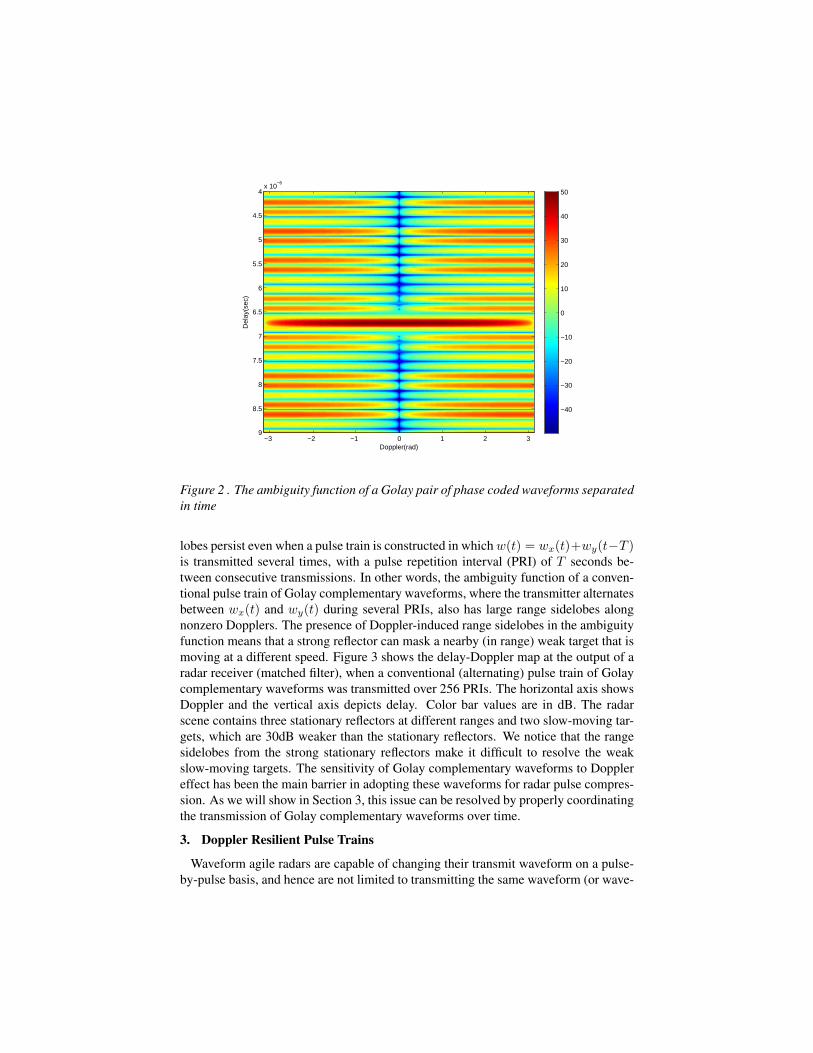
Off the zero-Doppler axis however, the ambiguity function χw(τ, ν) has large side-lobes in delay (range) as Fig. 2 shows. The color bar values are in dB. The range side-

3The shape of the autocorrelation function depends on the autocorrelation function χΩ(τ, 0) for thepulse shape Ω(t). The Golay complementary property eliminates range sidelobes caused by replicas ofχΩ(τ, 0) at nonzero integer delays.

Doppler(rad)

Del

ay(s

ec)

−3 −2 −1 0 1 2 3

4

4.5

5

5.5

6

6.5

7

7.5

8

8.5

9

x 10−6

−40

−30

−20

−10

0

10

20

30

40

50

Figure 2 . The ambiguity function of a Golay pair of phase coded waveforms separatedin time

lobes persist even when a pulse train is constructed in which w(t) = wx(t)+wy(t−T )is transmitted several times, with a pulse repetition interval (PRI) of T seconds be-tween consecutive transmissions. In other words, the ambiguity function of a conven-tional pulse train of Golay complementary waveforms, where the transmitter alternatesbetween wx(t) and wy(t) during several PRIs, also has large range sidelobes alongnonzero Dopplers. The presence of Doppler-induced range sidelobes in the ambiguityfunction means that a strong reflector can mask a nearby (in range) weak target that ismoving at a different speed. Figure 3 shows the delay-Doppler map at the output of aradar receiver (matched filter), when a conventional (alternating) pulse train of Golaycomplementary waveforms was transmitted over 256 PRIs. The horizontal axis showsDoppler and the vertical axis depicts delay. Color bar values are in dB. The radarscene contains three stationary reflectors at different ranges and two slow-moving tar-gets, which are 30dB weaker than the stationary reflectors. We notice that the rangesidelobes from the strong stationary reflectors make it difficult to resolve the weakslow-moving targets. The sensitivity of Golay complementary waveforms to Dopplereffect has been the main barrier in adopting these waveforms for radar pulse compres-sion. As we will show in Section 3, this issue can be resolved by properly coordinatingthe transmission of Golay complementary waveforms over time.

3. Doppler Resilient Pulse Trains

Waveform agile radars are capable of changing their transmit waveform on a pulse-by-pulse basis, and hence are not limited to transmitting the same waveform (or wave-

N=256, Alternating sequence with output in dB

Doppler(rad)

Del

ay(s

ec)

−0.25 −0.2 −0.15 −0.1 −0.05 0 0.05 0.1 0.15 0.2 0.25

1.2

1.3

1.4

1.5

1.6

1.7

1.8

1.9

x 10−5

0

10

20

30

40

50

60

70

80

90

Figure 3 . Delay-Doppler map at the output of a radar receiver (matched filter), whena conventional (alternating) pulse train of Golay complementary waveforms is trans-mitted.

form pair) over time. It is natural to ask whether or not it is possible to exploit this newdegree of freedom to construct a Doppler resilient pulse train (or sequence) of Golaycomplementary waveforms, for which the range sidelobes of the pulse train ambigu-ity function vanish inside a desired Doppler interval. Following the developments in[11]–[13], we show in this section that this is indeed possible and can be achieved bycoordinating the transmission of a Golay pair of phase coded waveforms (wx(t),wy(t))in time according to 1’s and −1’s in a properly designed biphase sequence.

Definition 2: Consider a biphase sequence P = pnN−1n=0 , pn ∈ −1, 1 of length

N , where N is even. Let 1 represent wx(t) and let −1 represent wy(t). The P-pulsetrain wP(t) of (wx(t), wy(t)) is defined as

wP(t) =12

N−1∑n=0

[(1 + pn)wx(t− nT ) + (1− pn)wy(t− nT )] . (10)

The nth entry in wP(t) is wx(t) if pn = 1 and is wy(t) if pn = −1. Consecutiveentries in the pulse train are separated in time by a PRI T .

The ambiguity function of the P-pulse train wP(t), after ignoring the pulse shapeambiguity function and discretizing in delay (at chip intervals), can be written as [13]

χwP (k, θ) =12[Cx(k) + Cy(k)]

N−1∑n=0

ejnθ +12[Cx(k)− Cy(k)]

N−1∑n=0

pnejnθ (11)

where θ = νT is the relative Doppler shift over a PRI. The first term on the right-hand-side of (11) is free of range sidelobes due to the complementary property of Golaysequences x and y. The second term represents the range sidelobes as Cx(k)−Cy(k)is not an impulse. We notice that the magnitude of the range sidelobes is proportionalto the magnitude of the spectrum SP(θ) of the sequence P , which is given by

SP(θ) =N−1∑n=0

pnejnθ. (12)

By shaping the spectrum SP(θ) we can control the range sidelobes. The question ishow to design the sequence P to suppress the range sidelobes along a desired Dopplerinterval. One way to accomplish this is to design P so that its spectrum SP(θ) has ahigh-order null at a Doppler frequency inside the desired interval.

3.1. Resilience to Modest Doppler Shifts

Let us first consider the design of a biphase sequence whose spectrum has a high-order null at zero Doppler frequency. The Taylor expansion of SP(θ) around θ = 0 isgiven by

SP(θ) =∞∑

t=0

1n!

f(t)P (0)(θ)t (13)

where the coefficients f(t)P (0) are given by

f(t)P (0) = jt

N−1∑n=0

ntpn, t = 0, 1, 2, . . . (14)

To generate an M th-order null at θ = 0, we need to zero-force all derivatives f(t)P (0)

up to order M , that is, we need to design the biphase sequence P such that

N−1∑n=0

ntpn = 0, t = 0, 1, 2, . . . ,M. (15)

This is the famous Prouhet (or Prouhet-Tarry-Escott) problem [17],[18], which wenow describe.

Prouhet Problem: [17],[18] Let S = 0, 1, . . . , N − 1 be the set of all integersbetween 0 and N−1. Given an integer M , is it possible to partition S into two disjointsubsets S0 and S1 such that ∑

r∈S0rm =

∑

q∈S1qm (16)

for all 0 ≤ m ≤ M? Prouhet proved that this is possible only when N = 2M+1 andthat the partitions are identified by the Prouhet-Thue-Morse sequence.

Definition 3: [18],[19] The Prouhet-Thue-Morse (PTM) sequence P = (pk)k≥0

over −1, 1 is defined by the following recursions:

1. p0 = 1

2. p2k = pk

3. p2k+1 = −pk

for all k ≥ 0.

Theorem 1 (Prouhet) [17],[18]: Let P = (pk)k≥0 be the PTM sequence. Define

S0 = r ∈ S = 0, 1, 2, . . . , 2M+1 − 1| pr = 0S1 = q ∈ S = 0, 1, 2, . . . , 2M+1 − 1| pq = 1

(17)

Then, (16) holds for all m, 0 ≤ m ≤ M .

We have the following theorem.

Theorem 2: Let P = pn2M−1

n=0 be the length-2M PTM sequence. Then, the spec-trum SP(θ) of P has an (M − 1)th-order null at θ = 0. Consequently, the ambiguityfunction of a PTM pulse train of Golay complementary waveforms (transmitted over2M PRIs) has an (M − 1)th-order null along the zero Doppler axis for all nonzerodelays.

Example 1: The PTM sequence of length 8 is

P = (pk)7k=0 = +1 − 1 − 1 + 1 − 1 + 1 + 1 − 1. (18)

The corresponding pulse train of Golay complementary waveforms is given by

wPTM (t) = wx(t) + wy(t− T ) + wy(t− 2T ) + wx(t− 3T )+wy(t− 4T ) + wx(t− 5T ) + wx(t− 6T ) + wy(t− 7T ). (19)

The ambiguity function of wPTM (t) has a second-order null along the zero-Doppleraxis for all nonzero delays.

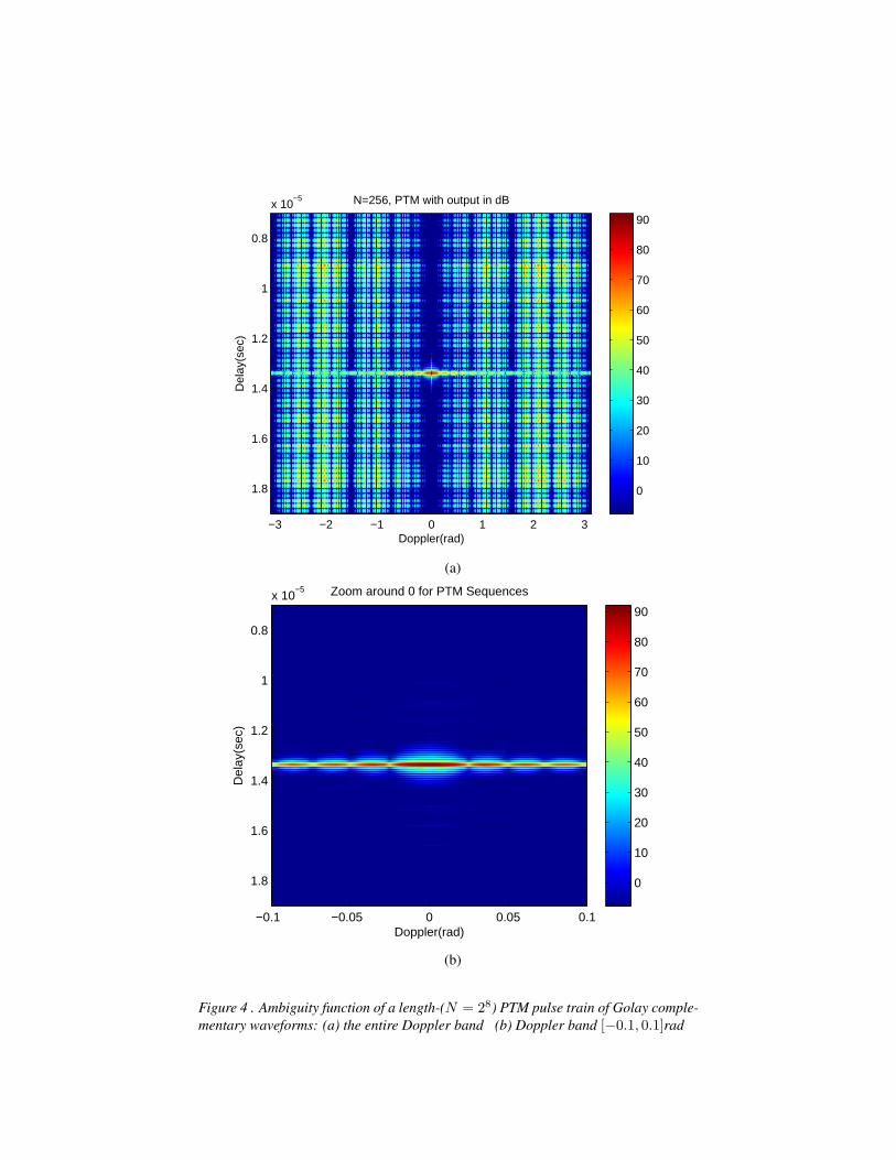
Figure 4(a) shows the ambiguity function of a length-(N = 28) PTM pulse trainof Golay complementary waveforms, which has a seventh-order null along the zero-Doppler axis. The horizonal axis is Doppler shift in rad and the vertical axis is delay insec. The magnitude of the pulse train ambiguity function is color coded and presentedin dB scale. A zoom-in around zero-Doppler is shown in Fig. 4(b). We notice that therange sidelobes inside the Doppler interval [−0.1, 0.1]rad have been cleared out. Theyare at least 80 dB below the peak of the ambiguity function. This means that a PTMpulse train can resolve a weak target that is situated in range near a strong reflector,provided that the difference in speed between the weak and strong scatterers is rela-tively small. Figure 5 shows the ability of the PTM pulse train in bringing out weakslow-moving targets (e.g. pedestrians) in the presence of strong stationary reflectors(e.g. buildings) for the five target scenario discussed earlier in Fig. 3. This exampleclearly demonstrates the value of waveform agility over time for radar imaging. Wenote that the Golay complementary sequences used for phase coding in obtaining Figs.

N=256, PTM with output in dB

Doppler(rad)

Del

ay(s

ec)

−3 −2 −1 0 1 2 3

0.8

1

1.2

1.4

1.6

1.8

x 10−5

0

10

20

30

40

50

60

70

80

90

(a)

Doppler(rad)

Del

ay(s

ec)

Zoom around 0 for PTM Sequences

−0.1 −0.05 0 0.05 0.1

0.8

1

1.2

1.4

1.6

1.8

x 10−5

0

10

20

30

40

50

60

70

80

90

(b)

Figure 4 . Ambiguity function of a length-(N = 28) PTM pulse train of Golay comple-mentary waveforms: (a) the entire Doppler band (b) Doppler band [−0.1, 0.1]rad

N=256, PTM with output in dB

Doppler(rad)

Del

ay(s

ec)

−0.25 −0.2 −0.15 −0.1 −0.05 0 0.05 0.1 0.15 0.2 0.25

1.2

1.3

1.4

1.5

1.6

1.7

1.8

1.9

x 10−5

0

10

20

30

40

50

60

70

80

90

Figure 5 . The PTM pulse train of Golay complementary waveforms can bring outweak targets which would have otherwise been masked by the range sidelobes ofnearby strong reflectors that move at slightly different speeds.

3–5 are of size 64 and the pulse shape is a raised cosine. The chip length is Tc = 100nsec, the carrier frequency is 17 GHz, and the PRI is T = 50 µsec.

3.2. Resilience to Higher Doppler Frequencies

We now consider the design of biphase sequences whose spectra have high-ordernulls at Doppler shifts other than zero. Consider the Taylor expansion of SP(θ) aroundθ = θ0 6= 0:

SP(θ) =∞∑

t=0

1n!

f(t)P (θ0)(θ − θ0)t (20)

where the coefficients f(t)P (θ0) are given by

f(t)P (θ0) =

[dt

dθtSP(θ)

]

θ=θ0

= jtN−1∑n=0

ntpnejnθ0 , t = 0, 1, 2, . . . (21)

We wish to zero-force all the derivatives f(t)P (θ0) up to order M , that is, we wish to

design the sequence P so that

f(t)P (θ0) = 0, for all t = 0, 1, . . . ,M. (22)

Here, we limit our design to rational Doppler shifts θ0 = 2πl/m, where l and m 6= 1are co-prime integers and assume that the length of P is N = mq for some integer q.

If we express 0 ≤ n ≤ N−1 as n = rm+i, where 0 ≤ r ≤ q−1 and 0 ≤ i ≤ m−1,then using binomial expansion for nt = (rm + i)t we can write f

(t)P (θ0) as

f(t)P (θ0) = jt

N−1∑n=0

ntpnejnθ0 (23)

= jt

q−1∑r=0

m−1∑

i=0

(rm + i)tprm+iej(rm+i) 2πl

m (24)

= jt

q−1∑r=0

m−1∑

i=0

t∑u=0

(t

u

)it−u(rm)uprm+ie

j 2πlim (25)

= jtt∑

u=0

(t

u

)mu

m−1∑

i=0

it−uej 2πlim

[q−1∑r=0

ruprm+i

](26)

Define a length-q sequence brq−1r=0 as br = prm+i, 0 ≤ r ≤ q − 1. If brq−1

r=0

satisfiesq−1∑r=0

rubr = 0, for all 0 ≤ u < t (27)

then the coefficient f(t)P (θ0) will be zero. From Theorem 1, it follows that the zero-

forcing condition in (27) will be satisfied if brq−1r=0 is the PTM sequence of length 2t.

We note that f(M)P (θ0) is automatically zero as

∑m−1i=0 ej 2πli

m = 0. Therefore, to zero-force the derivatives f

(t)P (θ0) for all t ≤ M , it is sufficient to select P = pn2

M m−1n=0

such that each prm+iq−1r=0, i = 0, · · · ,m−1 is the length-2M PTM sequence. We call

such a sequence a (2M ,m)-PTM sequence. The (2M ,m)-PTM sequence has length2M × m and is constructed from the length-2M PTM sequence by repeating each 1and −1 in the PTM sequence m times, that is, it is constructed by oversampling thePTM sequence by a factor m.

We have the following theorem.

Theorem 3: Let P = pn2M m−1

n=0 be the (2M ,m)-PTM sequence, that is to sayeach of prm+i2

M−1r=0 , i = 0, · · · ,m − 1 is a PTM sequence of length 2M . Then the

spectrum SP(θ) of P has M th-order nulls at all θ0 = 2πl/m where l and m 6= 1 areco-prime integers.

Corollary 1: Let P be the (2M , m)-PTM sequence. Then the spectrum SP(θ) ofP has an (M − 1)th-order null at θ0 = 0 and (M − h − 1)th-order nulls at all θ0 =2πl/(2hm), where l and m 6= 1 are co-prime, and 1 ≤ h ≤ M − 1.

Proof: The proof for θ0 = 0 is straightforward. For θ0 = 2πl/(2hm), we have

f(t)P (θ0) =

t∑u=0

(t

u

)(2hm)u

2hm−1∑

i=0

it−uej 2πli

2hm

q

2h−1∑r=0

rup2hmr+i

(28)

where q = 2M . The corollary follows from the fact that downsampling a PTM se-quence by a power of 2 produces a PTM sequence of shorter length.

Theorem 3 and Corollary 1 imply that oversampled PTM pulse trains can bring outweak targets which are situated in range near strong reflectors, provided that the rela-tive distance in Doppler shift between the weak and strong scatterers is approximately2πl/(2hm), where l and m 6= 1 are co-prime, and 1 ≤ h ≤ M − 1.

Example 2: The spectrum of the (23, 2)-PTM sequence

P = +1, +1,−1,−1,−1,−1, +1, +1,−1,−1, +1, +1,+1, +1,−1,−1

has a third-order null at θ0 = π rad, a second-order null at θ0 = 0 rad, first-order nullsat θ0 = π/2 rad and θ0 = 3π/2 rad, and zeroth-order nulls at θ0 = (2k + 1)π/4 radfor k = 0, 1, 2, 3. This spectrum is shown in Fig. 6 in solid black line. The spectrumof the (22, 2)-PTM sequence is also shown in this figure in dashed black line. Thisspectrum has a second-order null at θ0 = π rad, a first-order null at θ0 = 0 rad, andzeroth-order nulls at θ0 = π/2 rad and θ0 = 3π/2 rad.

0 0.5 1 1.5 2−100

−80

−60

−40

−20

0

20

Doppler shifts θ/π

|Sp(θ

)|(d

B)

M=3M=2

Figure 6 . The spectra of (23, 2)- and (22, 2)-PTM sequences.

Figure 7(a) shows the ambiguity function of a (28, 3)-PTM sequence of Golay com-plementary waveforms. The color bar values are in dB. This ambiguity function hasan eighth-order null at θ0 = ±2π/3, a seventh-order null at zero Doppler, sixth-ordernulls at θ0 = ±π/3, and so on. A zoom in around θ0 = 2π/3 is provided in Fig. 7(b)to demonstrate that range sidelobes in this Doppler region are significantly suppressed.The range sidelobes in this region are at least 80 dB below the peak of the ambiguityfunction. This example shows the value of properly coordinating the transmission ofcomplementary waveforms over time for achieving a desired ambiguity response.

Doppler(rad)

Del

ay(s

ec)

−3 −2 −1 0 1 2 3

0.8

1

1.2

1.4

1.6

1.8

x 10−5

10

20

30

40

50

60

70

80

90

100

(a)

Doppler(rad)

Del

ay(s

ec)

2 2.02 2.04 2.06 2.08 2.1 2.12 2.14 2.16 2.18 2.2

0.8

1

1.2

1.4

1.6

1.8

x 10−5

5

10

15

20

25

30

35

40

45

50

(b)

Figure 7 . Ambiguity function of the (28, 3)-PTM pulse train of Golay complementarywaveforms: (a) the entire Doppler band (b) Zoom in around θ0 = 2π/3.

4. Instantaneous Radar Polarimetry

Fully polarimetric radar systems are capable of transmitting and receiving on twoorthogonal polarizations simultaneously. The combined signal then has an electricfield vector that is modulated both in direction and amplitude by the waveforms on thetwo polarization channels, and the receiver is used to obtain both polarization compo-nents of the reflected waveform. The use of two orthogonal polarizations increases thedegrees of freedom available for target detection and can result in significant improve-ment in detection performance.

The radar cross section of an extended target such as an aircraft or a ship is highlysensitive to the angle of incidence and angle of view of the sensor (see [20] Sections2.7–8). In general the reflection properties that apply to each polarization componentare also different, and indeed reflection can change the direction of polarization. Thus,polarimetric radars are able to obtain the scattering tensor of a target

Σ =(

σV V σV H

σHV σHH

), (29)

where σV H denotes the target scattering coefficient into the vertical polarization chan-nel due to a horizontally polarized incident field. Target detection is enhanced by con-current rather than serial access to the cross-polarization components of the scatteringtensor, which varies more rapidly in standard radar models used in target detectionand tracking [21] than in models used in remote sensing or synthetic aperture radar[22],[23]. In fact what is measured is the combination of three matrices

H =(

hV V hV H

hHV hHH

)= CRxΣCTx, (30)

where CRx and CTx correspond to the polarization coupling properties of the trans-mit and receive antennas, whereas Σ results from the target. In most radar systemsthe transmit and receive antennas are common, and so the matrices CTx and CRx areconjugate. The cross-coupling terms in the antenna polarization matrices are clearlyfrequency and antenna geometry dependent but for the linearly polarized case thisvalue is typically no better than about -20dB.

In this section, we follow [14],[15] to describe a new approach to radar polarime-try that uses orthogonal polarization modes to provide essentially independent chan-nels for viewing a target, and achieve diversity gain. Unlike conventional radar po-larimetry, where polarized waveforms are transmitted sequentially and processed non-coherently, the approach in [14],[15] allows for instantaneous radar polarimetry (IRP),where polarization modes are combined coherently on a pulse-by-pulse basis. Instan-taneous radar polarimetry enables detection based on full polarimetric properties ofthe target and hence can provide better discrimination against clutter. When comparedto a radar system with a singly-polarized transmitter and a singly-polarized receiverinstantaneous radar polarimetry can achieve the same detection performance (samefalse alarm and detection probabilities) with a substantially smaller transmit energy, oralternatively it can detect at substantially greater ranges for a given transmit energy. In

this section, we present the main idea for waveform transmission in IRP. The reader isreferred to [14],[15] for simulation studies that demonstrate the value of IRP.

4.1. Unitary Waveform Matrices

Let us employ both polarization modes to transmit four phase-coded waveforms w1H ,

w1V , w2

H , w2V . On each polarization mode we transmit two waveforms separated by a

PRI T . We employ Alamouti coding [24] to coordinate the transmission of waveformsover the vertical (V) and horizontal (H) polarization channels; that is, we define

w2H = w1

V (31)

w2V = −w1

H , (32)

where · denotes complex conjugate time-reversal. After discretizing (at chip intervals)and converting time-indexed sequences to z-transform domain, we can write the radarreceive equation in matrix form as

R(z) = z−dHW(z) + Z(z) (33)

where R(z) is the 2 by 2 radar measurement matrix at the receiver, H is the 2 by 2scattering matrix in (30) and Z(z) is a noise matrix. The entries of H are taken to beconstant since they correspond to a fixed range (delay d) and a fixed time. For now,we limit our analysis to zero-Doppler axis and will postpone the treatment of Dopplereffect to Section 4.2. The Alamouti waveform matrix W(z) is given by

W(z) =

(W 1

V (z) −W 1H(z)

W 1H(z) W 1

V (z)

)(34)

where W (z) = zLW (z−1) for a length L sequence w.

If we require the matrix W(z) to be unitary, that is,

W(z)W(z) =

(W 1

V (z) −W 1H(z)

W 1H(z) W 1

V (z)

) (W 1

V (z) W 1H(z)

−W 1H(z) W 1

V (z)

)= 2Lz−L

(1 00 1

)

(35)then it is easy to estimate the scattering matrix H by post-multiplying (33) with W(z).The unitary condition is equivalent to

|W 1V (z)|2 + |W 1

H(z)|2 = 2L. (36)

This is the same condition as the Golay complementary condition and is satisfiedby choosing WV (z) = X(z) and WH(z) = Y (z), where X(z) and Y (z) are z-transforms of the Golay complementary sequences x and y, respectively. This showsthat by properly coordinating the transmission of Golay complementary waveformsacross polarizations and over time we can make the four channels HH, VV, VH, andHV available at the receiver (with delay L) using only linear processing. The fourmatched filters (in z-domain) are given by

Q(z) =(

M1(z)RV (z) M2(z)RV (z)M1(z)RH(z) M2(z)RH(z)

)(37)

where

M1(z) = W 1V (z)z−L − W 1

H(z)

M2(z) = W 1H(z)z−L + W 1

V (z). (38)

and RV (z) denotes the first row of R(z) and represents the z-transform of the entireradar return (over two time slots) received on the vertical polarization channel.

Remark 1: The above description suggests that a radar image will be available onlyon every second pulse, since two PRIs are required to form an image. However, afterthe transmission of the first pulse, images can be made available at every PRI. This isdone by reversing the roles of the waveforms transmitted on the two pulses. Thus, inthe analysis, the matrix W(z) in (33) is replaced by

V(z) =

(−W 1

H(z) W 1V (z)

W 1V (z) W 1

H(z)

)(39)

which is still unitary due to the interplay between Golay property and Alamouti cod-ing. Moreover, the processing involved is essentially invariant from pulse to pulse: thereturn pulse in each of the and channels is correlated against the transmit pulse on thatchannel. This yields an estimate of the scattering matrix on each pulse.

4.2. Doppler Resilient IRP

In the previous section, we restricted our analysis to zero-Doppler axis. Off the zero-Doppler axis, a relative Doppler shift of θ exists between consecutive waveforms oneach polarization channel and the radar measurement equation changes to

R(z) = z−dHW(z)D(θ) + Z(z) (40)

where D(θ) = diag(1, ejθ). Consequently, the unitary property of W(z) can nolonger be used to estimate H, due to the fact that W(z)D(θ)W(z) is not a factor ofidentity. In other words, off the zero-Doppler axis the four elements in W(z)D(θ)W(z)have range sidelobes.

The matrix W(z)D(θ)W(z) can be viewed as a matrix-valued ambiguity function(in z-domain) for IRP. In Section 3, we showed that the range sidelobes of the am-biguity function of a pulse train of Golay waveforms can be suppressed (in a desiredDoppler band) by carefully selecting the order in which the Golay complementarywaveforms are transmitted. This result can be extended to IRP. In fact, it is shownin [11] that the range sidelobes of the IRP matrix-valued ambiguity function can becleared out along modest Doppler shifts by coordinating the transmission of the fol-lowing Alamouti matrices

X1(z) =

(X(z) −Y (z)Y (z) X(z)

)and X−1(z) =

(−Y (z) −X(z)X(z) −Y (z)

)(41)

according to the 1s and −1s in the PTM sequence, where 1 represents X1(z) and−1 represents X−1(z), and X(z) and Y (z) are z-transforms of the Golay pair (x, y).

Range sidelobes along higher Doppler intervals can be cleared out by coordinating thetransmission of X1(z) and X−1(z) according to oversampled PTM pulse trains.

5. Conclusion

In this chapter, we focused on the use and control of degrees of freedom in the radarillumination pattern and presented examples to highlight the value of properly utilizingdegrees of freedom. We showed that by coordinating the transmission of Golay com-plementary waveforms in time (or exploiting waveform agility over time) according tocarefully designed biphase sequences we can construct pulse trains whose ambiguityfunctions have desired properties. We also showed that by combining Alamouti codingand Golay complementary property we can construct unitary polarization-time wave-form matrices that make the full polarization scattering matrix of a target available fordetection on a pulse-by-pulse basis. Looking to the future, we see unitary waveformmatrices as a new illumination paradigm that enables broad waveform adaptabilityacross time, space, frequency and polarization.

6. References

[1] M. I. Skolnik, “An introduction and overview of radar,” in Radar Handbook,M. I. Skolnik, Ed. New York: McGraw-Hill, 2008.

[2] M. C. Wicks, M. Rangaswamy, R. Adve, and T. B. Hale, “Space-time adaptiveprocessing,” IEEE Signal Processing Magazine, no. 1, pp. 51–65, Jan. 2006.

[3] M. J. E. Golay, “Multislit spectrometry,” J. Opt. Soc. Am., vol. 39, p. 437, 1949.

[4] ——, “Static multislit spectrometry and its application to the panoramic displayof infrared spectra,” J. Opt. Soc. Am., vol. 41, p. 468, 1951.

[5] ——, “Complementary series,” IRE Trans. Inform. Theory, vol. 7, no. 2, pp.82–87, April 1961.

[6] G. R. Welti, “Quaternary codes for pulsed radar,” IRE Trans. Inform. Theory, vol.IT-6, no. 3, pp. 400–408, June 1960.

[7] M. R. Ducoff and B. W. Tietjen, “Pulse compression radar,” in Radar Handbook,M. I. Skolnik, Ed. New York: McGraw-Hill, 2008.

[8] C. C. Tseng and C. L. Liu, “Complementary sets of sequences,” IEEE Trans.Inform. Theory, vol. IT-18, no. 5, pp. 644–652, Sep. 1972.

[9] R. Sivaswami, “Multiphase complementary codes,” IEEE Trans. Inform. Theory,vol. IT-24, no. 3, pp. 546–552, Sept. 1978.

[10] R. L. Frank, “Polyphase complementary codes,” IEEE Trans. Inform. Theory,vol. IT-26, no. 6, pp. 641–647, Nov. 1980.

[11] A. Pezeshki, A. R. Calderbank, W. Moran, and S. D. Howard, “Doppler resilientGolay complementary waveforms,” IEEE Trans. Inform. Theory, vol. 54, no. 9,pp. 4254–4266, Sep. 2008.

[12] ——, “Doppler resilient Golay complementary pairs for radar,” in Proc. Stat.Signal Proc. Workshop, Madison, WI, Aug. 2007, pp. 483–487.

[13] S. Suvorova, S. D. Howard, W. Moran, R. Calderbank, and A. Pezeshki,“Doppler resilience, Reed-Muller codes, and complementary waveforms,” inConf. Rec. Forty-first Asilomar Conf. Signals, Syst., Comput., Nov. 2007, pp.1839–1843.

[14] S. D. Howard, A. R. Calderbank, and W. Moran, “A simple polarization diversitytechnique for radar detection,” in Proc. Second Int. Conf. Waveform Diversityand Design, Lihue, HI, Jan. 2006.

[15] ——, “A simple signal processing architecture for instantaneous radar polarime-try,” IEEE Trans. Inform. Theory, vol. 53, pp. 1282–1289, Apr. 2007.

[16] N. Levanon and E. Mozeson, Radar Signals. New York: Wiley, 2004.

[17] E. Prouhet, “Memoire sur quelques relations entre les puissances des nombres,”C. R. Acad. Sci. Paris Ser., vol. I 33, p. 225, 1851.

[18] J. P. Allouche and J. Shallit, “The ubiquitous Prouhet-Thue-Morse sequence,” inSequences and their applications, Proc. SETA’98, T. H. C. Ding and H. Nieder-reiter, Eds. Springer Verlag, 1999, pp. 1–16.

[19] M. Morse, “Recurrent geodesics on a surface of negative curvature,” Trans. Amer.Math Soc., vol. 22, pp. 84–100, 1921.

[20] M. I. Skolnik, Introduction to Radar Systems, 3rd ed. McGraw-Hill, 2001.

[21] H. L. V. Trees, Detection, Estimation and Modulation Theory, Part III. NewYork: Wiley, 1971.

[22] R. K. Moore, “Ground echo,” in in Radar Handbook, M. I. Skolnik, Ed. NewYork: McGraw-Hill, 2008.

[23] R. Sullivan, “Synthetic aperture radar,” in in Radar Handbook, M. I. Skolnik, Ed.New York: McGraw-Hill, 2008.

[24] S. Alamouti, “A simple transmit diversity technique for wireless communica-tions,” IEEE J. Select. Areas Commun., vol. 16, no. 8, pp. 1451–1458, Oct. 1998.