Communication Systems, 5e

Chapter 9: Random Signals and Noise

A. Bruce CarlsonPaul B. Crilly

© 2010 The McGraw-Hill Companies

Chapter 9: Random Signals and Noise

• Random processes• Random signals• Noise• Baseband signal transmission with noise• Baseband pulse transmission with noise

© 2010 The McGraw-Hill Companies

3

Copyright © The McGraw-Hill Companies, Inc. Permission required for reproduction or display.

Waveforms in an ensemble v(t,s)Figure 9.1-1

Ensemble

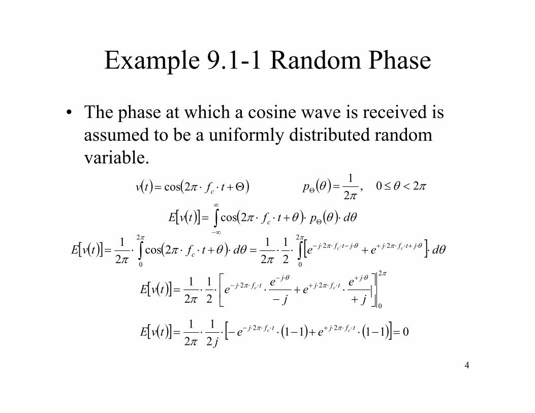
Example 9.1-1 Random Phase

• The phase at which a cosine wave is received is assumed to be a uniformly distributed random variable.

4

tftv c2cos

20,21

p

dptftvE c2cos

2

0

222

0 21

212cos

21 deedtftvE jtfjjtfj

ccc

2

0

22

21

21

jee

jeetvE

jtfj

jtfj cc

0111121

21 22 tfjtfj cc ee

jtvE

5

Random Digital Signal

• A random digital waveform based on a rectangular pulse train with bit/symbol period D– The time delay is a continuous RV uniformly distributed between 0

and the pulse width D– The amplitude of the kth pulse is a discrete RV with zero mean and

a known variance. – The amplitudes during different intervals are independent (i.i.d)

k

dk D

DkDTtrectatv 2

DT0,D1Tp dd

kjfor,0aaE

aE,0aE

kj

22nn

Random Digital Signal (2)

6

k

dk D

DkDTtrectatv 2

7

Random Digital Signal

• Autocorrelation

• Power Spectral Density

DD,D

1tvtvER 2vv

DfcsinDtvtvEwS 22vv

8

Copyright © The McGraw-Hill Companies, Inc. Permission required for reproduction or display.

(a) Sample function; (b) Autocorrelation; (c) Power spectrum: Figure 9.2-3

Random Telegraph: Example 9.2-1

• Poisson distribution– Average number of

transitions per unit time– DC component

9

Random Telegraph: Example 9.2-1

• Poisson distribution

t2exp14

AR2

vv

4A

4A

4A2

2exp14

A02exp14

A

tvEtvE

2222

vv

222

vv

222vv

f4

A

f14

AfS2

2

2

vv

10

Modulation

• Typical receivers have a random phase offset in the carrier. Uniform distribution.

tf2costvtz c

20,21p

cvvzz f2cosR21R

cvvcvvzz ffSffS41fS

11

Linear Filtering

• Filtering of random variables xxyx RhR

xxyy RhhR

fSfHfHfS xxyy

fSfHfS xxyy 2

12

Thermal Noise Power

• Noise produced by the random motion of charge particles in conducting media

• Modeled as additive white Gaussian noise (AWGN)

– Where κ is Boltzmann’s constant– T is absolute temperature in degrees Kelvin– B is the bandwidth in Hertz

BTN

HzK/dBW6.228

refIEEEK290T0

21e00.429023e38.1TN 00

Hz/dBm174Hz/dBW204N0

Thermal Resistance Noise

© 2010 The McGraw-Hill Companies

(a) Thevenin Voltage Model

(b) Norton Current Model

Resistor Models with Noise PSD

14

Noise Approximation

• Uniform Noise Spectral Density– Resistor description (Thevenin Model)

• Available Power from the “noise source”– Source output power into a matched load

TR2fGvv

ssout vR2

Rv

R4

vR1

2v

RvP

2s

2s

2sout

sout

2

N2T

R4TR2

R4fGfG 0vv

ss

2

NR 0ss

15

System Noise

• Since the noise power spectrum is uniform, a systems noise power is the product of the noise power and the integral of the filter power.

20NN

2NN fH

2NfSfHfS

00

0

20

20NN dffHNdffH

2N0R

Noise Equivalent Bandwidth

• If we want the total noise power after the filter, we can integrate the PSD for all frequencies or use the Filtered noise autocorrelation function at zero.– Both of these approaches may be difficult– Could we generate a more simple “noise equivalent

bandwidth for filters” that is rectangular?

16

17

EQNEQNPowerDCelrect BHBGaindffHdffH

2_

0

2

mod_0

2 0

EQNPowerDCelrect B

frectGainfH2_mod_

20

2

EQN0H

dffHB

2Power_DC 0HGain

Noise Equivalent Bandwidth

0

2020NN dffH2

2NdffH

2N0R

• When filtering, it is convenient to think of band-limited noise, where the filter is a rect function with bandwidth BEQN

18

Noise Equivalent Bandwidth

• Low pass filter 0Hgain_coherent

• For a unity gain filter – assumed when computing receiver input noise power

EQN0EQN0

NNN BNB22

N0RP

2Power_DC 0HGain

20

2

EQN0H

dffHB

0

2EQN dffHB

EQN02

EQN20

NNN BN0HB0H22

N0RP

Model of Received Signal with Noise

© 2010 The McGraw-Hill Companies

20

Copyright © The McGraw-Hill Companies, Inc. Permission required for reproduction or display.

Analog baseband transmission system with noise: Figure 9.4-2

Signal Plus Noise

• Additive Gaussian White Noise

ttf2costAtx c

ttfLtAtx cR 2cos tnttf

LtAts c 2cos

thtnttfLtAteD c

2cosPr

21

Signal-to-Noise Ratio

• Comparing the desired signal power to the undesired noise power.

• To compare signal and noise power, we must assume a filtering operations

tntxty c

TransmittingAntenna

ReceivingAntenna

RF Communication Channel

Noise

Linear Filtering

NonlinearDistortion

Atten-uation

tn

txc

tntxty c

22

Signal-to-Noise Ratio

• Equivalent receiver input signal and noise (ER)

• Equivalent destination signal and noise (D) or pre-demodulation (PreD)

thtntxty RD

tntxty ERERR

tntxty eDeDeD PrPrPr

23

Signal-to-Noise Ratio

• Equivalent receiver input SNR (ER)

EQN

R

EQN

ER

ER

ERR BN

SBNtxE

tnEtxESNR

00

2

2

2

• Equivalent destination SNR EQN

D

D

D

eD

eDR BN

SNS

tnEtxESNR

02

Pr

2Pr

can be used to represent receiver noise figure contributions

24

Increase in SNR with filtering

• If a filter matched to the input signal is applied, the noise power would be reduced to the smallest equivalent noise bandwidth that is allowed.– Filter to minimize noise power– Importance of the IF filter in a super-het receiver!

• Front-end filtering goals – a dilemna– Minimize signal power loss (wider bandwidth)– Minimize filter equivalent noise bandwidth

(narrower bandwidths)– A trade-off must be made!

25

Typical Transmission Requirements

Signal Type Freq. Range SNR (dB)Intelligible Voice 500 Hz to 2 kHz 5-10Telephone Quality 200 Hz to 3.2 kHz 25-35AM Broadcast Audio 100 Hz to 5 kHz 40-50High-fidelity Audio 20 Hz to 20 kHz 55-65Video 60 Hz to 4.2 MHz 45-55Spectrum Analyzer 100 kHz-1.8 GHz 65-75

Pulse Measurement in Noise

© 2010 The McGraw-Hill Companies

© 2010 The McGraw-Hill Companies

Pulse Measurement in Noise 2

0

Let received pulse be a rectangle with amplitude, duration, energy, and zero mean noise with PSD ( ) / 2

LPF 1/ 2

At the filter output ( ) ( )where

p

N

a a A

A

A E AG f N

B B

y t A n t Aamplitude

2 20

22 0 0Lower bound on error variance

2 2

Achieving lower bound

A N

Ap

error

n N B

N N AE

matched filter

AAy

Note: y is a random variable with a variance and pdf

Time-position Error Caused By Noise

© 2010 The McGraw-Hill Companies

• Time error rv relation

• Time error variance

222

br

tt tnAtEE

At

tnr

b

t

Time-position Error Caused By Noise (2)

• Time Position Error Variance

• Matching the transmit bandwidth

• Therefore

© 2010 The McGraw-Hill Companies

Nr

br

tt BNAttn

AtEE

0

2222

pEA 2

Tr Bt

21

NTTp

Nt BBfor

BEBN

,4 2

02

NTTTp

t BBforBA

NBE

N

,44 2

002

tmeasureedge tt

30

Matched Filter

• See Chapter 9 of ECE 3800 Text– Notes are on the web site