1

CHAPTER 9: MASS-BALANCE MODELING

9.1 OVERVIEW

Chapter 3 describes 1998 load calculations for each tributary and water-quality

component. This chapter integrates these results into a mass-balance framework for the

Lake as a whole (Figure 9-1). Mass balances provide important information on sources

controlling water quality, foundations for empirical and mechanistic modeling, and bases

for tracking watershed and lake responses to implementation of control measures.

Interactive software has been developed to perform the following functions for a user-

specified water quality component and season (calendar year, water year, growing

season):

• Summarize water and mass balances for specified year or year range;

• Estimate the uncertainty (standard error) of each mass-balance term;

• Refine the monitoring program design to reduce uncertainty in load estimates;

• Track trends in each mass-balance term (individual sources, total inputs & outputs);

• Calibrate empirical mass-balance models to forecast responses of lake outflow

concentrations and loads to variations in inflow volumes and loads.

The software is currently set up to analyze 1986-1998 data for the following monitored

water quality components:

• Phosphorus species (total, total inorganic, ortho)

• Nitrogen species (total, kjeldahl, nitrate, nitrite, ammonia)

• Carbon species (total organic, total inorganic)

• Biochemical Oxygen Demand

• Total Suspended Solids

• Inorganic species (chloride, sodium, calcium, alkalinity)

• Fecal Coliforms

2

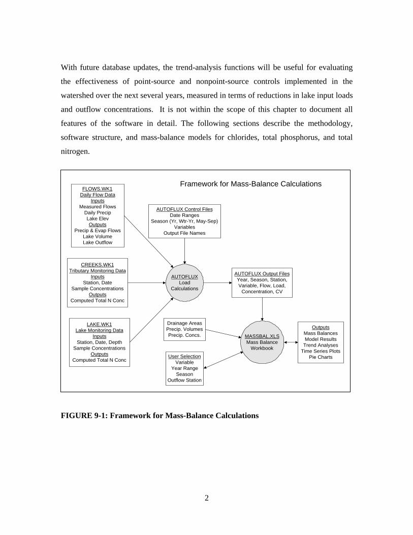
With future database updates, the trend-analysis functions will be useful for evaluating

the effectiveness of point-source and nonpoint-source controls implemented in the

watershed over the next several years, measured in terms of reductions in lake input loads

and outflow concentrations. It is not within the scope of this chapter to document all

features of the software in detail. The following sections describe the methodology,

software structure, and mass-balance models for chlorides, total phosphorus, and total

nitrogen.

FIGURE 9-1: Framework for Mass-Balance Calculations

FLOWS.WK1Daily Flow Data

InputsMeasured Flows

Daily PrecipLake ElevOutputs

Precip & Evap FlowsLake VolumeLake Outflow

CREEKS.WK1Tributary Monitoring Data

InputsStation, Date

Sample ConcentrationsOutputs

Computed Total N Conc

AUTOFLUXLoad

Calculations

AUTOFLUX Output FilesYear, Season, Station,Variable, Flow, Load,

Concentration, CV

AUTOFLUX Control FilesDate Ranges

Season (Yr, Wtr-Yr, May-Sep)Variables

Output File Names

OutputsMass BalancesModel Results

Trend AnalysesTime Series Plots

Pie Charts

LAKE.WK1Lake Monitoring Data

InputsStation, Date, Depth

Sample ConcentrationsOutputs

Computed Total N Conc

Drainage AreasPrecip. VolumesPrecip. Concs.

Framework for Mass-Balance Calculations

User SelectionVariable

Year RangeSeason

Outflow Station

MASSBAL.XLSMass Balance

Workbook

3

9.2 METHODOLOGY

Basic data for the calculations are stored in three worksheet files:

• FLOWS.WK1 - daily measured flows (creeks, point sources, precipitation), measured

elevations, & calculated flows (ungauged inputs, outflows).

• CREEKS.WK1 - tributary & point-source concentration data (1985-1998)

• LAKE.WK1 - lake concentration data (1968-1998)

The data worksheets are in formats that are compatible with AUTOFLUX (used in

Chapter 3 for load calculations), FLUX (interactive software for load calculations,

Walker (1996)), and TRENDS (used in Chapters 3 & 4 for trend analyses).

Daily water balances are computed in FLOWS.WK1. Table 9-1 describes the algorithm

TABLE 9-1: Water Balance Algorithm

Outflow = Inflows + Precipitation - Evaporation - Increase in Storage Inflows:

Tributaries Gauged: Onondaga, Harbor, Ley, Ninemile

Ungauged ~ 0.051 x Gauged Industrial

Allied / East Flume, Crucible Municipal

Metro Effluent & Bypass

Precipitation: Daily Precipitation x Lake Area

Daily Precip. from Hancock Airport (~38 in/yr)

Evapotranspiration: Daily Evaporation x Lake Area

Regional Average Monthly Evaporation Data (~27 inches/yr) (VanderLeden et al., 1990)

Increase in Storage:

Daily Increase in Elevation x Lake Area

Outflow Time Series Smoothed (7 Day Rolling Average)

4

for computing daily lake outflow volumes.

Based upon drainage areas reported by the USGS (Table 9-2), about 14.3 mi2 of the

watershed is ungauged (above Lake and below USGS gauges). Gauged watershed

inflows are multiplied by the ungauged/gauged drainage area ratio (.051) to estimate

ungauged inflows and loads. Development of a GIS coverage for the watershed (e.g.,

Figure 1-5) is recommended to refine drainage area estimates above each gauge and

above the lake as a whole.

TABLE 9-2: Drainage Areas

USGS Station

Number

Drainage

Area (mi2)

Onondaga/Spencer 04240010 110.0

Ley/Park 04240120 29.9

Harbor/Hiawatha 04240105 11.3

Ninemile/Lakeland 04240300 115.0

Ungauged (calculated) 14.3

Lake 4.5

Total 04240495 285.0

Onondaga/Dorwin 04239000 88.5

Harbor /Velasko 04240100 10.0

AUTOFLUX (Walker, 1995) computes loads for each monitored inflow, season, year,

and water-quality component. Three alternative estimates of lake outflow loads are

computed by pairing daily outflow volumes with monitored concentrations at each of

three locations (Outlet @ 2 feet, Outlet @ 12 feet, Lake South Epilimnion (<9 meters).

In years following elimination of saline discharges from the Allied Chemical facility,

yearly chloride balances (see below) are tightest using the Outlet @ 2 feet. AUTOFLUX

generates ASCII output files that are subsequently pasted into the Excel-97 workbook

used for mass-balance calculations and analysis (MASSBAL.XLS, Figure 9-1).

5

Data inputs to the load-calculation workbook include:

• AUTOFLUX output files (see above)

• Drainage area estimates (Table 9-2)

• Precipitation volumes for each year and season (from Hancock Airport)

• Rainfall concentrations for estimating atmospheric inputs (Table 9-3)

The workbook is currently stoked with results for 1986-1998, three seasons (calendar

year, water year, May-September), and variables listed in Section 9.1. Pending results of

further data screening for 1990-1997, concentration outliers detected by AUTOFLUX at

the 0.01 significance level have been excluded from load calculations. Future data can be

pasted into the workbook to update the calculations.

To facilitate long-term trend analyses, missing historical data have been estimated as

follows:

• Total P, All Terms, 1986-1989. Estimated from Total Inorganic Phosphorus loads

using TP/TIP ratios for each term derived from years when both TP and TIP were

measured (between 1990 & 1997, depending on term).

• All Variables, Crucible, 1992. Estimated using concentrations measured in 1991.

• Metro Bypass, All Variables, 1986-1992. Estimated using measured flows in each

year and flow-weighted-mean concentrations measured in 1994-1998. A search for

1986-1992 bypass concentration data is recommended.

Although tributary concentration data are available for 1985, the flow record is

incomplete. Compilation of daily flows for Metro effluent and bypass would enable

mass-balance computations for 1985. Load estimates for 1985 currently in the

workbook use 1986 daily flows for the effluent and bypass.

Nominal estimates of rainfall concentration for each water quality component are listed in

Table 9-3. These values can be refined with additional literature review. The

6

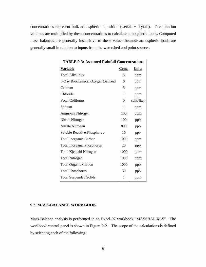
concentrations represent bulk atmospheric deposition (wetfall + dryfall). Precipitation

volumes are multiplied by these concentrations to calculate atmospheric loads. Computed

mass balances are generally insensitive to these values because atmospheric loads are

generally small in relation to inputs from the watershed and point sources.

TABLE 9-3: Assumed Rainfall Concentrations

Variable Conc. Units

Total Alkalinity 5 ppm

5-Day Biochemical Oxygen Demand 0 ppm

Calcium 5 ppm

Chloride 1 ppm

Fecal Coliforms 0 cells/liter

Sodium 1 ppm

Ammonia Nitrogen 100 ppm

Nitrite Nitrogen 100 ppb

Nitrate Nitrogen 800 ppb

Soluble Reactive Phosphorus 15 ppb

Total Inorganic Carbon 1000 ppm

Total Inorganic Phosphorus 20 ppb

Total Kjeldahl Nitrogen 1000 ppm

Total Nitrogen 1900 ppm

Total Organic Carbon 1000 ppb

Total Phosphorus 30 ppb

Total Suspended Solids 1 ppm

9.3 MASS-BALANCE WORKBOOK

Mass-Balance analysis is performed in an Excel-97 workbook "MASSBAL.XLS". The

workbook control panel is shown in Figure 9-2. The scope of the calculations is defined

by selecting each of the following:

7

• Water quality variable

• Season (May-September, Calendar Year, or Water Year)

• Lake Outlet Station (Outlet @ 2 feet, Outlet @ 12 feet, or Lake South Epilimnion)

• Model Formulation (Constant Settling Rate, or Constant Retention Coefficient, each

calibrated to a selected date range or specified by the user)

• Calibration Year Range (used in model calibration & detailed mass-balance table)

• Total Year Range (used in model testing & trend analyses)

FIGURE 9-2: MASSBAL.XLS Control Panel

With the scope selected, a variety of graphs and tables can be viewed. To view a graph,

select the desired graph name from the list and then click the 'View Graph' button. Hit

'Cntrl-m' to return to the control panel after viewing any graph or table. A brief

description of each graph format (Table 9-4) and table format (Table 9-5) can be

accessed by clicking the 'Glossary' button on the control panel.

8

TABLE 9-4 : List of Output Graphs

Graph Description

Inflow_Volumes Bar Chart of Inflow Volumes in Each Source Category

Inflow_Loads Bar Chart of Inflow Loads in Each Source Category

Load_Variance Bar Chart of Load Variances in Each Source Category

Load_Trends Trends in Total Inflow & Total Outflow Loads

Load_Source_Trends Trends in Municipal & Non-Point Loads

Conc_Trends Trends in Total Inflow & Total Outflow Concentrations

FlowAdjConc_Trends Trends in Total Inflow & Total Outflow Flow-Adjusted Concs

FlowAdjLoad_Trends Trends in Total Inflow & Total Outflow Flow-Adjusted Loads

Load_InOut Bar Chart of Total Inflow & Total Outflow Loads

Load_InOutRet Bar Chart of Total Inflow Loads , Outflow Loads, and Retention

LoadOut_LoadIn Scatter Plot of Outflow Loads vs. Inflow Loads

Conc_InOut Bar Chart of Total Inflow & Outflow Concs

Conc_Outlets Bar Chart of Total Inflow & Outflow Concs for Alt. Outlets

ConcOut_ConcIn Scatter Plot of Outflow Concs vs. Inflow Concs

Non_Point Unit Area Flows, Loads, & Concs. for Each Watershed

Pie_Flows Pie Chart of Inflow Volumes by Source

Pie2_Flows Pie Chart of Inflow Volumes by Source Category

Pie_Loads Pie Chart of Inflow Loads by Source

Pie2_Loads Pie Chart of Inflow Loads by Source Category

Pie_Variance Pie Chart of Inflow Load Variance by Source Category

Model_Conc Observed & Predicted Outflow Concentrations

Model_Load Observed & Predicted Outflow Loads

Model_Param Water Load, Setting Rates, Retention Coef.

Model_Diagnostics Model Residuals Plots

Model_Epil Summer Epilimnetic Total Phosphorus or Total Nitrogen Model

9

TABLE 9-5 : List of Output Tables

Table Description

Sample_Counts Number of Samples vs. Station & Year

Detailed Mass-Balance Complete Water & Mass Balance

Trend_Summary Summary of Trends in Major Mass-Balance Terms

Trends_All Summary of Trends in Flows, Loads, & Concs for Each Term

Trends_Flows Trend Analysis Details - Flows

Trends_Loads Trend Analysis Details - Loads

Trends_Concs Trend Analysis Details - Concentrations

Trends_FlowAdjLoads Trend Analysis Details - Flow-Adjusted Loads

Trends_FlowAdjConcs Trend Analysis Details - Flow-Adjusted Concentrations

Trend_CrossTab_Loads Summary of Load Trends vs. Variable & Mass-Balance Term

Trend_CrossTab_Concs Summary of Conc. Trends vs. Variable & Mass-Balance Term

Model_Calcs Mass-Balance Model Calculations

Model_Applic Apply Mass-Balance Model to Hypothetical Load Scenario

Model_CrossTab Summary of Model Results vs. Variable & Model Formulation

Inputs_AUTOFLUX AUTOFLUX Output Data

Inputs_DrainageAreas Input Drainage Areas

Inputs_Precip Input Precipitation Data

Inputs_VariableIndex Input Variable Names & Rainfall P Concs.

9.3 TREND ANALYSIS METHODS

The "Select Term" menu on the far right of the control panel (Figure 9-2) lists yearly time

series and performs a trend analysis any term of the mass balance. Trend analyses for

total inputs and total outputs can also be viewed from graph and table menu. Trends are

evaluated via linear regression against year. Tests are performed for flow, load,

concentration, flow-adjusted load, and flow-adjusted concentration.

Flow-adjusted values remove a portion of the hydrologic variability from the time series.

In situations where load or concentration are significantly correlated with flow, adjusted

values may provide an improved basis for detecting trends, expressed in terms of higher

10

power and less risk that hydrologic variations will be mistakenly interpreted as long-term

trends (Hirsch et al., 1982). This is particularly true for loads, since correlations between

load and flow are generally stronger than correlations between concentration and flow.

Flow-adjusted concentrations are computed as follows:

Ca = C + bc ( Qm - Q )

where,

Ca = flow-adjusted concentration for current year (ppb)

C = measured flow-weighted-mean concentration for current year (ppb)

bc = slope of concentration vs. flow regression

Q = average flow for current year (106 m3/yr)

Qm = average flow for entire time series (106 m3/yr)

Measured yearly concentrations are adjusted to average flow conditions based upon the

slope of the concentration vs. flow regression. Future investigation of alternative forms

for the concentration vs. flow regression (e.g., log-scale or polynomial) is suggested.

Analogous equations are used to compute flow-adjusted loads.

If there is a long-term trend in flow over the tested year interval, flow-adjusted results

should be interpreted cautiously. In this situation, the correlation between flow and year

makes it difficult to distinguish their effects on concentration or load. The above

procedures for filtering out apparent flow-related variations will also tend to filter out any

long-term trends and cause a Type II error (failure to detect a real trend). Lake inflow

volumes and loads between 1986 and 1998 are shown in Figures 9-3 and 9-4,

respectively. Because of the high flow in 1990 and low-to-average flows in 1995, 1997,

and 1998, distinguishing flow effects from long-term trend would be relatively difficult

for trend analyses between 1990 and 1998. In such situations, the unadjusted

concentration time series is probably more reliable as a trend indicator.

11

FIGURE 9-3: Long-Term Variations in Lake Inflow Volume

FIGURE 9-4: Long-Term Variations in Total Phosphorus Load

12

The 'Trend CrossTab' table summarizes significant trends in each variable and mass-

balance term. These tables must be manually updated if the year interval for trend

analysis or the outlet definition is changed. Updating is accomplished by clicking the

'Update CrossTabs' button (Figure 9-2). Tables 9-6 and 9-7 show trend crosstabs for

concentrations and loads between 1986 and 1998. Values in the table represent trend

magnitudes (% per year) that are significant at p < .10 (two-tailed test).

9.4 MASS-BALANCE MODELING

The software facilitates calibration and testing of empirical mass-balance models for

predicting lake outflow concentrations as a function of inflow volumes and loads. The

following alternative model formulations are considered:

Constant Settling Velocity (Chapra & Tarapchak, 1976):

Co = Ci Qs / ( Qs + U )

Constant Retention Coefficient (Dillion & Rigler, 1975):

Co = Ci ( 1 - R )

where,

Co = Lake outflow concentration (ppb)

Ci = Average inflow concentration = Wi / Qo

Wi = Inflow load (kg/yr)

Qo = Lake outflow (106 m3/yr)

Qs = Water load (m/yr) = Qo / A

R = Retention coefficient

U = Net Settling Velocity (m/yr)

The empirical parameters (U or R) can be calibrated to average mass balances for the

specified calibration years or estimated independently by user.

13

Model performance for predicting outflow concentration or load over the entire period is

measured by the explained variance (r2) and residual standard error, expressed as a

percentage of the predicted value (CV%). In applications to phosphorus & nitrogen

discussed below, models are calibrated to the most recent five-year period (1994-1998)

and tested against 1986-1998 yearly time series. Predictions for 1986-1993 provide

independent verification of the models calibrated to average 1994-1998 mass-balances.

Model output is represented in tables and figures labeled "model_" (e.g., 'model_concs'

shows observed & predicted outflow concentrations, along with calibrated parameters

and performance measures).

For both phosphorus and nitrogen, there is some possibility that the lake response to

nonpoint loads is different from its response to point-source loads. This would be

reflected in terms of different retention coefficients or settling velocities for each source

category. Unfortunately, testing this hypothesis is not straight-forward because year-

year-variations in the ratio of point-source to nonpoint-source loads are strongly

correlated with year-to-year variations in flow. Point sources tend to represent a lower

percentage of the total load during wet years. This makes it difficult to distinguish effects

of hydrologic variations from differential responses to point vs. nonpoint loads.

Residuals from the models discussed below are generally uncorrelated with

point/nonpoint load ratios. Further investigations of this aspect are recommended,

however.

14

9.5 CHLORIDE BALANCE MODEL

Assuming that chlorides are conservative, input and output loads should be

approximately equal. Comparing input and output loads provides a basis for testing the

testing the overall water balance and testing the scheme for estimating ungauged flows

and loads. The 1994-1998 chloride balance is listed in Table 9-8. In this period, total

input and output loads differ by 1% using the 2-foot samples to compute outflow loads,

as compared with 20% using the 20-foot outlet samples and 18% using the Lake South

epilimnetic concentrations. Lack of consistent year-round sampling limits the usefulness

of the Lake South data for computing outflow loads. Observed and predicted yearly

outflow chloride loads are shown in Figure 9-5, based upon the mass-balance model with

an assumed settling velocity of 0.0 m/yr. The model explains 78% of the observed

outflow load time series with a residual standard error of 16%. Based upon these results,

2-foot outlet samples are used below in developing phosphorus and nitrogen balances.

15

FIGURE 9-5: Observed & Predicted Outflow Chloride Loads

16

9.6 PHOSPHORUS BALANCE MODEL

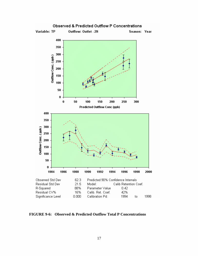
Table 9-9 lists the total phosphorus balance for the 1994-1998 period. The lake retained

41.6% of the input phosphorus load, corresponding to an average settling of 25.9 m/yr.

Figure 9-6 shows observed and predicted yearly-average outflow concentrations for

1986-1998 using the retention coefficient calibrated to 1994-1998 data (41.6%). The

constant-retention model (r2 = 86%, residual CV = 16%) performs slightly better than the

constant settling-rate model (r2 = 79%, residual CV = 21%). As discussed above (see

9.2), total phosphorus concentrations and loads for 1986-1989 have been estimated from

total inorganic phosphorus values. The resulting equation for predicting yearly-average

outflow phosphorus concentration is:

Po = PI ( 1 - R ) = 0.584 PI

90% Confidence Interval = [0.42 to 0.75 ] PI

Summer epilimnetic phosphorus concentrations are of primary concern for evaluating

lake trophic state. Observed values have been computed using 0 to 6 meter samples

collected from June through September at the Lake South station. Sample results have

been averaged by date before computing a mean and standard error for each year. Table

9-10 lists summer-mean epilimnetic concentrations for each year between 1986-1998,

along with annual phosphorus balance terms.

The yearly phosphorus-balance model can be extended to predicted summer epilimnetic

concentrations using an equation of the following form:

Ps = k Po = k ( 1 - R ) Pi

where,

Ps = summer epilimnetic total phosphorus concentration (ppb)

k = proportionality constant = 0.657 (calibrated)

17

FIGURE 9-6: Observed & Predicted Outflow Total P Concentrations

18

TABLE 9-10: Summary of Lake Phosphorus Balances, 1986-1998

Note: Total P values for 1986-1989 estimated from Total Inorganic P values.

InflowOutflow Conc

Year 10^6 m3 kg RSE% kg RSE% ppb ppb RSE% ppb RSE%1986 520.1 219291 5% 160823 7% 422 221 11% 188 8%1987 372.0 172524 5% 139721 6% 464 237 13% 157 6%1988 344.2 145301 5% 113725 5% 422 276 8% 170 8%1989 472.8 138328 8% 83672 11% 293 146 20% 108 21%1990 654.7 136496 7% 68521 10% 208 122 12% 88 14%1991 427.0 93004 8% 59151 11% 218 91 11% 61 9%1992 516.6 88792 7% 60056 9% 172 109 10% 62 18%1993 535.4 148006 5% 106586 6% 276 165 7% 132 12%1994 475.5 98233 10% 68941 11% 207 104 13% 87 11%1995 307.0 60025 5% 44741 3% 196 136 8% 72 13%1996 530.1 98179 5% 55265 3% 185 116 8% 68 10%1997 362.6 49448 3% 34160 2% 136 94 10% 56 10%1998 449.9 71681 7% 43021 2% 159 75 9% 55 8%

94-98 425.0 75513 6% 49226 4% 178 104 10% 67.8 10%

RSE = relative standard error = standard error / mean

Summary of Lake Phosphorus BalancesCalendar Years 1986-1998

@ 2 ftOutflow Conc

Lake South Epil.June-Sept, 0-6 m

Inflow Load ConcentrationMetro+Bypass Load

19

With k and R values calibrated to 1994-1998 data, the resulting equation is:

Ps = 0.657 ( 1 - 0.416 ) = 0.384 PI,

90% Confidence Interval = [0.28 to 0.49 ] PI

Observed and predicted summer P concentrations for 1986-1998 are shown in Figure 9-7

(r2 = 90%, Residual CV = 16%).

If the settling-velocity model is used to predict the yearly outflow concentration, the

equation for predicting summer epilimnetic P concentration is:

Ps = k Pi Qs / ( Qs + U ) = 0.662 Pi Qs / ( Qs + 25.9 )

At the average surface overflow rate in 1994-1998 (Qs = 36.3 m/yr, Table 9-10), this

model is identical to the retention coefficient formulation. Observed and predicted time

series are shown in Figure 9-8 (r 2 = 92%, CV = 13%). The settling-velocity model

performs slightly better than the retention-coefficient model for predicting summer

epilimnetic concentrations. Further analysis and/or future data may help to determine

whether there is any significant difference between these models.

By selecting the 'Model_Applic' table on the control panel, the user can run the calibrated

mass-balance model on a hypothetical loading scenario (Table 9-11). The screen shows

the lake water and mass balance for the calibration period. Hypothetical percentage

reductions in inflow volumes and/or loads can be specified. The program recalculates

the water and mass balance and applies the calibrated models to predict 90% confidence

intervals for annual-average outflow and summer epilimnetic concentrations. The

probability that the summer epilimnetic value is below a user-specified criterion is also

estimated.

The scenario in Table 9-11 assumes a 20% reduction in nonpoint phosphorus

concentrations and 100 % reduction in the municipal load (complete diversion of flow).

20

The 20% reduction brings the nonpoint inflow concentration down to 63 ppb, which is

similar to values measured at stations with less-developed watersheds (e.g., Onondaga

Creek @ Dorwin or Ninemile Creek, Table 9-9). The net reduction in total load amounts

to 72% relative to 1994-1998 conditions. The model predicts an average summer

concentration of 25 ppb, a 90 % confidence interval of 18 to 31 ppb, and a 13% chance

that the summer-mean concentration would be below the 20 ppb criterion. Since this is

probably close to a background scenario (without point sources or urban runoff), results

suggest that a summer-mean concentration of 20 ppb is not likely to be achievable with

source controls alone.

Setting realistic goals for the Lake requires consideration of inherent lake and watershed

characteristics (drainage area, land use, lake area, depth, flushing rate. etc.). The

ecoregion concept has been shown to be useful in this type of effort (Wilson & Walker,

1989). The goal should also reflect the lake-specific relationships between phosphorus

concentrations and more direct measures of use impairment (e.g., transparency, algal

bloom frequency, hypolimnetic oxygen depletion, etc.). For example, since more than

80% of the summer transparency measurements between 1994-1998 were better than the

1.2-meter bathing criterion, it does not appear likely that a phosphorus concentration of

20 ppb is needed to satisfy the transparency criterion.

Development of empirical models linking lake phosphorus to transparency and other

direct measures of trophic state and use impairment would provide a more complete

picture of lake responses to alternative load scenarios. The lake mass-balance model

could be linked with a phosphorus export model for predicting nonpoint inputs as a

function of watershed land use to provide an improved basis evaluating background

(undeveloped) loads and corresponding lake water quality conditions (Walker, 1982).

Important perspectives on year-to-year variations could also be gained by applying the

model to yearly time series.

21

FIGURE 9-7: Observed & Predicted Summer P , Retention Coefficient Model

22

FIGURE 9-8: Observed & Predicted Summer P , Settling Velocity Model

23

9.8 NITROGEN BALANCE MODELS

Model formulations and calibration procedures identical to those described above for

phosphorus have also been applied to predict outflow and epilimnetic total nitrogen

concentrations. Average nitrogen balances of the 1994-1998 calibration period are listed

in Table 9-12. The settling velocity model performs slightly better than retention

coefficient model.

The calibrated equation for yearly outflow total nitrogen concentration (Figure 9-9) is:

No = Ni Qs / ( Qs + 24.6 ), r2 = 65%, Resid.CV = 9%

The calibrated equation for June-September epilimnetic concentration (Figure 9-10) is:

Ns = 1.213 Ni Qs / ( Qs + 24.6 ), r2 = 56%, Resid.CV = 9%

The nitrogen models have substantially lower r2 values than the phosphorus models

described above (r2 >= 90%). The lower residual CV's for nitrogen (9% vs. 13%) reflect

that fact that total nitrogen concentrations are inherently less variable.

Since algal productivity in the lake is clearly not nitrogen limited, total nitrogen models

are of limited use for predicting the trophic state of Onondaga Lake. It is likely that

algal uptake and sedimentation accounts for significant portion of the nitrogen losses

from the water column. To the extent that algal productivity is controlled by phosphorus

under existing and future conditions, it is possible that the retention coefficient (or

settling velocity) for total nitrogen will decrease if control measures are successful in

reducing lake phosphorus concentrations. Given the relative complexity of the nitrogen

cycle, more detailed mechanistic models are required to predict individual nitrogen

species which are of direct concern with respect to water quality standards unrelated to

eutrophication (e.g., nitrite and ammonia).

24

FIGURE 9-9: Observed & Predicted Outflow N Concentrations

25

FIGURE 9-10: Observed & Predicted Summer Epilimnetic N Concentrations

26

9.9: REFERENCES

Hirsch, R.M., J.R. Slack, and R.A. Smith, "Techniques of Trend Analysis for Monthly

Water Quality Data", Water Resources Research, Vol, 18, No. 1, pp. 107-121, February

1982.

Walker, W.W., "A Sensitivity and Error Analysis Framework for Lake Eutrophication

Modeling", Water Resources Bulletin, Vol. 18, No. 1, pp. 53-61, February 1982

Walker, W.W., "AUTOFLUX ", Load Computation Software & Documentation,

prepared for Onondaga County Department of Drainage & Sanitation and Stearns &

Wheler, LLC, 1995.

Walker, W.W., "Simplified Procedures for Eutrophication Assessment and Prediction",

U.S. Army Corps of Engineers, Waterways Experiment Station, Instruction Report W-96-

2, September 1996.

Walker, W.W., "A Statistical Framework for the Onondaga Lake Ambient Monitoring

Program, Phase I", prepared for Onondaga County Department of Drainage & Sanitation,

January 1999.

Wilson. B. & W.W. Walker, "Development of Lake Assessment Methods Based upon the

Aquatic Ecoregion Concept", Lake & Reservoir Management, Vol. 5, No. 2, pp. 11-22,

1989.

VanDerLeeden, F., F.L. Troise, D.K. Todd, "The Water Encyclopedia", Second Edition,

Lewis Publishers, 1990.

27

Onondaga Lake Annual Monitoring Report - 1998

Chapter 9 - DRAFT

W. Walker

June 22, 1999

9.0 MASS-BALANCE MODELING

9.1 Overview

9.2 Methodology

9.3 Mass-Balance Workbook

9.4 Trend Analysis Methods

9.5 Model Formulations

9.6 Chloride Balance Model

9.7 Phosphorus Balance Model

9.8 Nitrogen Balance Model

28

List of Figures - Chapter 9

1 Framework for Mass-Balance Calculations

2 Control Panel

3 Lake Inflow Volumes, 1986-1998

4 Total Phosphorus Loads, 1986-1998

5 Observed & Predicted Outflow Chloride Loads

6 Observed & Predicted Outflow P Concentrations

7 Observed & Predicted Summer P, Retention Coefficient Model

8 Observed & Predicted Summer P, Settling Velocity Model

9 Observed & Predicted Outflow N Concentrations

10 Observed & Predicted Summer N Concentrations

List of Tables - Chapter 9

1 Water Balance Algorithm

2 Drainage Areas

3 Assumed Rainfall Concentrations

4 List of Output Graphs

5 List of Output Tables

6 Trend Cross-Tab for Concentrations

7 Trend Cross-Tab for Loads

8 Chloride Balance for 1994-1998

9 Total Phosphorus Balance for 1994-1998

10 Summary of Lake Phosphorus Balances, 1986-1998

11 Evaluation of a Hypothetical Phosphorus Load Scenario

12 Total Nitrogen Balance for 1994-1998