Chapter 8

The Wage Structure

Copyright © 2008 The McGraw-Hill Companies, Inc. All rights reserved.McGraw-Hill/Irwin

Labor Economics, 4th edition

8 - 3

Introduction

• Some workers will earn more than others- Productivity differences- Rate of return to skills will differ

• This chapter considers the factors that contribute to the shape of the wage distribution

8 - 4

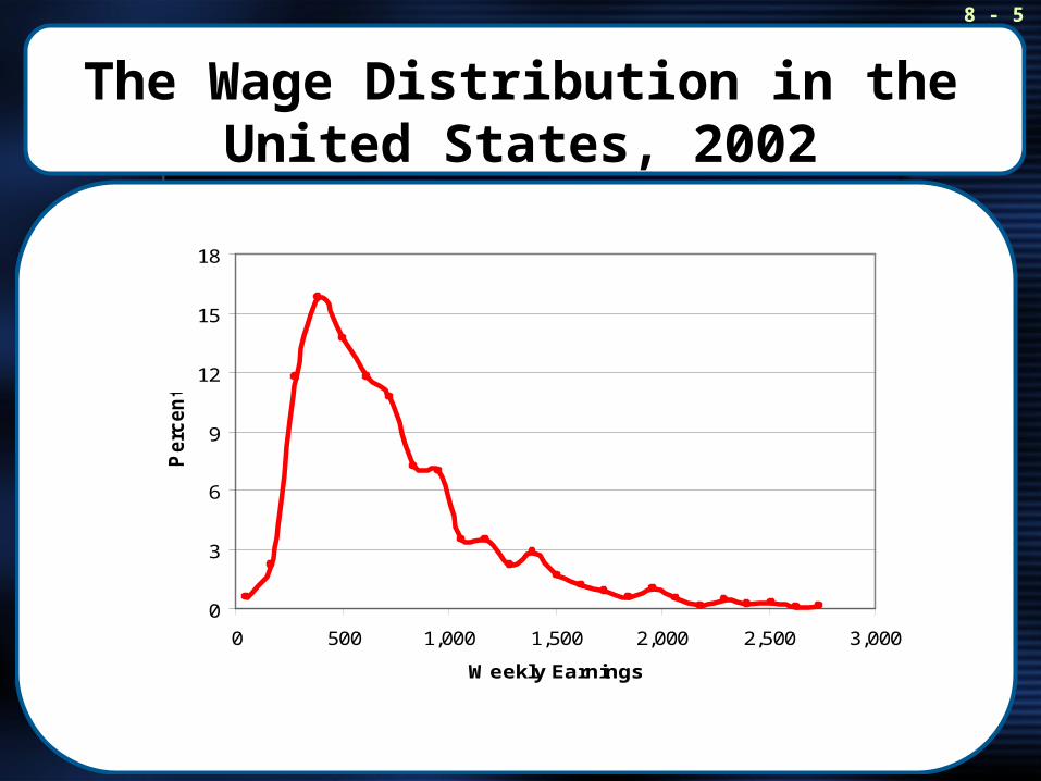
The Earnings Distribution

• The wage distribution is positively skewed (long right tail)• A small percent of workers earn disproportionately large shares

of the rewards for work

8 - 5

The Wage Distribution in the United States, 2002

0

3

6

9

12

15

18

0 500 1,000 1,500 2,000 2,500 3,000

Weekly Earnings

Perc

en

t

8 - 6

Facts About the Earnings Distribution

• Wage differentials exist due to- Human capital investments that vary from worker to worker- Age (young workers are still accumulating human capital,

older workers are collecting returns from earlier investments

• There is a positive correlation between ability and human capital investments, which “stretches out” wages in the population

8 - 7

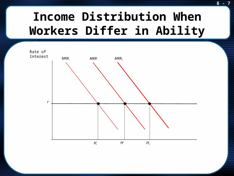
Income Distribution When Workers Differ in Ability

r

H*HLHH

Rate of Interest MRR*MRRL MRRH

8 - 8

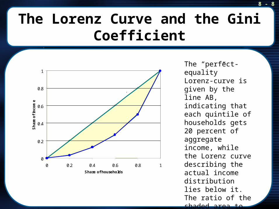
The Lorenz Curve and the Gini Coefficient

The “perfect-equality” Lorenz-curve is given by the line AB, indicating that each quintile of households gets 20 percent of aggregate income, while the Lorenz curve describing the actual income distribution lies below it. The ratio of the shaded area to the area in the triangle ABC gives the Gini coefficient.

0

0.2

0.4

0.6

0.8

1

0 0.2 0.4 0.6 0.8 1

Share of households

Sh

are

of

inco

me

A

B

C

Perfect-equalityLorenz curve

ActualLorenz curve

8 - 9

Changes in the Wage Structure – the 1980s

• The wage gap between those at the top of the wage distribution and those at the bottom widened dramatically

• Wage differentials widened among education groups, experience groups, and age groups

• Wage differentials widened within demographic and skill groups

8 - 10

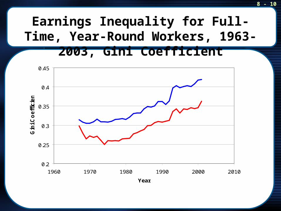
Earnings Inequality for Full-Time, Year-Round Workers, 1963-2003, Gini Coefficient

0.2

0.25

0.3

0.35

0.4

0.45

1960 1970 1980 1990 2000 2010

Year

Gin

i Co

eff

icie

nt

Men

Women

8 - 11

Earnings Inequality for Full-Time, Year-Round Workers, 1963-2003, 90-10 Wage Gap

150

200

250

300

350

400

450

1960 1970 1980 1990 2000 2010

Year

Pe

rce

nt

wa

ge

ga

p

Men

Women

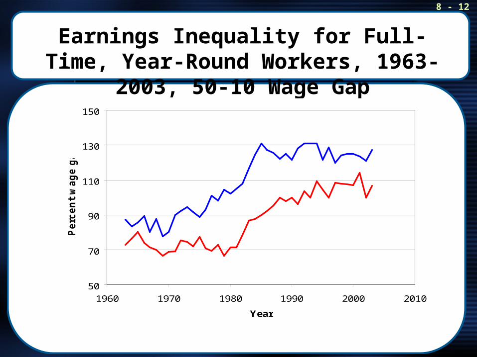
8 - 12

Earnings Inequality for Full-Time, Year-Round Workers, 1963-2003, 50-10 Wage Gap

50

70

90

110

130

150

1960 1970 1980 1990 2000 2010

Year

Pe

rce

nt

wa

ge

ga

p

Men

Women

8 - 13

Wage Differential Between College Graduates and High School Graduates, 1963-2001

40

50

60

70

80

90

100

1960 1970 1980 1990 2000 2010

Year

Pe

rce

nt

8 - 14

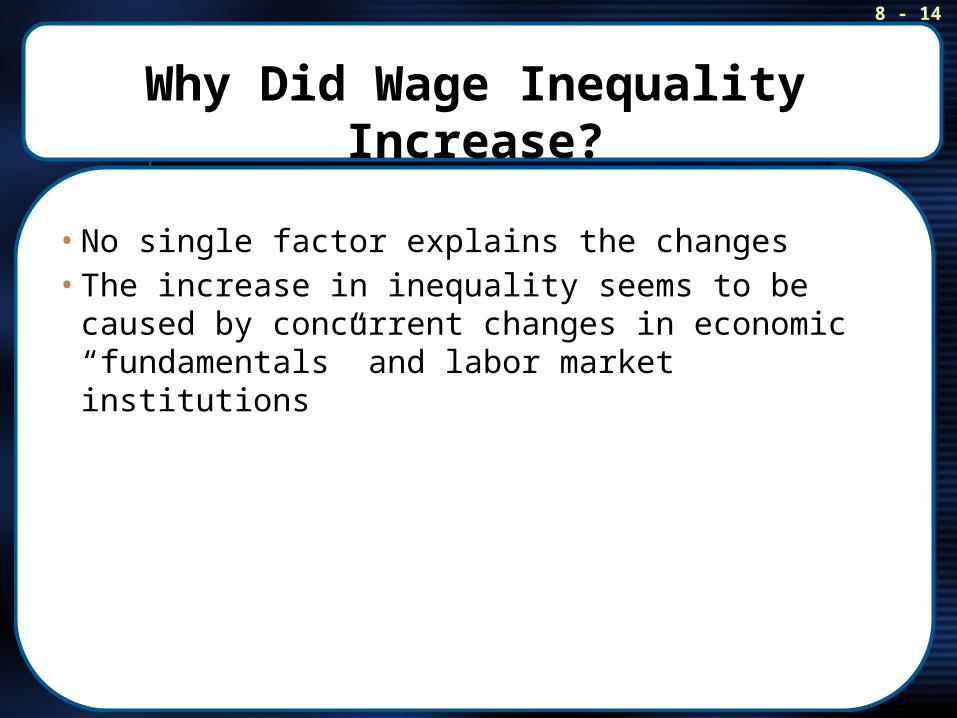
Why Did Wage Inequality Increase?

• No single factor explains the changes• The increase in inequality seems to be caused by concurrent

changes in economic “fundamentals” and labor market institutions

8 - 15

Changing the Wage Structure

• Decrease in supply of skilled workers will cause widening of wage gap

• Increase in demand for skilled workers will cause widening of wage gap

8 - 16

Possible Factors That Widened the Wage Gap

• Globalization of U.S. economy• Demand for skilled workers increased by more than the demand

increase for unskilled workers• Increased physical capital helped to increase the productivity of

skilled workers• Weakened bargaining power of unions could be from the

relative shift in demand for skilled labor

8 - 17

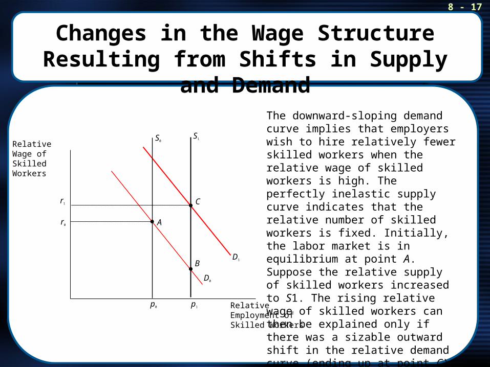
Changes in the Wage Structure Resulting from Shifts in Supply and Demand

Relative Wage of Skilled Workers

Relative Employment of Skilled Workers

A

S1S0

D0

D1

B

C

p0 p1

r0

r1

The downward-sloping demand curve implies that employers wish to hire relatively fewer skilled workers when the relative wage of skilled workers is high. The perfectly inelastic supply curve indicates that the relative number of skilled workers is fixed. Initially, the labor market is in equilibrium at point A. Suppose the relative supply of skilled workers increased to S1. The rising relative wage of skilled workers can then be explained only if there was a sizable outward shift in the relative demand curve (ending up at point C).

8 - 18

The Earnings of Superstars

• Superstar phenomenon – a few persons in some professions earn very high salaries and seem to dominate their field

• This suggests that even if a job is the same, different people bring different skills to the same job

8 - 19

Inequality Across Generations

• There is a correlation between the skills of parents and their children

• High-income parents will typically invest more in the education of their children

• There is a tendency for income differences across families to get smaller over time (“regression toward the mean”)

8 - 20

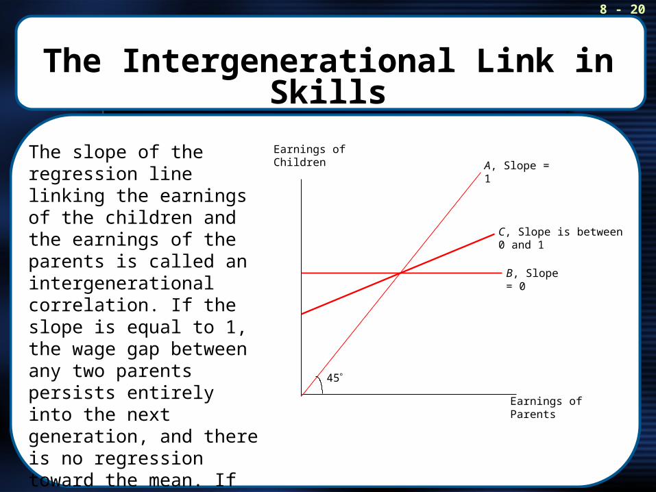
The Intergenerational Link in Skills

Earnings of Children

Earnings of Parents

45

A, Slope = 1

B, Slope = 0

C, Slope is between 0 and 1

The slope of the regression line linking the earnings of the children and the earnings of the parents is called an intergenerational correlation. If the slope is equal to 1, the wage gap between any two parents persists entirely into the next generation, and there is no regression toward the mean. If the slope is equal to 0, the wage of the children is independent of the wage of the parents, and there is complete regression toward the mean.

8 - 21

Social Capital

• The quality of the environment where a child grows up helps determine human capital

• There is evidence that varied factors influence a child’s level of human capital

- Quality of neighborhood- Importance of religious organizations- Socioeconomic background of classmates

8 - 22

End of Chapter 8