Chapter 8: Probability Density Estimationnguyen.hong.hai.free.fr/EBOOKS/SCIENCE AND... · 262...
58
Chapter 8 Probability Density Estimation 8.1 Introduction We discussed several techniques for graphical exploratory data analysis in Chapter 5. One purpose of these exploratory techniques is to obtain informa- tion and insights about the distribution of the underlying population. For instance, we would like to know if the distribution is multi-modal, skewed, symmetric, etc. Another way to gain understanding about the distribution of the data is to estimate the probability density function from the random sam- ple, possibly using a nonparametric probability density estimation tech- nique. Estimating probability density functions is required in many areas of com- putational statistics. One of these is in the modeling and simulation of phys- ical phenomena. We often have measurements from our process, and we would like to use those measurements to determine the probability distribu- tion so we can generate random variables for a Monte Carlo simulation (Chapter 6). Another application where probability density estimation is used is in statistical pattern recognition (Chapter 9). In supervised learning, which is one approach to pattern recognition, we have measurements where each one is labeled with a class membership tag. We could use the measure- ments for each class to estimate the class-conditional probability density functions, which are then used in a Bayesian classifier. In other applications, we might need to determine the probability that a random variable will fall within some interval, so we would need to evaluate the cumulative distribu- tion function. If we have an estimate of the probability density function, then we can easily estimate the required probability by integrating under the esti- mated curve. Finally, in Chapter 10, we show how to use density estimation techniques for nonparametric regression. In this chapter, we cover semi-parametric and nonparametric techniques for probability density estimation. By these, we mean techniques where we make few or no assumptions about what functional form the probability den- sity takes. This is in contrast to a parametric method, where the density is estimated by assuming a distribution and then estimating the parameters. © 2002 by Chapman & Hall/CRC
Transcript of Chapter 8: Probability Density Estimationnguyen.hong.hai.free.fr/EBOOKS/SCIENCE AND... · 262...
Chapter 8Probability Density Estimation
8.1 Introduction
We discussed several techniques for graphical exploratory data analysis inChapter 5. One purpose of these exploratory techniques is to obtain informa-tion and insights about the distribution of the underlying population. Forinstance, we would like to know if the distribution is multi-modal, skewed,symmetric, etc. Another way to gain understanding about the distribution ofthe data is to estimate the probability density function from the random sam-ple, possibly using a nonparametric probability density estimation tech-nique.
Estimating probability density functions is required in many areas of com-putational statistics. One of these is in the modeling and simulation of phys-ical phenomena. We often have measurements from our process, and wewould like to use those measurements to determine the probability distribu-tion so we can generate random variables for a Monte Carlo simulation(Chapter 6). Another application where probability density estimation isused is in statistical pattern recognition (Chapter 9). In supervised learning,which is one approach to pattern recognition, we have measurements whereeach one is labeled with a class membership tag. We could use the measure-ments for each class to estimate the class-conditional probability densityfunctions, which are then used in a Bayesian classifier. In other applications,we might need to determine the probability that a random variable will fallwithin some interval, so we would need to evaluate the cumulative distribu-tion function. If we have an estimate of the probability density function, thenwe can easily estimate the required probability by integrating under the esti-mated curve. Finally, in Chapter 10, we show how to use density estimationtechniques for nonparametric regression.
In this chapter, we cover semi-parametric and nonparametric techniquesfor probability density estimation. By these, we mean techniques where wemake few or no assumptions about what functional form the probability den-sity takes. This is in contrast to a parametric method, where the density isestimated by assuming a distribution and then estimating the parameters.
© 2002 by Chapman & Hall/CRC
260 Computational Statistics Handbook with MATLAB
We present three main methods of semi-parametric and nonparametric den-sity estimation and their variants: histograms, kernel density estimates, andfinite mixtures.
In the remainder of this section, we cover some ways to measure the errorin functions as background to what follows. Then, in Section 8.2, we presentvarious histogram based methods for probability density estimation. Therewe cover optimal bin widths for univariate and multivariate histograms, thefrequency polygons, and averaged shifted histograms. Section 8.3 contains adiscussion of kernel density estimation, both univariate and multivariate. InSection 8.4, we describe methods that model the probability density as a finite(less than n) sum of component densities. As usual, we conclude withdescriptions of available MATLAB code and references to the topics coveredin the chapter.
Before we can describe the various density estimation methods, we need toprovide a little background on measuring the error in functions. We brieflypresent two ways to measure the error between the true function and the esti-mate of the function. These are called the mean integrated squared error(MISE) and the mean integrated absolute error (MIAE). Much of the under-lying theory for choosing optimal parameters for probability density estima-tion is based on these concepts.
We start off by describing the mean squared error at a given point in thedomain of the function. We can find the mean squared error (MSE) of the esti-mate at a point x from the following
. (8.1)
Alternatively, we can determine the error over the domain for x by integrat-ing. This gives us the integrated squared error (ISE):
. (8.2)
The ISE is a random variable that depends on the true function , theestimator , and the particular random sample that was used to obtain theestimate. Therefore, it makes sense to look at the expected value of the ISE ormean integrated squared error, which is given by
. (8.3)
To obtain the mean integrated absolute error, we simply replace the inte-grand with the absolute difference between the estimate and the true func-tion. Thus, we have
f x( )
MSE f x( )[ ] E f x( ) f x( )–( )2[ ]=
ISE = f x( ) f x( )–( )2
xd∫
f x( )f x( )
MISE =E f x( ) f x( )–( )2
xd∫
© 2002 by Chapman & Hall/CRC
Chapter 8: Probability Density Estimation 261
. (8.4)
These concepts are easily extended to the multivariate case.
8.2 Histograms
Histograms were introduced in Chapter 5 as a graphical way of summarizingor describing a data set. A histogram visually conveys how a data set is dis-tributed, reveals modes and bumps, and provides information about relativefrequencies of observations. Histograms are easy to create and are computa-tionally feasible. Thus, they are well suited for summarizing large data sets.We revisit histograms here and examine optimal bin widths and where tostart the bins. We also offer several extensions of the histogram, such as thefrequency polygon and the averaged shifted histogram.
1111----D HistogD HistogD HistogD Histogrrrraaaammmmssss
Most introductory statistics textbooks expose students to the frequency his-togram and the relative frequency histogram. The problem with these is thatthe total area represented by the bins does not sum to 1. Thus, these are notvalid probability density estimates. The reader is referred to Chapter 5 formore information on this and an example illustrating the difference betweena frequency histogram and a density histogram. Since our goal is to estimatea bona fide probability density, we want to have a function that is nonne-gative and satisfies the constraint that
. (8.5)
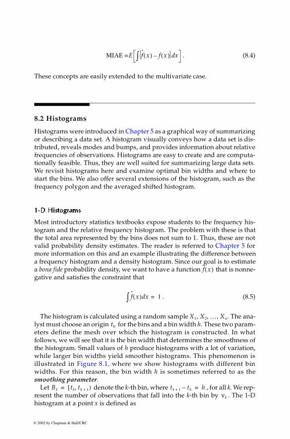
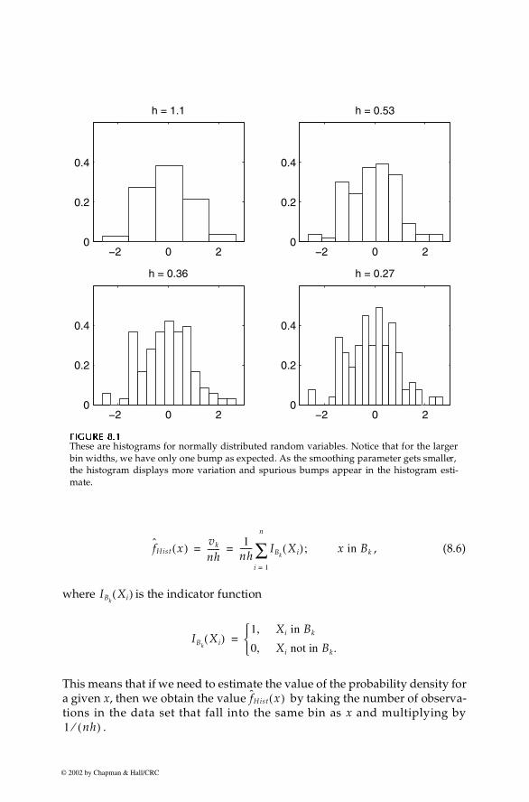
The histogram is calculated using a random sample . The ana-lyst must choose an origin for the bins and a bin width h. These two param-eters define the mesh over which the histogram is constructed. In whatfollows, we will see that it is the bin width that determines the smoothness ofthe histogram. Small values of h produce histograms with a lot of variation,while larger bin widths yield smoother histograms. This phenomenon isillustrated in Figure 8.1, where we show histograms with different binwidths. For this reason, the bin width h is sometimes referred to as thesmoothing parameter.
Let denote the k-th bin, where , for all k. We rep-resent the number of observations that fall into the k-th bin by . The 1-Dhistogram at a point x is defined as
MIAE =E f x( ) f x( )– xd∫
f x( )
f x( ) xd∫ 1=
X1 X2 … Xn, , ,t0
Bk [tk tk 1+ ),= tk 1+ tk– h=νk
© 2002 by Chapman & Hall/CRC
262 Computational Statistics Handbook with MATLAB
, (8.6)
where is the indicator function
This means that if we need to estimate the value of the probability density fora given x, then we obtain the value by taking the number of observa-tions in the data set that fall into the same bin as x and multiplying by
.
FFFFIIIIGUGUGUGURE 8.RE 8.RE 8.RE 8.1111
These are histograms for normally distributed random variables. Notice that for the largerbin widths, we have only one bump as expected. As the smoothing parameter gets smaller,the histogram displays more variation and spurious bumps appear in the histogram esti-mate.
−2 0 20
0.2
0.4
h = 1.1
−2 0 20
0.2
0.4
h = 0.53
−2 0 20
0.2
0.4
h = 0.36
−2 0 20
0.2
0.4
h = 0.27
fHist x( ) vk
nh------
1nh------ IBk
Xi( );
i 1=
n
∑= = x in Bk
IBkXi( )
IBkXi( )
1 Xi in Bk,0 Xi not in Bk.,
=
fHist x( )
1 nh( )⁄
© 2002 by Chapman & Hall/CRC
Chapter 8: Probability Density Estimation 263
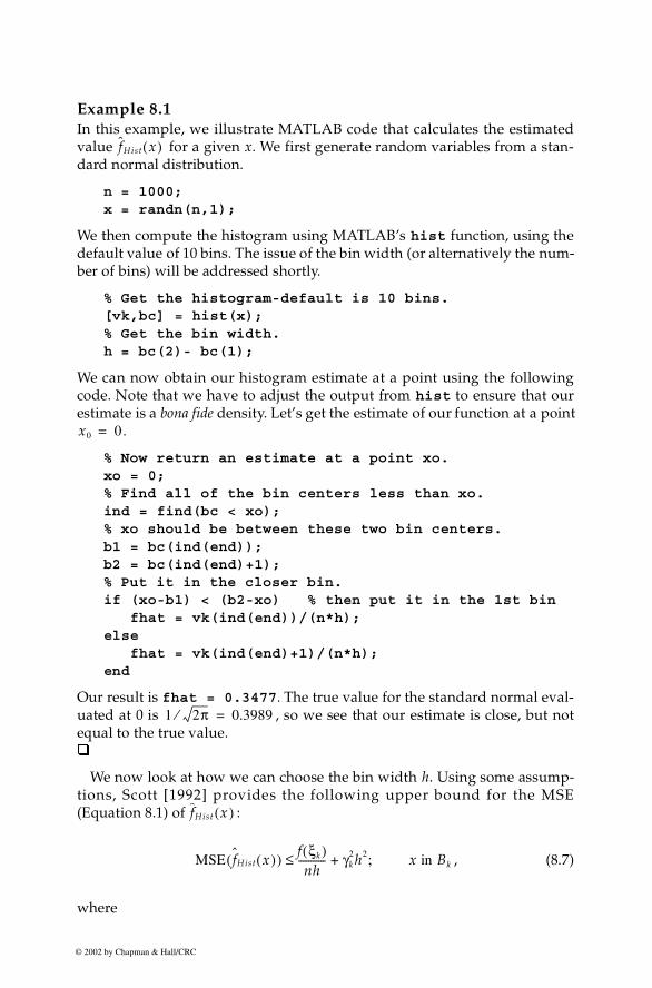
Example 8.1 In this example, we illustrate MATLAB code that calculates the estimatedvalue for a given x. We first generate random variables from a stan-dard normal distribution.
n = 1000;x = randn(n,1);
We then compute the histogram using MATLAB’s hist function, using thedefault value of 10 bins. The issue of the bin width (or alternatively the num-ber of bins) will be addressed shortly.
% Get the histogram-default is 10 bins.[vk,bc] = hist(x);% Get the bin width.h = bc(2)- bc(1);
We can now obtain our histogram estimate at a point using the followingcode. Note that we have to adjust the output from hist to ensure that ourestimate is a bona fide density. Let’s get the estimate of our function at a point
% Now return an estimate at a point xo.xo = 0;% Find all of the bin centers less than xo.ind = find(bc < xo);% xo should be between these two bin centers.b1 = bc(ind(end));b2 = bc(ind(end)+1);% Put it in the closer bin.if (xo-b1) < (b2-xo) % then put it in the 1st bin fhat = vk(ind(end))/(n*h);else fhat = vk(ind(end)+1)/(n*h);end
Our result is fhat = 0.3477. The true value for the standard normal eval-uated at 0 is , so we see that our estimate is close, but notequal to the true value.�
We now look at how we can choose the bin width h. Using some assump-tions, Scott [1992] provides the following upper bound for the MSE(Equation 8.1) of :
, (8.7)
where
fHist x( )
x0 0.=
1 2π⁄ 0.3989=
fHist x( )
MSE fHist x( )( ) f ξk( )nh
----------- γk2h2;+≤ x in Bk
© 2002 by Chapman & Hall/CRC
264 Computational Statistics Handbook with MATLAB
. (8.8)
This is based on the assumption that the probability density function isLipschitz continuous over the bin interval . A function is Lipschitz contin-uous if there is a positive constant such that
. (8.9)
The first term in Equation 8.7 is an upper bound for the variance of the den-sity estimate, and the second term is an upper bound for the squared bias ofthe density estimate. This upper bound shows what happens to the densityestimate when the bin width h is varied.
We can try to minimize the MSE by varying the bin width h. We could seth very small to reduce the bias, but this also increases the variance. Theincreased variance in our density estimate is evident in Figure 8.1, where wesee more spikes as the bin width gets smaller. Equation 8.7 shows a commonproblem in some density estimation methods: the trade-off between varianceand bias as h is changed. Most of the optimal bin widths presented here areobtained by trying to minimize the squared error.
A rule for bin width selection that is often presented in introductory statis-tics texts is called Sturges’ Rule. In reality, it is a rule that provides the numberof bins in the histogram, and is given by the following formula.
STURGES’ RULE (HISTOGRAM)
.
Here k is the number of bins. The bin width h is obtained by taking the rangeof the sample data and dividing it into the requisite number of bins, k.
Some improved values for the bin width h can be obtained by assuming theexistence of two derivatives of the probability density function . Weinclude the following results (without proof), because they are the basis formany of the univariate bin width rules presented in this chapter. The inter-ested reader is referred to Scott [1992] for more details. Most of what wepresent here follows his treatment of the subject.
Equation 8.7 provides a measure of the squared error at a point x. If wewant to measure the error in our estimate for the entire function, then we canintegrate over all values of x. Let’s assume has an absolutely continuousand a square-integrable first derivative. If we let n get very large ,then the asymptotic MISE is
hf ξk( ) f t( ) tdBk
∫ ;= for some ξk in Bk
f x( )Bk
γk
f x( ) f y( )– γk x y– ;< for all x y, in Bk
k 1 log2+ n=
f x( )
f x( )n ∞→( )
© 2002 by Chapman & Hall/CRC
Chapter 8: Probability Density Estimation 265
, (8.10)
where is used as a measure of the roughness of the function,and is the first derivative of . The first term of Equation 8.10 indicatesthe asymptotic integrated variance, and the second term refers to the asymp-totic integrated squared bias. These are obtained as approximations to theintegrated squared bias and integrated variance [Scott, 1992]. Note, however,that the form of Equation 8.10 is similar to the upper bound for the MSE inEquation 8.7 and indicates the same trade-off between bias and variance, asthe smoothing parameter h changes.
The optimal bin width for the histogram is obtained by minimizingthe AMISE (Equation 8.10), so it is the h that yields the smallest MISE as n getslarge. This is given by
. (8.11)
For the case of data that is normally distributed, we have a roughness of
.
Using this in Equation 8.11, we obtain the following expression for the opti-mal bin width for normal data.
NORMAL REFERENCE RULE - 1-D HISTOGRAM
. (8.12)
Scott [1979, 1992] proposed the sample standard deviation as an estimate of in Equation 8.12 to get the following bin width rule.
SCOTT’S RULE
.
A robust rule was developed by Freedman and Diaconis [1981]. This uses theinterquartile range (IQR) instead of the sample standard deviation.
AMISEHist h( ) 1nh------
112------h2R f ′( )+=
R g( ) g2 x( ) xd∫≡f ′ f x( )
hHist*
hHist* 6
nR f ′( )----------------
1 3⁄
=
R f ′( ) 1
4σ3 π----------------=
hHist* 24σ3 π
n-------------------
1 3⁄
= 3.5σn 1 3⁄–≈
σ
hHist*
3.5 s n 1 3⁄–××=
© 2002 by Chapman & Hall/CRC
266 Computational Statistics Handbook with MATLAB
FREEDMAN-DIACONIS RULE
.
It turns out that when the data are skewed or heavy-tailed, the bin widthsare too large using the Normal Reference Rule. Scott [1979, 1992] derived thefollowing correction factor for skewed data:
. (8.13)
The bin width obtained from Equation 8.12 should be multiplied by this fac-tor when there is evidence that the data come from a skewed distribution. Afactor for heavy-tailed distributions can be found in Scott [1992]. If one sus-pects the data come from a skewed or heavy-tailed distribution, as indicatedby calculating the corresponding sample statistics (Chapter 3) or by graphicalexploratory data analysis (Chapter 5), then the Normal Reference Rule binwidths should be multiplied by these factors. Scott [1992] shows that themodification to the bin widths is greater for skewness and is not so critical forkurtosis.
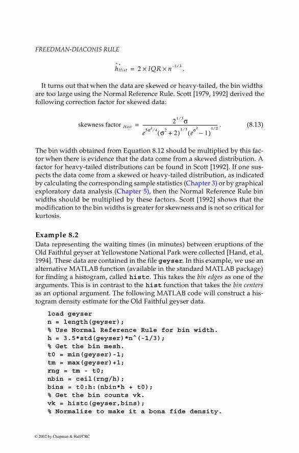
Example 8.2 Data representing the waiting times (in minutes) between eruptions of theOld Faithful geyser at Yellowstone National Park were collected [Hand, et al,1994]. These data are contained in the file geyser. In this example, we use analternative MATLAB function (available in the standard MATLAB package)for finding a histogram, called histc. This takes the bin edges as one of thearguments. This is in contrast to the hist function that takes the bin centersas an optional argument. The following MATLAB code will construct a his-togram density estimate for the Old Faithful geyser data.
load geysern = length(geyser);% Use Normal Reference Rule for bin width.h = 3.5*std(geyser)*n^(-1/3);% Get the bin mesh.t0 = min(geyser)-1;tm = max(geyser)+1;rng = tm - t0;nbin = ceil(rng/h);bins = t0:h:(nbin*h + t0);% Get the bin counts vk.vk = histc(geyser,bins);% Normalize to make it a bona fide density.
hHist*
2 IQR n 1 3⁄–××=
skewness factor Hist21 3⁄ σ
e5σ24⁄ σ2 2+( )1 3⁄
eσ2
1–( )1 2⁄
------------------------------------------------------------------=
© 2002 by Chapman & Hall/CRC
Chapter 8: Probability Density Estimation 267
% We do not need the last count in fhat.fhat(end) = [];fhat = vk/(n*h);
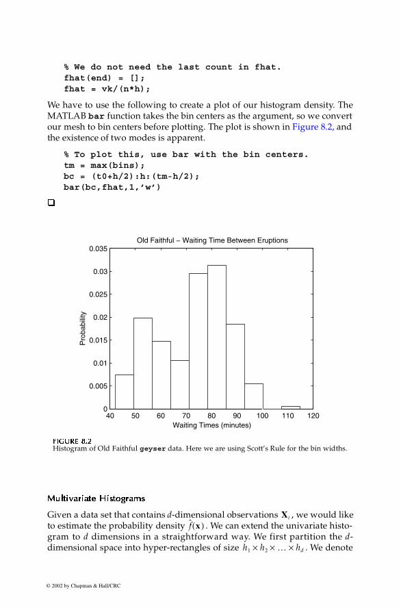
We have to use the following to create a plot of our histogram density. TheMATLAB bar function takes the bin centers as the argument, so we convertour mesh to bin centers before plotting. The plot is shown in Figure 8.2, andthe existence of two modes is apparent.
% To plot this, use bar with the bin centers.tm = max(bins);bc = (t0+h/2):h:(tm-h/2);bar(bc,fhat,1,’w’)
�
MultMultMultMultiiiivvvvarararariiiiaaaatttteeee HHHHiiiissssttttooooggggrrrraaaammmmssss
Given a data set that contains d-dimensional observations , we would liketo estimate the probability density . We can extend the univariate histo-gram to d dimensions in a straightforward way. We first partition the d-dimensional space into hyper-rectangles of size . We denote
FFFFIIIIGUGUGUGURE 8.RE 8.RE 8.RE 8.2222
Histogram of Old Faithful geyser data. Here we are using Scott’s Rule for the bin widths.
40 50 60 70 80 90 100 110 1200
0.005
0.01
0.015
0.02
0.025
0.03
0.035
Waiting Times (minutes)
Pro
babi
lity
Old Faithful − Waiting Time Between Eruptions
Xi
f x( )
h1 h2 … hd×××
© 2002 by Chapman & Hall/CRC
268 Computational Statistics Handbook with MATLAB
the k-th bin by and the number of observations falling into that bin by ,with . The multivariate histogram is then defined as
. (8.14)
If we need an estimate of the probability density at x, we first determine thebin that the observation falls into. The estimate of the probability densitywould be given by the number of observations falling into that same bindivided by the sample size and the bin widths of the partitions. The MATLABcode to create a bivariate histogram was given in Chapter 5. This could beeasily extended to the general multivariate case.
For a density function that is sufficiently smooth [Scott, 1992], we can writethe asymptotic MISE for a multivariate histogram as
, (8.15)
where As before, the first term indicates the asymptotic inte-grated variance and the second term provides the asymptotic integratedsquared bias. This has the same general form as the 1-D histogram and showsthe same bias-variance trade-off. Minimizing Equation 8.15 with respect to provides the following equation for optimal bin widths in the multivariatecase
, (8.16)
where
.
We can get a multivariate Normal Reference Rule by looking at the specialcase where the data are distributed as multivariate normal with the covari-ance equal to a diagonal matrix with along the diagonal. The Nor-mal Reference Rule in the multivariate case is given below [Scott, 1992].
Bk νk
νk∑ n=
fHist x( )νk
nh1h2…hd
--------------------------;= x in Bk
AMISEHist h( ) 1nh1h2…hd
--------------------------112------ hj
2R fj( )j 1=
d
∑+=
h h1 … hd, ,( ).=
hi
hiHist
* R fi( ) 1 2⁄– 6 R fj( )1 2⁄
j 1=
d
∏
12 d+------------
n1–
2 d+------------
=
R fi( )xi∂∂ f x( )
2
xd
ℜd
∫=
σ12 … σd
2, ,
© 2002 by Chapman & Hall/CRC
Chapter 8: Probability Density Estimation 269
NORMAL REFERENCE RULE - MULTIVARIATE HISTOGRAMS
.
Notice that this reduces to the same univariate Normal Reference Rule whend = 1. As before, we can use a suitable estimate for .
FFFFrrrreeeequenquenquenquenccccy Polygonsy Polygonsy Polygonsy Polygons
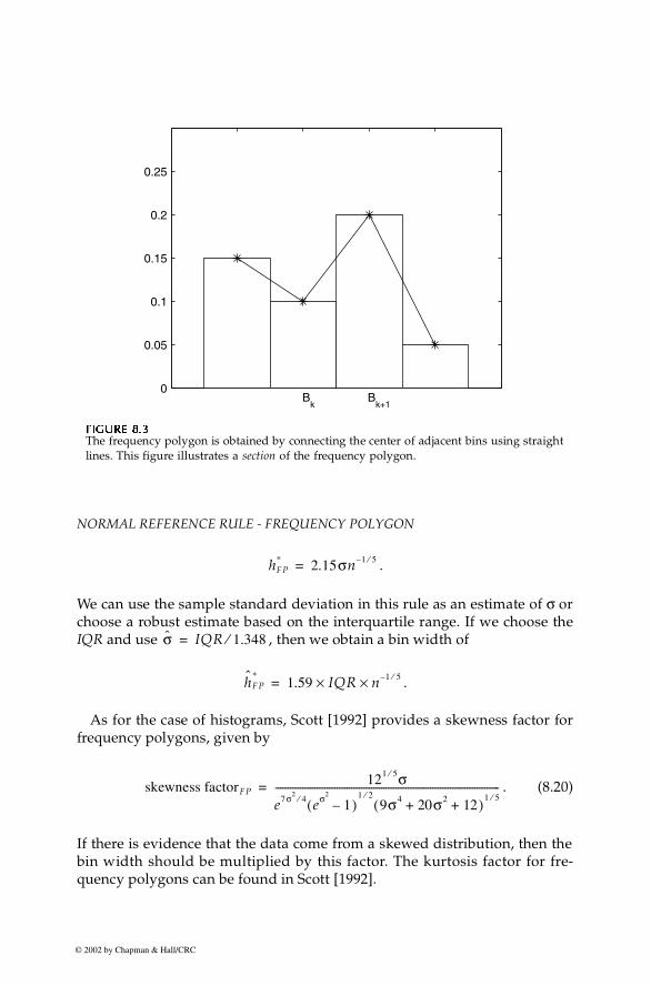
Another method for estimating probability density functions is to use a fre-quency polygon. A univariate frequency polygon approximates the densityby linearly interpolating between the bin midpoints of a histogram withequal bin widths. Because of this, the frequency polygon extends beyond thehistogram to empty bins at both ends.
The univariate probability density estimate using the frequency polygon isobtained from the following,
, (8.17)
where and are adjacent univariate histogram values and is the cen-ter of bin . An example of a section of a frequency polygon is shown in Fig-ure 8.3.
As is the case with the univariate histogram, under certain assumptions,we can write the asymptotic MISE as [Scott, 1992, 1985],
, (8.18)
where is the second derivative of . The optimal bin width that mini-mizes the AMISE for the frequency polygon is given by
. (8.19)
If is the probability density function for the standard normal, then. Substituting this in Equation 8.19, we obtain the follow-
ing Normal Reference Rule for a frequency polygon.
hiHist
* 3.5σ in1–
2 d+------------
≈ ; i 1 … d, ,=
σi
fFP x( ) 12--- x
h---–
f k12--- x
h---+
fk 1++= ; Bk x Bk 1+≤ ≤
fk fk 1+ Bk
Bk
AMISEFP h( ) 23nh----------
492880------------h4R f ″( )+=
f ″ f x( )
hFP* 2
1549nR f ″( )-----------------------
1 5⁄
=
f x( )R f ″( ) 3 8 πσ5( )⁄=
© 2002 by Chapman & Hall/CRC
270 Computational Statistics Handbook with MATLAB
NORMAL REFERENCE RULE - FREQUENCY POLYGON
.
We can use the sample standard deviation in this rule as an estimate of σ orchoose a robust estimate based on the interquartile range. If we choose theIQR and use , then we obtain a bin width of
.
As for the case of histograms, Scott [1992] provides a skewness factor forfrequency polygons, given by
. (8.20)
If there is evidence that the data come from a skewed distribution, then thebin width should be multiplied by this factor. The kurtosis factor for fre-quency polygons can be found in Scott [1992].
FFFFIIIIGUGUGUGURE 8.RE 8.RE 8.RE 8.3333
The frequency polygon is obtained by connecting the center of adjacent bins using straightlines. This figure illustrates a section of the frequency polygon.
0
0.05
0.1
0.15
0.2
0.25
Bk
Bk+1
hFP* 2.15σn 1 5⁄–=
σ IQR 1.348⁄=
hFP*
1.59 IQR× n 1 5⁄–×=
skewness factorFP121 5⁄ σ
e7σ24⁄ eσ2
1–( )1 2⁄
9σ4 20σ2 12+ +( )1 5⁄-------------------------------------------------------------------------------------------=
© 2002 by Chapman & Hall/CRC
Chapter 8: Probability Density Estimation 271
Example 8.3 Here we show how to create a frequency polygon using the Old Faithfulgeyser data. We must first create the histogram from the data, where we usethe frequency polygon Normal Reference Rule to choose the smoothingparameter.
load geysern = length(geyser);% Use Normal Reference Rule for bin width% of frequency polygon.h = 2.15*sqrt(var(geyser))*n^(-1/5);t0 = min(geyser)-1;tm = max(geyser)+1;bins = t0:h:tm;vk = histc(geyser,bins);vk(end) = [];fhat = vk/(n*h);
We then use the MATLAB function called interp1 to interpolate betweenthe bin centers. This function takes three arguments (and an optional fourthargument). The first two arguments to interp1 are the xdata and ydatavectors that contain the observed data. In our case, these are the bin centersand the bin heights from the density histogram. The third argument is a vec-tor of xinterp values for which we would like to obtain interpolatedyinterp values. There is an optional fourth argument that allows the userto select the type of interpolation (linear, cubic, nearest and spline).The default is linear, which is what we need for the frequency polygon. Thefollowing code constructs the frequency polygon for the geyser data.
% For frequency polygon, get the bin centers, % with empty bin center on each end.bc2 = (t0-h/2):h:(tm+h/2);binh = [0 fhat 0];% Use linear interpolation between bin centers% Get the interpolated values at x.xinterp = linspace(min(bc2),max(bc2));fp = interp1(bc2, binh, xinterp);
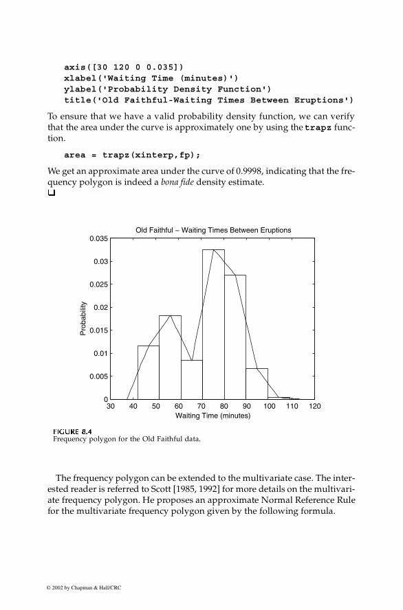
To see how this looks, we can plot the frequency polygon and underlying his-togram, which is shown in Figure 8.4.
% To plot this, use bar with the bin centerstm = max(bins);bc = (t0+h/2):h:(tm-h/2);bar(bc,fhat,1,'w')hold onplot(xinterp,fp)hold off
© 2002 by Chapman & Hall/CRC
272 Computational Statistics Handbook with MATLAB
axis([30 120 0 0.035])xlabel('Waiting Time (minutes)')ylabel('Probability Density Function')title('Old Faithful-Waiting Times Between Eruptions')
To ensure that we have a valid probability density function, we can verifythat the area under the curve is approximately one by using the trapz func-tion.
area = trapz(xinterp,fp);
We get an approximate area under the curve of 0.9998, indicating that the fre-quency polygon is indeed a bona fide density estimate.�
The frequency polygon can be extended to the multivariate case. The inter-ested reader is referred to Scott [1985, 1992] for more details on the multivari-ate frequency polygon. He proposes an approximate Normal Reference Rulefor the multivariate frequency polygon given by the following formula.
FFFFIIIIGUGUGUGURE 8.4RE 8.4RE 8.4RE 8.4
Frequency polygon for the Old Faithful data.
30 40 50 60 70 80 90 100 110 1200
0.005
0.01
0.015
0.02
0.025
0.03
0.035
Waiting Time (minutes)
Pro
babi
lity
Old Faithful − Waiting Times Between Eruptions
© 2002 by Chapman & Hall/CRC
Chapter 8: Probability Density Estimation 273
NORMAL REFERENCE RULE - FREQUENCY POLYGON (MULTIVARIATE)
,
where a suitable estimate for can be used. This is derived using theassumption that the true probability density function is multivariate normalwith covariance equal to the identity matrix. The following example illus-trates the procedure for obtaining a bivariate frequency polygon in MATLAB.
Example 8.4 We first generate some random variables that are bivariate standard normaland then calculate the surface heights corresponding to the linear interpola-tion between the histogram density bin heights.
% First get the constants.bin0 = [-4 -4];n = 1000;% Normal Reference Rule with sigma = 1. h = 3*n^(-1/4)*ones(1,2); % Generate bivariate standard normal variables.x = randn(n,2);% Find the number of bins.nb1 = ceil((max(x(:,1))-bin0(1))/h(1));nb2 = ceil((max(x(:,2))-bin0(2))/h(2));% Find the mesh or bin edges.t1 = bin0(1):h(1):(nb1*h(1)+bin0(1));t2 = bin0(2):h(2):(nb2*h(2)+bin0(2));[X,Y] = meshgrid(t1,t2);
Now that we have the random variables and the bin edges, the next step is tofind the number of observations that fall into each bin. This is easily donewith the MATLAB function inpolygon. This function can be used with anypolygon (e.g., triangle or hexagon), and it returns the indices to the pointsthat fall into that polygon.
% Find bin frequencies. [nr,nc] = size(X);vu = zeros(nr-1,nc-1);for i = 1:(nr-1)for j = 1:(nc-1)
xv = [X(i,j) X(i,j+1) X(i+1,j+1) X(i+1,j)];yv = [Y(i,j) Y(i,j+1) Y(i+1,j+1) Y(i+1,j)];in = inpolygon(x(:,1),x(:,2),xv,yv);vu(i,j) = sum(in(:));
endend
hi* 2σ in
1 4 d+( )⁄–=
σ i
© 2002 by Chapman & Hall/CRC
274 Computational Statistics Handbook with MATLAB
fhat = vu/(n*h(1)*h(2));
Now that we have the histogram density, we can use the MATLAB functioninterp2 to linearly interpolate at points between the bin centers.
% Now get the bin centers for the frequency polygon.% We add bins at the edges with zero height.t1 = (bin0(1)-h(1)/2):h(1):(max(t1)+h(1)/2);t2 = (bin0(2)-h(2)/2):h(2):(max(t2)+h(2)/2);[bcx,bcy] = meshgrid(t1,t2);[nr,nc] = size(fhat);binh = zeros(nr+2,nc+2); % add zero bin heightsbinh(2:(1+nr),2:(1+nc))=fhat;% Get points where we want to interpolate to get% the frequency polygon.[xint,yint]=meshgrid(linspace(min(t1),max(t1),30),... linspace(min(t2),max(t2),30));fp = interp2(bcx,bcy,binh,xint,yint,'linear');
We can verify that this is a valid density by estimating the area under thecurve.
df1 = xint(1,2)-xint(1,1);df2 = yint(2,1)-yint(1,1);area = sum(sum(fp))*df1*df2;
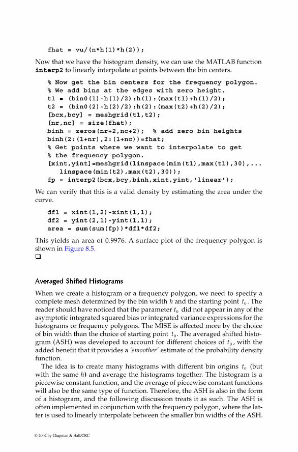
This yields an area of 0.9976. A surface plot of the frequency polygon isshown in Figure 8.5. �
AvAvAvAveeeerrrraaaaged Shifted Histogramged Shifted Histogramged Shifted Histogramged Shifted Histogramssss
When we create a histogram or a frequency polygon, we need to specify acomplete mesh determined by the bin width h and the starting point . Thereader should have noticed that the parameter did not appear in any of theasymptotic integrated squared bias or integrated variance expressions for thehistograms or frequency polygons. The MISE is affected more by the choiceof bin width than the choice of starting point . The averaged shifted histo-gram (ASH) was developed to account for different choices of , with theadded benefit that it provides a ‘smoother’ estimate of the probability densityfunction.
The idea is to create many histograms with different bin origins (butwith the same h) and average the histograms together. The histogram is apiecewise constant function, and the average of piecewise constant functionswill also be the same type of function. Therefore, the ASH is also in the formof a histogram, and the following discussion treats it as such. The ASH isoften implemented in conjunction with the frequency polygon, where the lat-ter is used to linearly interpolate between the smaller bin widths of the ASH.
t0
t0
t0
t0
t0
© 2002 by Chapman & Hall/CRC
Chapter 8: Probability Density Estimation 275
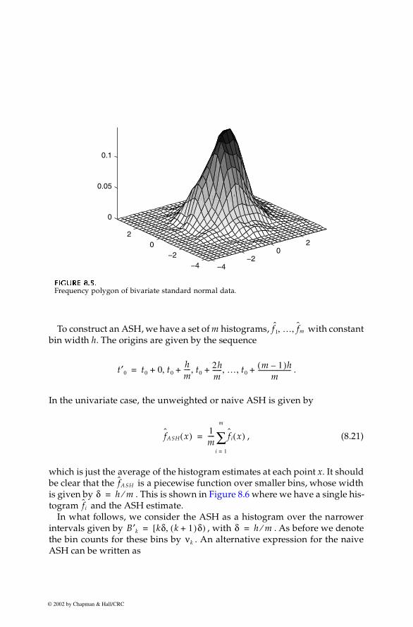
To construct an ASH, we have a set of m histograms, with constantbin width h. The origins are given by the sequence
.
In the univariate case, the unweighted or naive ASH is given by
, (8.21)
which is just the average of the histogram estimates at each point x. It shouldbe clear that the is a piecewise function over smaller bins, whose widthis given by . This is shown in Figure 8.6 where we have a single his-togram and the ASH estimate.
In what follows, we consider the ASH as a histogram over the narrowerintervals given by , with . As before we denotethe bin counts for these bins by . An alternative expression for the naiveASH can be written as
FFFFIIIIGUGUGUGURE 8.5.RE 8.5.RE 8.5.RE 8.5.
Frequency polygon of bivariate standard normal data.
−4−2
02
−4−2
02
0
0.05
0.1
f1ˆ … fm, ,
t′0 t0 0 t0hm---- t0
2hm------+ … t0
m 1–( )hm
---------------------+, , ,+,+=
fASH x( ) 1m---- f i x( )
i 1=
m
∑=
fASH
δ h m⁄=fi
B′k [kδ k 1+( )δ),= δ h m⁄=νk
© 2002 by Chapman & Hall/CRC
276 Computational Statistics Handbook with MATLAB
. (8.22)
To make this a little clearer, let’s look at a simple example of the naive ASH,with . In this case, our estimate at a point x is
We can think of the factor in Equation 8.22 as weights on the bincounts. We can use arbitrary weights instead, to obtain the general ASH.
GENERAL AVERAGED SHIFTED HISTOGRAM
. (8.23)
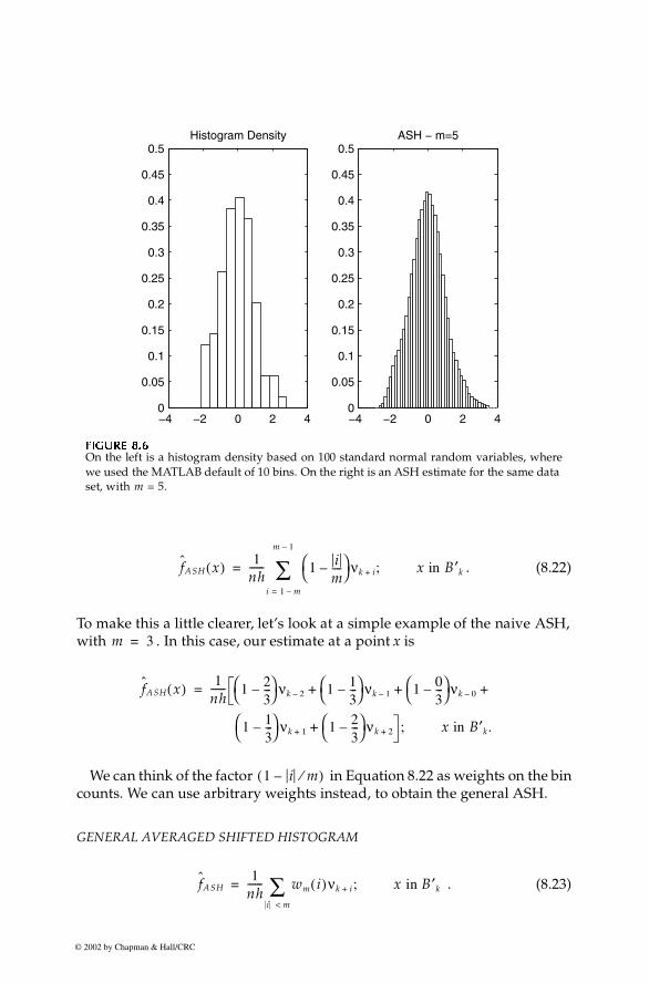
FFFFIIIIGUGUGUGURE 8.6RE 8.6RE 8.6RE 8.6
On the left is a histogram density based on 100 standard normal random variables, wherewe used the MATLAB default of 10 bins. On the right is an ASH estimate for the same dataset, with m = 5.
−4 −2 0 2 40
0.05
0.1
0.15
0.2
0.25
0.3
0.35
0.4
0.45
0.5Histogram Density
−4 −2 0 2 40
0.05
0.1
0.15
0.2
0.25
0.3
0.35
0.4
0.45
0.5ASH − m=5
fASH x( ) 1nh------ 1 i
m----–
νk i+ ;
i 1 m–=
m 1–
∑= x in B′k
m 3=
fASH x( ) 1nh------ 1 2
3---–
νk 2– 1 13---–
νk 1– 1 03---–
νk 0–
1 13---–
νk 1+ 1 23---–
νk 2+
+ + +
+ ;
=
x in B′k.
1 i m⁄–( )
fASH1
nh------ wm i( )νk i+ ;
i m<∑= x in B′k
© 2002 by Chapman & Hall/CRC
Chapter 8: Probability Density Estimation 277
A general formula for the weights is given by
, (8.24)
with K a continuous function over the interval . This function K issometimes chosen to be a probability density function. In Example 8.5, weuse the biweight function:
(8.25)
for our weights. Here is the indicator function over the interval .The algorithm for the general univariate ASH [Scott, 1992] is given here
and is also illustrated in MATLAB in Example 8.5. This algorithm requires atleast empty bins on either end.
UNIVARIATE ASH - ALGORITHM:
1. Generate a mesh over the range with bin widthsof size and . The quantity nbin is the number ofbins - see the comments below for more information on this num-ber. Include at least m - 1 empty bins on either end of the range.
2. Compute the bin counts .3. Compute the weight vector given in Equation 8.24.
4. Set all .5. Loop over to nbin
Loop over to
Calculate: .
6. Divide all by nh, these are the ASH heights.7. Calculate the bin centers using .
In practice, one usually chooses the m and h by setting the number of narrow(size ) bins between 50 and 500 over the range of the sample. This is thenextended to put some empty bins on either end of the range.
wm i( ) m K i m⁄( )
K j m⁄( )j 1 m–=
m 1–
∑----------------------------------;×= i 1 m– … m 1–, ,=
1– 1,[ ]
K t( ) 1516------ 1 t2–( )2
I 1– 1,[ ] t( )=
I 1– 1,[ ] 1– 1,[ ]
m 1–
t0 nbin δ t0+×,( )δ δ<<h, h mδ=
νk
wm i( )fk 0=
k 1=
i max 1 k m– 1+,{ }= min nbin k m 1–+,{ }
fiˆ fi
ˆ νkwm i k–( )+=
fk
Bk t0 k 0.5–( )δ+=
δ
© 2002 by Chapman & Hall/CRC
278 Computational Statistics Handbook with MATLAB
Example 8.5 In this example, we construct an ASH probability density estimate of the Buf-falo snowfall data [Scott, 1992]. These data represent the annual snowfallin inches in Buffalo, New York over the years 1910-1972. First load the dataand get the appropriate parameters.
load snowfalln = length(snowfall);m = 30;h = 14.6;delta = h/m;
The next step is to construct a mesh using the smaller bin widths of size over the desired range. Here we start the density estimate at zero.
% Get the mesh.t0 = 0;tf = max(snowfall)+20;nbin = ceil((tf-t0)/delta);binedge = t0:delta:(t0+delta*nbin);
We need to obtain the bin counts for these smaller bins, and we use the histcfunction since we want to use the bin edges rather than the bin centers.
% Get the bin counts for the smaller binwidth delta.vk = histc(snowfall,binedge);% Put into a vector with m-1 zero bins on either end.fhat = [zeros(1,m-1),vk,zeros(1,m-1)];
Next, we construct our weight vector according to Equation 8.24, where weuse the biweight kernel given in Equation 8.25. Instead of writing the kernelas a separate function, we will use the MATLAB inline function to create afunction object. We can then call that inline function just as we would anM-file function.
% Get the weight vector.% Create an inline function for the kernel.kern = inline('(15/16)*(1-x.^2).^2');ind = (1-m):(m-1);% Get the denominator. den = sum(kern(ind/m));% Create the weight vector.wm = m*(kern(ind/m))/den;
The following section of code essentially implements steps 5 - 7 of the ASHalgorithm.
% Get the bin heights over smaller bins.fhatk = zeros(1,nbin);for k = 1:nbin
δ
© 2002 by Chapman & Hall/CRC
Chapter 8: Probability Density Estimation 279
ind = k:(2*m+k-2); fhatk(k) = sum(wm.*fhat(ind));endfhatk = fhatk/(n*h);bc = t0+((1:k)-0.5)*delta;
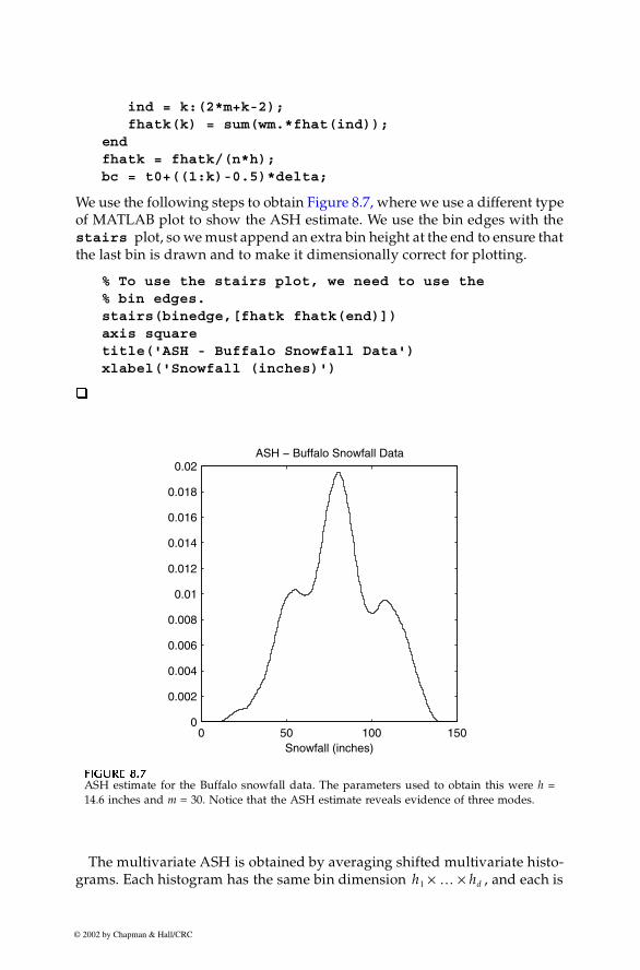
We use the following steps to obtain Figure 8.7, where we use a different typeof MATLAB plot to show the ASH estimate. We use the bin edges with thestairs plot, so we must append an extra bin height at the end to ensure thatthe last bin is drawn and to make it dimensionally correct for plotting.
% To use the stairs plot, we need to use the % bin edges.stairs(binedge,[fhatk fhatk(end)])axis squaretitle('ASH - Buffalo Snowfall Data')xlabel('Snowfall (inches)')
�
The multivariate ASH is obtained by averaging shifted multivariate histo-grams. Each histogram has the same bin dimension , and each is
FFFFIIIIGUGUGUGURE 8.7RE 8.7RE 8.7RE 8.7
ASH estimate for the Buffalo snowfall data. The parameters used to obtain this were h =14.6 inches and m = 30. Notice that the ASH estimate reveals evidence of three modes.
0 50 100 1500
0.002
0.004
0.006
0.008
0.01
0.012
0.014
0.016
0.018
0.02ASH − Buffalo Snowfall Data
Snowfall (inches)
h1 … hd××
© 2002 by Chapman & Hall/CRC
280 Computational Statistics Handbook with MATLAB
constructed using shifts along the coordinates given by multiples of Scott [1992] provides a detailed algorithm for the bivari-
ate ASH.
8.3 Kernel Density Estimation
Scott [1992] shows that as the number of histograms m approaches infinity,the ASH becomes a kernel estimate of the probability density function. Thefirst published paper describing nonparametric probability density estima-tion was by Rosenblatt [1956], where he described the general kernel estima-tor. Many papers that expanded the theory followed soon after. A partial listincludes Parzen [1962], Cencov [1962] and Cacoullos [1966]. Several refer-ences providing surveys and summaries of nonparametric density estima-tion are provided in Section 8.7. The following treatment of kernel densityestimation follows that of Silverman [1986] and Scott [1992].
UUUUnnnniiiivvvvarararariiiiaaaatttteeee KKKKeeeerrrrnnnneeeellll EEEEssssttttiiiimatormatormatormatorssss
The kernel estimator is given by
, (8.26)
where the function is called a kernel. This must satisfy the condition that to ensure that our estimate in Equation 8.26 is a bona fide density
estimate. If we define , then we can also write the kernelestimate as
. (8.27)
Usually, the kernel is a symmetric probability density function, and often astandard normal density is used. However, this does not have to be the case,and we will present other choices later in this chapter. From the definition ofa kernel density estimate, we see that our estimate inherits all of theproperties of the kernel function, such as continuity and differentiability..
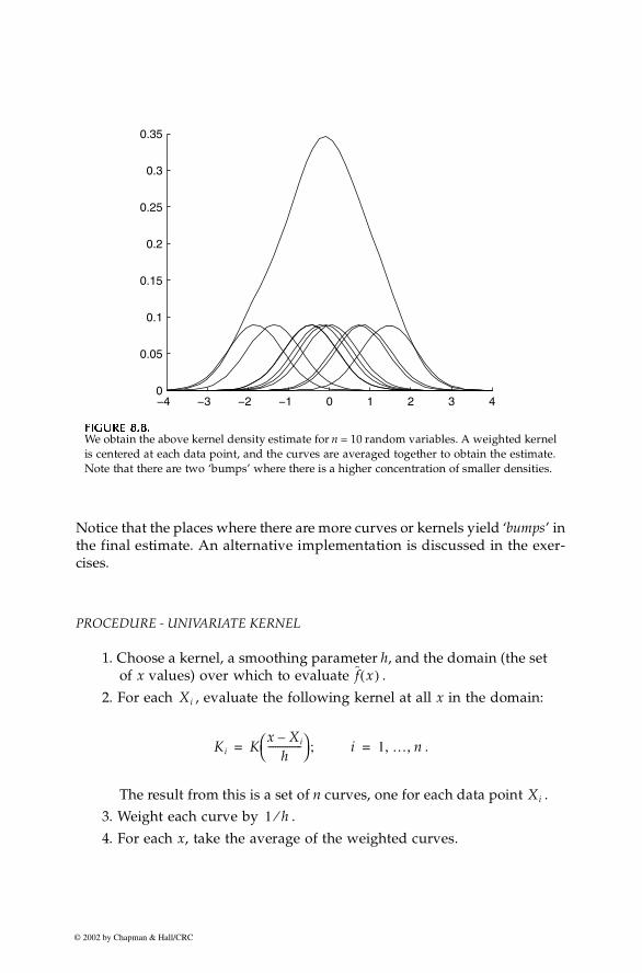
From Equation 8.26, the estimated probability density function is obtainedby placing a weighted kernel function, centered at each data point and thentaking the average of them. See Figure 8.8 for an illustration of this procedure.
δi mi⁄ i, 1 … d., ,=
fKer x( ) 1nh------ K
x Xi–h
--------------
i 1=
n
∑=
K t( )K t( ) td∫ 1=
Kh t( ) K t h⁄( ) h⁄=
fKer x( ) 1n--- Kh x Xi–( )
i 1=
n
∑=
fKer x( )
© 2002 by Chapman & Hall/CRC
Chapter 8: Probability Density Estimation 281
Notice that the places where there are more curves or kernels yield ‘bumps’ inthe final estimate. An alternative implementation is discussed in the exer-cises.
PROCEDURE - UNIVARIATE KERNEL
1. Choose a kernel, a smoothing parameter h, and the domain (the setof x values) over which to evaluate .
2. For each , evaluate the following kernel at all x in the domain:
.
The result from this is a set of n curves, one for each data point .3. Weight each curve by .
4. For each x, take the average of the weighted curves.
FFFFIIIIGUGUGUGURE 8.8.RE 8.8.RE 8.8.RE 8.8.
We obtain the above kernel density estimate for n = 10 random variables. A weighted kernelis centered at each data point, and the curves are averaged together to obtain the estimate.Note that there are two ‘bumps’ where there is a higher concentration of smaller densities.
−4 −3 −2 −1 0 1 2 3 40
0.05
0.1
0.15
0.2
0.25
0.3
0.35
f x( )Xi
Ki Kx Xi–
h--------------
;= i 1 … n, ,=
Xi
1 h⁄
© 2002 by Chapman & Hall/CRC
282 Computational Statistics Handbook with MATLAB
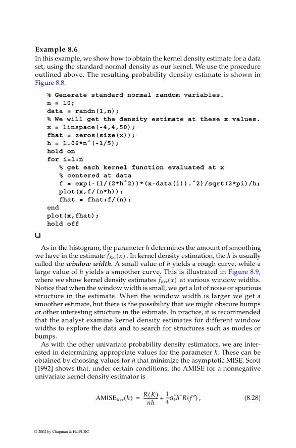
Example 8.6 In this example, we show how to obtain the kernel density estimate for a dataset, using the standard normal density as our kernel. We use the procedureoutlined above. The resulting probability density estimate is shown inFigure 8.8.
% Generate standard normal random variables.n = 10;data = randn(1,n);% We will get the density estimate at these x values.x = linspace(-4,4,50);fhat = zeros(size(x));h = 1.06*n^(-1/5);hold onfor i=1:n % get each kernel function evaluated at x
% centered at data f = exp(-(1/(2*h^2))*(x-data(i)).^2)/sqrt(2*pi)/h; plot(x,f/(n*h)); fhat = fhat+f/(n);endplot(x,fhat);hold off
�
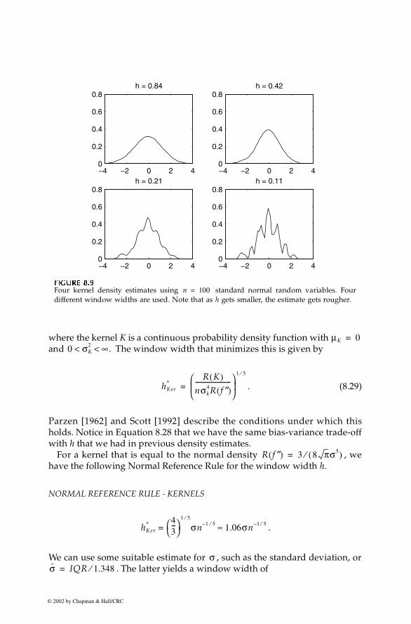
As in the histogram, the parameter h determines the amount of smoothingwe have in the estimate . In kernel density estimation, the h is usuallycalled the window width. A small value of h yields a rough curve, while alarge value of h yields a smoother curve. This is illustrated in Figure 8.9,where we show kernel density estimates at various window widths.Notice that when the window width is small, we get a lot of noise or spuriousstructure in the estimate. When the window width is larger we get asmoother estimate, but there is the possibility that we might obscure bumpsor other interesting structure in the estimate. In practice, it is recommendedthat the analyst examine kernel density estimates for different windowwidths to explore the data and to search for structures such as modes orbumps.
As with the other univariate probability density estimators, we are inter-ested in determining appropriate values for the parameter h. These can beobtained by choosing values for h that minimize the asymptotic MISE. Scott[1992] shows that, under certain conditions, the AMISE for a nonnegativeunivariate kernel density estimator is
, (8.28)
fKer x( )
fKer x( )
AMISEKer h( ) R K( )nh
-------------14---σk
4h4R f ″( )+=
© 2002 by Chapman & Hall/CRC
Chapter 8: Probability Density Estimation 283
where the kernel K is a continuous probability density function with and The window width that minimizes this is given by
. (8.29)
Parzen [1962] and Scott [1992] describe the conditions under which thisholds. Notice in Equation 8.28 that we have the same bias-variance trade-offwith h that we had in previous density estimates.
For a kernel that is equal to the normal density , wehave the following Normal Reference Rule for the window width h.
NORMAL REFERENCE RULE - KERNELS
.
We can use some suitable estimate for , such as the standard deviation, or. The latter yields a window width of
FFFFIIIIGUGUGUGURE 8.9RE 8.9RE 8.9RE 8.9
Four kernel density estimates using standard normal random variables. Fourdifferent window widths are used. Note that as h gets smaller, the estimate gets rougher.
−4 −2 0 2 40
0.2
0.4
0.6
0.8h = 0.11
−4 −2 0 2 40
0.2
0.4
0.6
0.8h = 0.21
−4 −2 0 2 40
0.2
0.4
0.6
0.8h = 0.42
−4 −2 0 2 40
0.2
0.4
0.6
0.8h = 0.84
n 100=
µK 0=0 σK
2 ∞.< <
hK er*
R K( )nσk
4R f ″( )-----------------------
1 5⁄
=
R f ″( ) 3 8 πσ5( )⁄=
hK er* 4
3---
1 5⁄
σn 1 5⁄–= 1.06σn 1 5⁄–≈
σσ IQR 1.348⁄=
© 2002 by Chapman & Hall/CRC
284 Computational Statistics Handbook with MATLAB
.
Silverman [1986] recommends that one use whichever is smaller, the samplestandard deviation or as an estimate for .
We now turn our attention to the problem of what kernel to use in our esti-mate. It is known [Scott, 1992] that the choice of smoothing parameter h ismore important than choosing the kernel. This arises from the fact that theeffects from the choice of kernel (e.g., kernel tail behavior) are reduced by theaveraging process. We discuss the efficiency of the kernels below, but whatreally drives the choice of a kernel are computational considerations or theamount of differentiability required in the estimate.
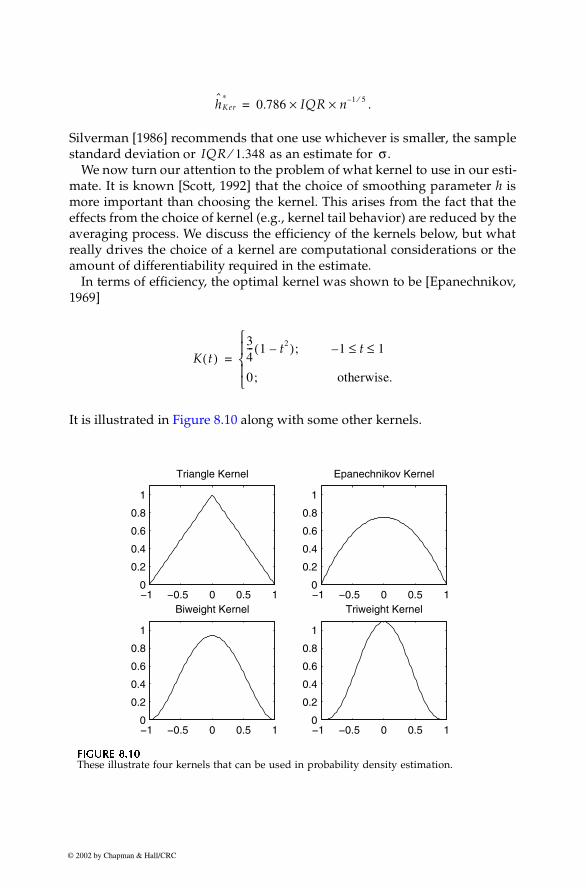
In terms of efficiency, the optimal kernel was shown to be [Epanechnikov,1969]
It is illustrated in Figure 8.10 along with some other kernels.
FFFFIIIIGUGUGUGURE 8.10RE 8.10RE 8.10RE 8.10
These illustrate four kernels that can be used in probability density estimation.
hK er*
0.786 IQR n 1 5⁄–××=
IQR 1.348⁄ σ
K t( )34--- 1 t2–( ); 1– t 1≤ ≤
0; otherwise.
=
−1 −0.5 0 0.5 10
0.2
0.4
0.6
0.8
1
Triangle Kernel
−1 −0.5 0 0.5 10
0.2
0.4
0.6
0.8
1
Epanechnikov Kernel
−1 −0.5 0 0.5 10
0.2
0.4
0.6
0.8
1
Biweight Kernel
−1 −0.5 0 0.5 10
0.2
0.4
0.6
0.8
1
Triweight Kernel
© 2002 by Chapman & Hall/CRC
Chapter 8: Probability Density Estimation 285
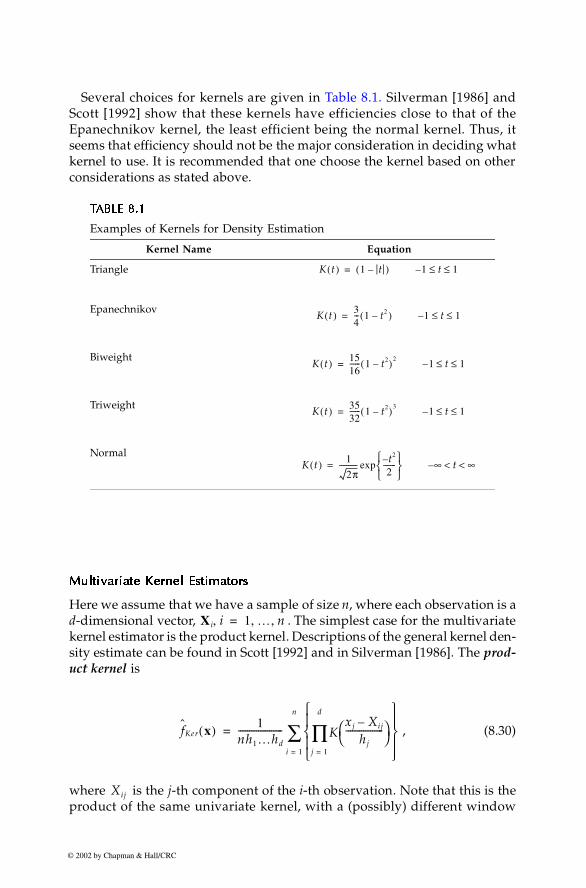
Several choices for kernels are given in Table 8.1. Silverman [1986] andScott [1992] show that these kernels have efficiencies close to that of theEpanechnikov kernel, the least efficient being the normal kernel. Thus, itseems that efficiency should not be the major consideration in deciding whatkernel to use. It is recommended that one choose the kernel based on otherconsiderations as stated above.
MultMultMultMultiiiivvvvarararariiiiaaaatttteeee KKKKeeeerrrrnnnneeeellll EEEEststststiiiimatormatormatormatorssss
Here we assume that we have a sample of size n, where each observation is ad-dimensional vector, . The simplest case for the multivariatekernel estimator is the product kernel. Descriptions of the general kernel den-sity estimate can be found in Scott [1992] and in Silverman [1986]. The prod-uct kernel is
, (8.30)
where is the j-th component of the i-th observation. Note that this is theproduct of the same univariate kernel, with a (possibly) different window
TTTTAAAABBBBLLLLE 8.1E 8.1E 8.1E 8.1
Examples of Kernels for Density Estimation
Kernel Name Equation
Triangle
Epanechnikov
Biweight
Triweight
Normal
K t( ) 1 t–( )= 1 t 1≤ ≤–
K t( ) 34--- 1 t2–( )= 1 t 1≤ ≤–
K t( ) 1516------ 1 t2–( )2
= 1 t 1≤ ≤–
K t( ) 3532------ 1 t2–( )3
= 1 t 1≤ ≤–
K t( ) 1
2π---------- t2–
2-------
exp= ∞ t ∞< <–
X i i, 1 … n, ,=
fKer x( ) 1nh1…hd
-------------------- Kxj Xij–
hj
-----------------
j 1=
d
∏
i 1=
n
∑=
Xij
© 2002 by Chapman & Hall/CRC
286 Computational Statistics Handbook with MATLAB
width in each dimension. Since the product kernel estimate is comprised ofunivariate kernels, we can use any of the kernels that were discussed previ-ously.
Scott [1992] gives expressions for the asymptotic integrated squared biasand asymptotic integrated variance for the multivariate product kernel. If thenormal kernel is used, then minimizing these yields a normal reference rulefor the multivariate case, which is given below.
NORMAL REFERENCE RULE - KERNEL (MULTIVARIATE)
,
where a suitable estimate for can be used. If there is any skewness or kur-tosis evident in the data, then the window widths should be narrower, as dis-cussed previously. The skewness factor for the frequency polygon(Equation 8.20) can be used here.
Example 8.7 In this example, we construct the product kernel estimator for the iris data.To make it easier to visualize, we use only the first two variables (sepal lengthand sepal width) for each species. So, we first create a data matrix comprisedof the first two columns for each species.
load iris% Create bivariate data matrix with all three species.data = [setosa(:,1:2)];data(51:100,:) = versicolor(:,1:2);data(101:150,:) = virginica(:,1:2);
Next we obtain the smoothing parameter using the Normal Reference Rule.
% Get the window width using the Normal Ref Rule.[n,p] = size(data);s = sqrt(var(data));hx = s(1)*n^(-1/6);hy = s(2)*n^(-1/6);
The next step is to create a grid over which we will construct the estimate.
% Get the ranges for x and y & construct grid.num_pts = 30;minx = min(data(:,1));maxx = max(data(:,1));miny = min(data(:,2));maxy = max(data(:,2));
hjK er
*4
n d 2+( )--------------------
1d 4+------------
σ j;= j 1 … d, ,=
σ j
© 2002 by Chapman & Hall/CRC
Chapter 8: Probability Density Estimation 287
gridx = ((maxx+2*hx)-(minx-2*hx))/num_ptsgridy = ((maxy+2*hy)-(miny-2*hy))/num_pts[X,Y]=meshgrid((minx-2*hx):gridx:(maxx+2*hx),...
(miny-2*hy):gridy:(maxy+2*hy));x = X(:); %put into col vectorsy = Y(:);
We are now ready to get the estimates. Note that in this example, we arechanging the form of the loop. Instead of evaluating each weighted curve andthen averaging, we will be looping over each point in the domain.
z = zeros(size(x));for i=1:length(x)
xloc = x(i)*ones(n,1);yloc = y(i)*ones(n,1);argx = ((xloc-data(:,1))/hx).^2;argy = ((yloc-data(:,2))/hy).^2;z(i) = (sum(exp(-.5*(argx+argy))))/(n*hx*hy*2*pi);
end[mm,nn] = size(X);Z = reshape(z,mm,nn);
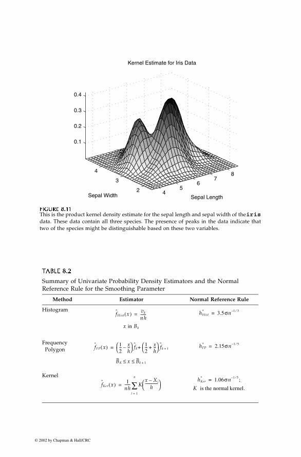
We show the surface plot for this estimate in Figure 8.11. As before, we canverify that our estimate is a bona fide by estimating the area under the curve.In this example, we get an area of 0.9994.
area = sum(sum(Z))*gridx*gridy;
�
Before leaving this section, we present a summary of univariate probabilitydensity estimators and their corresponding Normal Reference Rule for thesmoothing parameter h. These are given in Table 8.2.
8.4 Finite Mixtures
So far, we have been discussing nonparametric density estimation methodsthat require a choice of smoothing parameter h. In the previous section, weshowed that we can get different estimates of our probability densitydepending on our choice for h. It would be helpful if we could avoid choosinga smoothing parameter. In this section, we present a method called finite mix-tures that does not require a smoothing parameter. However, as is often thecase, when we eliminate one parameter we end up replacing it with another.In finite mixtures, we do not have to worry about the smoothing parameter.Instead, we have to determine the number of terms in the mixture.
© 2002 by Chapman & Hall/CRC
288 Computational Statistics Handbook with MATLAB
FFFFIIIIGUGUGUGURE 8.RE 8.RE 8.RE 8.11111111
This is the product kernel density estimate for the sepal length and sepal width of the irisdata. These data contain all three species. The presence of peaks in the data indicate thattwo of the species might be distinguishable based on these two variables.
TATATATABBBBLLLLE 8E 8E 8E 8....2222
Summary of Univariate Probability Density Estimators and the Normal Reference Rule for the Smoothing Parameter
Method Estimator Normal Reference Rule
Histogram
Frequency Polygon
Kernel
45
67
8
2
3
4
0.1
0.2
0.3
0.4
Sepal Length
Kernel Estimate for Iris Data
Sepal Width
fH ist x( ) vk
nh------=
x in Bk
hHist* 3.5σn 1 3⁄–=
fFP x( ) 12--- x
h---–
fk12--- x
h---+
fk 1++=
BK x Bk 1+≤ ≤
hFP* 2.15σn 1 5⁄–=
fKer x( ) 1nh------ K
x Xi–h
--------------
i 1=
n
∑=hKer
* 1.06σn 1 5⁄– ;=
K is the normal kernel.
© 2002 by Chapman & Hall/CRC
Chapter 8: Probability Density Estimation 289
Finite mixtures offer advantages in the area of the computational load puton the system. Two issues to consider with many probability density estima-tion methods are the computational burden in terms of the amount of infor-mation we have to store and the computational effort needed to obtain theprobability density estimate at a point. We can illustrate these ideas using thekernel density estimation method. To evaluate the estimate at a point x (in theunivariate case) we have to retain all of the data points, because the estimateis a weighted sum of n kernels centered at each sample point. In addition, wemust calculate the value of the kernel n times. The situation for histogramsand frequency polygons is a little better. The amount of information we muststore to provide an estimate of the probability density is essentially driven bythe number of bins. Of course, the situation becomes worse when we moveto multivariate kernel estimates, histograms, and frequency polygons. Withthe massive, high-dimensional data sets we often work with, the computa-tional effort and the amount of information that must be stored to use thedensity estimates is an important consideration. Finite mixtures is a tech-nique for estimating probability density functions that can require relativelylittle computer storage space or computations to evaluate the density esti-mates.
UUUUnnnniiiivvvvarararariiiiaaaatttteeee FiniFiniFiniFinitttteeee MixtuMixtuMixtuMixturrrreeeessss
The finite mixture method assumes the density can be modeled as thesum of c weighted densities, with . The most general case for theunivariate finite mixture is
, (8.31)
where represents the weight or mixing coefficient for the i-th term, and denotes a probability density, with parameters represented by the
vector To make sure that this is a bona fide density, we must impose thecondition that and To evaluate , we take ourpoint x, find the value of the component densities at that point, andtake the weighted sum of these values.
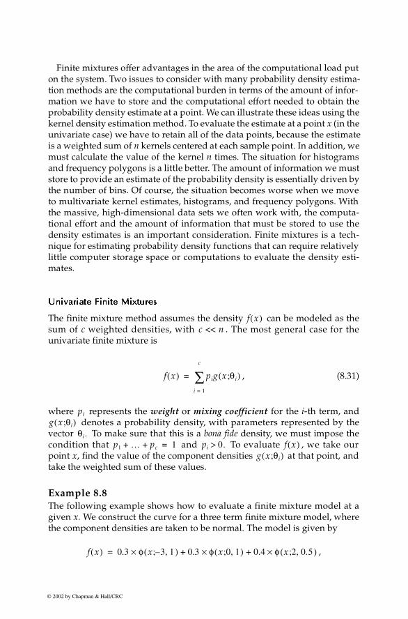
Example 8.8 The following example shows how to evaluate a finite mixture model at agiven x. We construct the curve for a three term finite mixture model, wherethe component densities are taken to be normal. The model is given by
,
f x( )c << n
f x( ) pig x θ i;( )i 1=
c
∑=
pi
g x θi;( )θi.
p1 … pc+ + 1= pi 0.> f x( )g x θi;( )
f x( ) 0.3 φ x 3 1,–;( ) 0.3 φ x 0 1,;( )× 0.4 φ x 2 0.5,;( )×+ +×=
© 2002 by Chapman & Hall/CRC
290 Computational Statistics Handbook with MATLAB
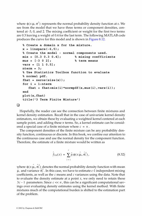
where represents the normal probability density function at x. Wesee from the model that we have three terms or component densities, cen-tered at -3, 0, and 2. The mixing coefficient or weight for the first two termsare 0.3 leaving a weight of 0.4 for the last term. The following MATLAB codeproduces the curve for this model and is shown in Figure 8.12.
% Create a domain x for the mixture.x = linspace(-6,5);% Create the model - normal components used.mix = [0.3 0.3 0.4]; % mixing coefficientsmus = [-3 0 2]; % term meansvars = [1 1 0.5];nterm = 3;% Use Statistics Toolbox function to evaluate% normal pdf.fhat = zeros(size(x));for i = 1:nterm fhat = fhat+mix(i)*normpdf(x,mus(i),vars(i));endplot(x,fhat)title('3 Term Finite Mixture')
�
Hopefully, the reader can see the connection between finite mixtures andkernel density estimation. Recall that in the case of univariate kernel densityestimators, we obtain these by evaluating a weighted kernel centered at eachsample point, and adding these n terms. So, a kernel estimate can be consid-ered a special case of a finite mixture where .
The component densities of the finite mixture can be any probability den-sity function, continuous or discrete. In this book, we confine our attention tothe continuous case and use the normal density for the component function.Therefore, the estimate of a finite mixture would be written as
, (8.32)
where denotes the normal probability density function with mean and variance . In this case, we have to estimate c-1 independent mixing
coefficients, as well as the c means and c variances using the data. Note thatto evaluate the density estimate at a point x, we only need to retain these
parameters. Since , this can be a significant computational sav-ings over evaluating density estimates using the kernel method. With finitemixtures much of the computational burden is shifted to the estimation partof the problem.
φ x µ σ2,;( )
c n=
fFM x( ) piφ x µi σ i2,;( )
i 1=
c
∑=
φ x µi σ i2
,;( )µ i σi
2
3c 1– c << n
© 2002 by Chapman & Hall/CRC
Chapter 8: Probability Density Estimation 291
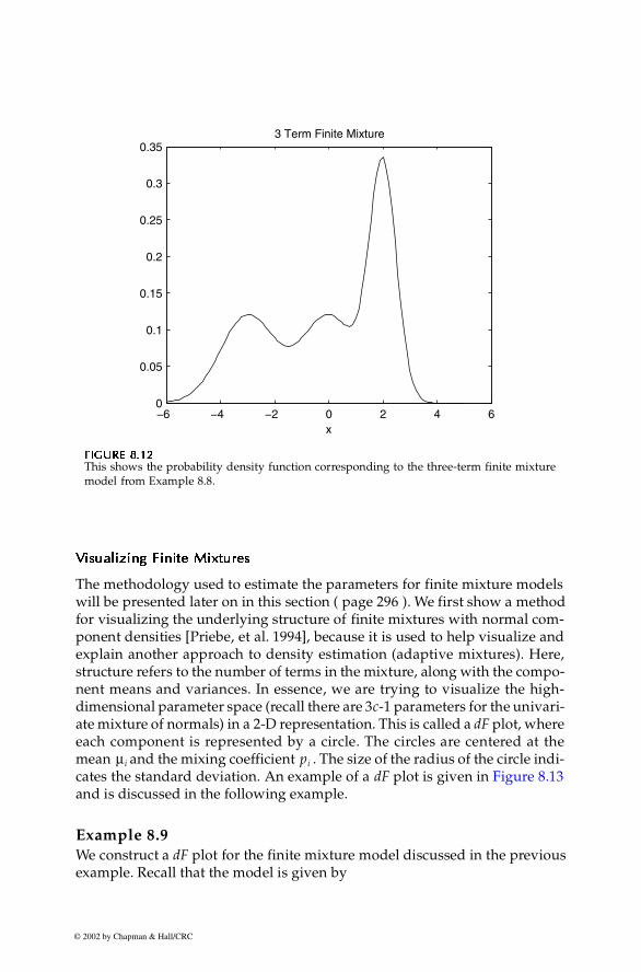
VVVVisuisuisuisuaaaalllliiiizzzziiiinnnng Finig Finig Finig Finitttteeee MixtuMixtuMixtuMixturrrreeeessss
The methodology used to estimate the parameters for finite mixture modelswill be presented later on in this section ( page 296 ). We first show a methodfor visualizing the underlying structure of finite mixtures with normal com-ponent densities [Priebe, et al. 1994], because it is used to help visualize andexplain another approach to density estimation (adaptive mixtures). Here,structure refers to the number of terms in the mixture, along with the compo-nent means and variances. In essence, we are trying to visualize the high-dimensional parameter space (recall there are 3c-1 parameters for the univari-ate mixture of normals) in a 2-D representation. This is called a dF plot, whereeach component is represented by a circle. The circles are centered at themean and the mixing coefficient . The size of the radius of the circle indi-cates the standard deviation. An example of a dF plot is given in Figure 8.13and is discussed in the following example.
Example 8.9 We construct a dF plot for the finite mixture model discussed in the previousexample. Recall that the model is given by
FFFFIIIIGUGUGUGURE 8.12RE 8.12RE 8.12RE 8.12
This shows the probability density function corresponding to the three-term finite mixturemodel from Example 8.8.
−6 −4 −2 0 2 4 60
0.05
0.1
0.15
0.2
0.25
0.3
0.353 Term Finite Mixture
x
µi pi
© 2002 by Chapman & Hall/CRC
292 Computational Statistics Handbook with MATLAB
.
Our first step is to set up the model consisting of the number of terms, thecomponent parameters and the mixing coefficients.
% Recall the model - normal components used.mix = [0.3 0.3 0.4]; % mixing coefficientsmus = [-3 0 2]; % term meansvars = [1 1 0.5];nterm = 3;
Next we set up the figure for plotting. Note that we re-scale the mixing coef-ficients for easier plotting on the vertical axis and then map the labels to thecorresponding value.
t = 0:.05:2*pi+eps; % values to create circle% To get some scales right.minx = -5;maxx = 5;scale = maxx-minx;lim = [minx maxx minx maxx];% Set up the axis limits.
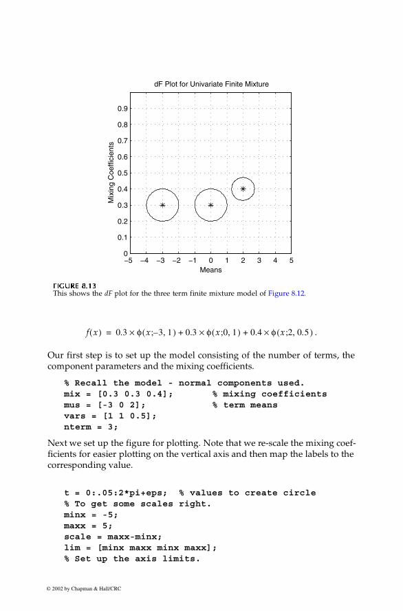
FFFFIIIIGUGUGUGURE 8.13RE 8.13RE 8.13RE 8.13
This shows the dF plot for the three term finite mixture model of Figure 8.12.
−5 −4 −3 −2 −1 0 1 2 3 4 50
0.1
0.2
0.3
0.4
0.5
0.6
0.7
0.8
0.9
Means
Mix
ing
Coe
ffici
ents
dF Plot for Univariate Finite Mixture
f x( ) 0.3 φ x 3 1,–;( ) 0.3 φ x 0 1,;( )× 0.4 φ x 2 0.5,;( )×+ +×=
© 2002 by Chapman & Hall/CRC
Chapter 8: Probability Density Estimation 293
figureaxis equalaxis(lim)grid on% Create and plot a circle for each term.hold onfor i=1:nterm % rescale for plotting purposes ycord = scale*mix(i)+minx; xc = mus(i)+sqrt(vars(i))*cos(t); yc = ycord+sqrt(vars(i))*sin(t); plot(xc,yc,mus(i),ycord,'*')endhold off% Relabel the axis to show the right coefficient.tick = (maxx-minx)/10;set(gca,'Ytick',minx:tick:maxx)set(gca,'XTick',minx:tick:maxx)set(gca,'YTickLabel',...
'0|0.1|0.2|0.3|0.4|0.5|0.6|0.7|0.8|0.9|1')xlabel('Means'),ylabel('Mixing Coefficients')title('dF Plot for Univariate Finite Mixture')
The first circle on the left corresponds to the component with and Similarly, the middle circle of Figure 8.13 represents the second
term of the model. Note that this representation of the mixture makes it easierto see which terms carry more weight and where they are located in thedomain.�
MultMultMultMultiiiivvvvarararariiiiaaaatttteeee FiniFiniFiniFinitttteeee MixtuMixtuMixtuMixturrrreeeessss
Finite mixtures is easily extended to the multivariate case. Here we define themultivariate finite mixture model as the weighted sum of multivariate com-ponent densities,
.
As before, the mixing coefficients or weights must be nonnegative and sumto one, and the component density parameters are represented by . Whenwe are estimating the function, we often use the multivariate normal as thecomponent density. This gives the following equation for an estimate of amultivariate finite mixture
pi 0.3=µ i 3.–=
f x( ) pig x; θi( )i 1=
c
∑=
θi
© 2002 by Chapman & Hall/CRC
294 Computational Statistics Handbook with MATLAB
, (8.33)
where x is a d-dimensional vector, is a d-dimensional vector of means, and is a covariance matrix. There are still c-1 mixing coefficients to esti-
mate. However, there are now values that have to be estimated for themeans and values for the component covariance matrices.
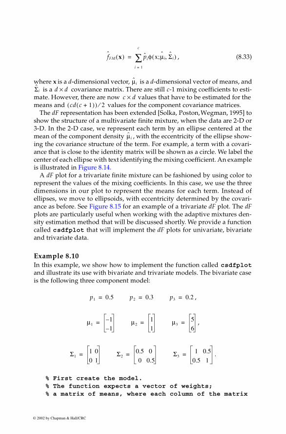
The dF representation has been extended [Solka, Poston, Wegman, 1995] toshow the structure of a multivariate finite mixture, when the data are 2-D or3-D. In the 2-D case, we represent each term by an ellipse centered at themean of the component density , with the eccentricity of the ellipse show-ing the covariance structure of the term. For example, a term with a covari-ance that is close to the identity matrix will be shown as a circle. We label thecenter of each ellipse with text identifying the mixing coefficient. An exampleis illustrated in Figure 8.14.
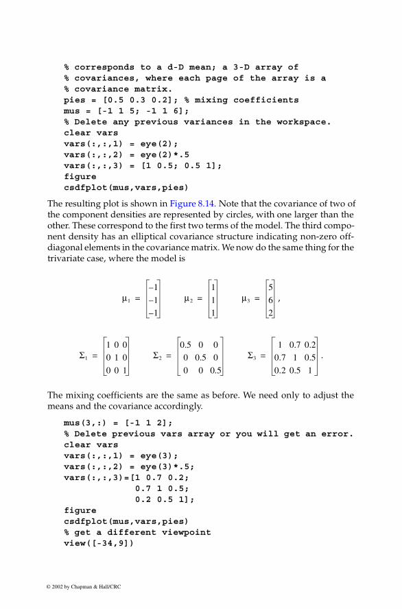
A dF plot for a trivariate finite mixture can be fashioned by using color torepresent the values of the mixing coefficients. In this case, we use the threedimensions in our plot to represent the means for each term. Instead ofellipses, we move to ellipsoids, with eccentricity determined by the covari-ance as before. See Figure 8.15 for an example of a trivariate dF plot. The dFplots are particularly useful when working with the adaptive mixtures den-sity estimation method that will be discussed shortly. We provide a functioncalled csdfplot that will implement the dF plots for univariate, bivariateand trivariate data.
Example 8.10 In this example, we show how to implement the function called csdfplotand illustrate its use with bivariate and trivariate models. The bivariate caseis the following three component model:
,
,
.
% First create the model.% The function expects a vector of weights;% a matrix of means, where each column of the matrix
fFM x( ) piφ x;µi Σ i,( )i 1=
c
∑=
µi
Σi d d×c d×
cd c 1+( )( ) 2⁄
µ i
p1 0.5= p2 0.3= p3 0.2=
µ11–
1–= µ2
1
1= µ3
5
6=
Σ11 0
0 1= Σ2
0.5 0
0 0.5= Σ3
1 0.5
0.5 1=
© 2002 by Chapman & Hall/CRC
Chapter 8: Probability Density Estimation 295
% corresponds to a d-D mean; a 3-D array of % covariances, where each page of the array is a% covariance matrix.pies = [0.5 0.3 0.2]; % mixing coefficientsmus = [-1 1 5; -1 1 6];% Delete any previous variances in the workspace.clear varsvars(:,:,1) = eye(2); vars(:,:,2) = eye(2)*.5vars(:,:,3) = [1 0.5; 0.5 1];figurecsdfplot(mus,vars,pies)
The resulting plot is shown in Figure 8.14. Note that the covariance of two ofthe component densities are represented by circles, with one larger than theother. These correspond to the first two terms of the model. The third compo-nent density has an elliptical covariance structure indicating non-zero off-diagonal elements in the covariance matrix. We now do the same thing for thetrivariate case, where the model is
,
.
The mixing coefficients are the same as before. We need only to adjust themeans and the covariance accordingly.
mus(3,:) = [-1 1 2];% Delete previous vars array or you will get an error.clear varsvars(:,:,1) = eye(3);vars(:,:,2) = eye(3)*.5;vars(:,:,3)=[1 0.7 0.2; 0.7 1 0.5; 0.2 0.5 1];figurecsdfplot(mus,vars,pies)% get a different viewpointview([-34,9])
µ1
1–
1–
1–
= µ2
1
1
1
= µ3
5
6
2
=
Σ1
1 0 0
0 1 0
0 0 1
= Σ2
0.5 0 0
0 0.5 0
0 0 0.5
= Σ3
1 0.7 0.2
0.7 1 0.5
0.2 0.5 1
=
© 2002 by Chapman & Hall/CRC
296 Computational Statistics Handbook with MATLAB
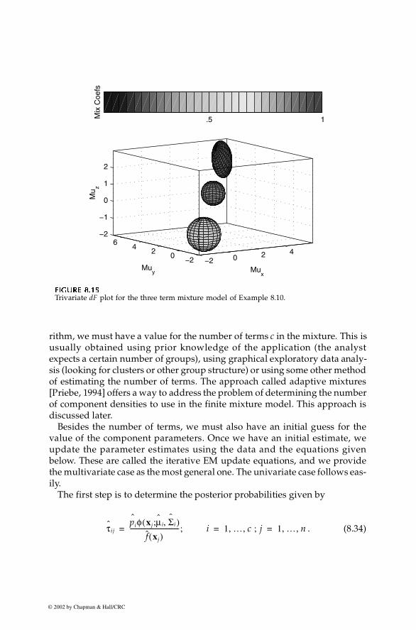
The trivariate dF plot for this model is shown in Figure 8.15. Two terms (thefirst two) are shown as spheres and one as an ellipsoid.�
EEEEM AM AM AM Allllggggoooorrrrithm forithm forithm forithm for EEEEstistististimmmmaaaattttinininingggg ththththeeee PPPPaaaarrrraaaammmmeeeetttteeeerrrrssss
The problem of estimating the parameters in a finite mixture has been stud-ied extensively in the literature. The book by Everitt and Hand [1981] pro-vides an excellent overview of this topic and offers several methods forparameter estimation. The technique we present here is called the Expecta-tion-Maximization (EM) method. This is a general method for optimizinglikelihood functions and is useful in situations where data might be missingor simpler optimization methods fail. The seminal paper on this topic is byDempster, Laird and Rubin [1977], where they formalize the EM algorithmand establish its properties. Redner and Walker [1984] apply it to mixturedensities. The EM methodology is now a standard tool for statisticians and isused in many applications.
In this section, we discuss the EM algorithm as it can be applied to estimat-ing the parameters of a finite mixture of normal densities. To use the EM algo-
FFFFIIIIGUGUGUGURE 8.14RE 8.14RE 8.14RE 8.14
Bivariate dF plot for the three term mixture model of Example 8.10.
−3 −2 −1 0 1 2 3 4 5 6 7
−1
0
1
2
3
4
5
6
0.5
0.3
0.2
µx
µ y
dF Plot
© 2002 by Chapman & Hall/CRC
Chapter 8: Probability Density Estimation 297
rithm, we must have a value for the number of terms c in the mixture. This isusually obtained using prior knowledge of the application (the analystexpects a certain number of groups), using graphical exploratory data analy-sis (looking for clusters or other group structure) or using some other methodof estimating the number of terms. The approach called adaptive mixtures[Priebe, 1994] offers a way to address the problem of determining the numberof component densities to use in the finite mixture model. This approach isdiscussed later.
Besides the number of terms, we must also have an initial guess for thevalue of the component parameters. Once we have an initial estimate, weupdate the parameter estimates using the data and the equations givenbelow. These are called the iterative EM update equations, and we providethe multivariate case as the most general one. The univariate case follows eas-ily.
The first step is to determine the posterior probabilities given by
. (8.34)
FFFFIIIIGUGUGUGURE 8.15RE 8.15RE 8.15RE 8.15
Trivariate dF plot for the three term mixture model of Example 8.10.
.5 1Mix
Coe
fs
−2 0 2 4−2
02
46
−2
−1
0
1
2
Mux
Muy
Mu z
τijpiˆ φ xj µ i Σˆ i,;( )
f xj( )-------------------------------;= i 1 … c ; j, , 1 … n, ,= =
© 2002 by Chapman & Hall/CRC
298 Computational Statistics Handbook with MATLAB
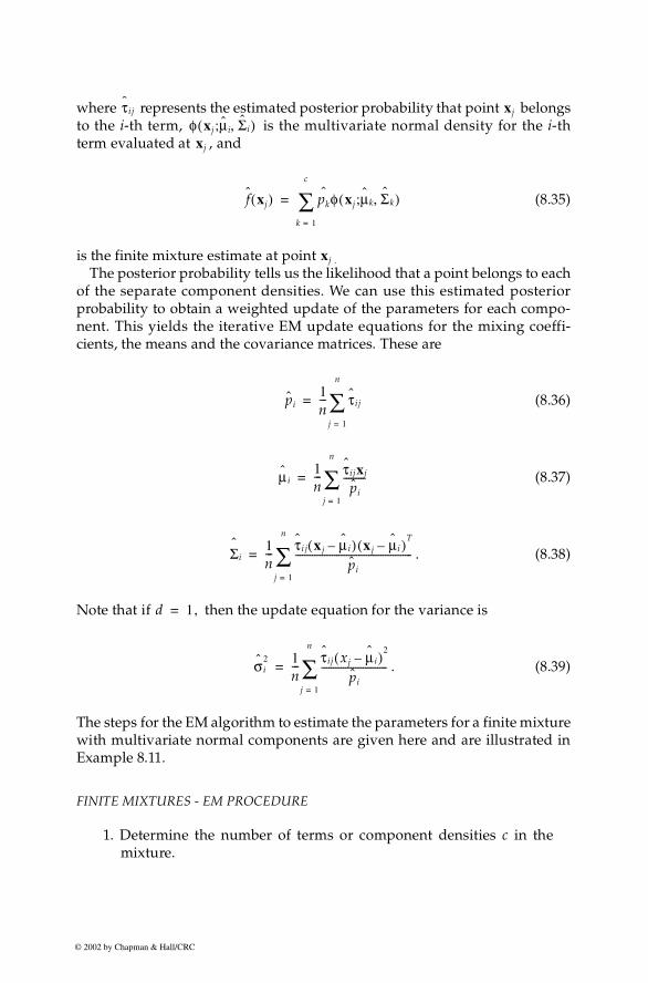
where represents the estimated posterior probability that point belongsto the i-th term, is the multivariate normal density for the i-thterm evaluated at , and
(8.35)
is the finite mixture estimate at point .
The posterior probability tells us the likelihood that a point belongs to eachof the separate component densities. We can use this estimated posteriorprobability to obtain a weighted update of the parameters for each compo-nent. This yields the iterative EM update equations for the mixing coeffi-cients, the means and the covariance matrices. These are
(8.36)
(8.37)
. (8.38)
Note that if then the update equation for the variance is
. (8.39)
The steps for the EM algorithm to estimate the parameters for a finite mixturewith multivariate normal components are given here and are illustrated inExample 8.11.
FINITE MIXTURES - EM PROCEDURE
1. Determine the number of terms or component densities c in themixture.
τij xj
φ xj µi Σi,;( )xj
f xj( ) pkˆ φ xj µk Σk,;( )
k 1=
c
∑=
xj
pi1n--- τij
j 1=
n
∑=
µ i1n--- τijxj
pi
---------
j 1=
n
∑=
Σˆ
i1n--- τi j x j µ i–( ) x j µi–( )T
pi
------------------------------------------------
j 1=
n
∑=
d 1,=
σ i2 1
n--- τij xj µ i–( )
2
pi
---------------------------
j 1=
n
∑=
© 2002 by Chapman & Hall/CRC
Chapter 8: Probability Density Estimation 299
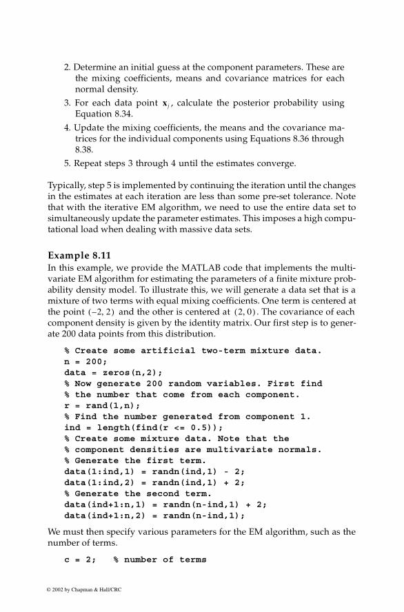
2. Determine an initial guess at the component parameters. These arethe mixing coefficients, means and covariance matrices for eachnormal density.
3. For each data point , calculate the posterior probability usingEquation 8.34.
4. Update the mixing coefficients, the means and the covariance ma-trices for the individual components using Equations 8.36 through8.38.
5. Repeat steps 3 through 4 until the estimates converge.
Typically, step 5 is implemented by continuing the iteration until the changesin the estimates at each iteration are less than some pre-set tolerance. Notethat with the iterative EM algorithm, we need to use the entire data set tosimultaneously update the parameter estimates. This imposes a high compu-tational load when dealing with massive data sets.
Example 8.11 In this example, we provide the MATLAB code that implements the multi-variate EM algorithm for estimating the parameters of a finite mixture prob-ability density model. To illustrate this, we will generate a data set that is amixture of two terms with equal mixing coefficients. One term is centered atthe point and the other is centered at . The covariance of eachcomponent density is given by the identity matrix. Our first step is to gener-ate 200 data points from this distribution.
% Create some artificial two-term mixture data.n = 200;data = zeros(n,2);% Now generate 200 random variables. First find% the number that come from each component.r = rand(1,n);% Find the number generated from component 1.ind = length(find(r <= 0.5));% Create some mixture data. Note that the % component densities are multivariate normals.% Generate the first term.data(1:ind,1) = randn(ind,1) - 2;data(1:ind,2) = randn(ind,1) + 2;% Generate the second term.data(ind+1:n,1) = randn(n-ind,1) + 2;data(ind+1:n,2) = randn(n-ind,1);
We must then specify various parameters for the EM algorithm, such as thenumber of terms.
c = 2; % number of terms
x j
2– 2,( ) 2 0,( )
© 2002 by Chapman & Hall/CRC
300 Computational Statistics Handbook with MATLAB
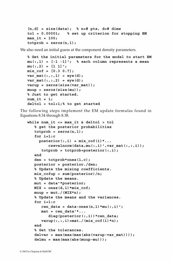
[n,d] = size(data); % n=# pts, d=# dimstol = 0.00001; % set up criterion for stopping EMmax_it = 100;totprob = zeros(n,1);
We also need an initial guess at the component density parameters.
% Get the initial parameters for the model to start EMmu(:,1) = [-1 -1]'; % each column represents a meanmu(:,2) = [1 1]';mix_cof = [0.3 0.7];var_mat(:,:,1) = eye(d);var_mat(:,:,2) = eye(d);varup = zeros(size(var_mat));muup = zeros(size(mu));% Just to get started.num_it = 1;deltol = tol+1;% to get started
The following steps implement the EM update formulas found inEquations 8.34 through 8.38.
while num_it <= max_it & deltol > tol % get the posterior probabilities totprob = zeros(n,1);
for i=1:c posterior(:,i) = mix_cof(i)*...
csevalnorm(data,mu(:,i)',var_mat(:,:,i)); totprob = totprob+posterior(:,i); end den = totprob*ones(1,c); posterior = posterior./den; % Update the mixing coefficients. mix_cofup = sum(posterior)/n; % Update the means. mut = data'*posterior; MIX = ones(d,1)*mix_cof; muup = mut./(MIX*n); % Update the means and the variances. for i=1:c cen_data = data-ones(n,1)*mu(:,i)'; mat = cen_data'*... diag(posterior(:,i))*cen_data; varup(:,:,i)=mat./(mix_cof(i)*n); end % Get the tolerances.
delvar = max(max(max(abs(varup-var_mat))));delmu = max(max(abs(muup-mu)));
© 2002 by Chapman & Hall/CRC
Chapter 8: Probability Density Estimation 301
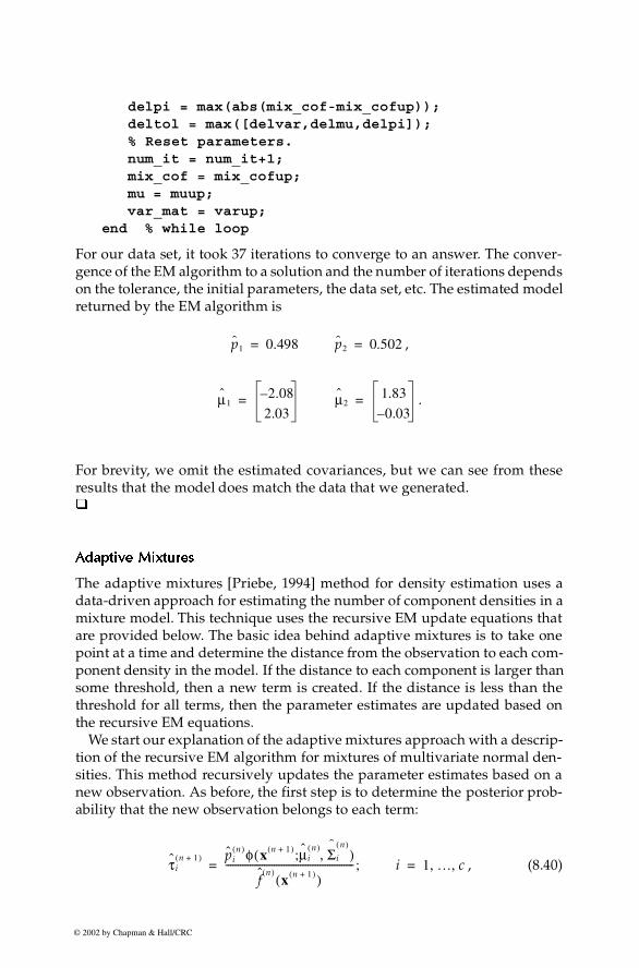
delpi = max(abs(mix_cof-mix_cofup));deltol = max([delvar,delmu,delpi]);% Reset parameters.num_it = num_it+1;mix_cof = mix_cofup;mu = muup;
var_mat = varup;end % while loop
For our data set, it took 37 iterations to converge to an answer. The conver-gence of the EM algorithm to a solution and the number of iterations dependson the tolerance, the initial parameters, the data set, etc. The estimated modelreturned by the EM algorithm is
,
.
For brevity, we omit the estimated covariances, but we can see from theseresults that the model does match the data that we generated.�
AdaptivAdaptivAdaptivAdaptiveeee MixtuMixtuMixtuMixturrrreeeessss
The adaptive mixtures [Priebe, 1994] method for density estimation uses adata-driven approach for estimating the number of component densities in amixture model. This technique uses the recursive EM update equations thatare provided below. The basic idea behind adaptive mixtures is to take onepoint at a time and determine the distance from the observation to each com-ponent density in the model. If the distance to each component is larger thansome threshold, then a new term is created. If the distance is less than thethreshold for all terms, then the parameter estimates are updated based onthe recursive EM equations.
We start our explanation of the adaptive mixtures approach with a descrip-tion of the recursive EM algorithm for mixtures of multivariate normal den-sities. This method recursively updates the parameter estimates based on anew observation. As before, the first step is to determine the posterior prob-ability that the new observation belongs to each term:
, (8.40)
p1 0.498= p2 0.502=
µ12.08–
2.03= µ2
1.83
0.03–=
τin 1+( ) pi
n( )φ x n 1+( ) µin( ) Σ
ˆi
n( ),;( )
fn( )
x n 1+( )( )-----------------------------------------------------;= i 1 … c, ,=
© 2002 by Chapman & Hall/CRC
302 Computational Statistics Handbook with MATLAB
where represents the estimated posterior probability that the newobservation belongs to the i-th term, and the superscript denotesthe estimated parameter values based on the previous n observations. Thedenominator is the finite mixture density estimate
for the new observation using the mixture from the previous n points.The remainder of the recursive EM update equations are given by Equa-
tions 8.41 through 8.43. Note that recursive equations are typically in theform of the old value for an estimate plus an update term using the newobservation. The recursive update equations for mixtures of multivariatenormals are:
(8.41)
(8.42)
. (8.43)
This reduces to the 1-D case in a straightforward manner, as was the case withthe iterative EM update equations.
The adaptive mixtures approach updates our probability density estimate and also provides the opportunity to expand the parameter space (i.e.,
the model) if the data indicate that should be done. To accomplish this, weneed a way to determine when a new component density should be added.This could be done in several ways, but the one we present here is based onthe Mahalanobis distance. If this distance is too large for all of the terms (oralternatively if the minimum distance is larger than some threshold), then wecan consider the new point too far away from the existing terms to update thecurrent model. Therefore, we create a new term.
The squared Mahalanobis distance between the new observation and the i-th term is given by
. (8.44)
We create a new term if
τin 1+( )
x n 1+( ) n( )
fn( )
x n 1+( )( ) piφ x n 1+( ); µin( ) Σ i
n( ),( )i 1=
c
∑=
pin 1+( ) pi
n( ) 1n--- τi
n 1+( )pi
n( )–( )+=
µ in 1+( ) µi
n( ) τin 1+( )
npin( )
------------- x n 1+( ) µin( )
–( )+=
Σˆ
i
n 1+( )Σˆ
i
n( ) τin 1+( )
npin( )
------------- x n 1+( ) µ in( )
–( ) x n 1+( ) µin( )
–( )T
Σ in( )
–+=
f x( )
x n 1+( )
MDi2 x n 1+( )( ) x n 1+( ) µi
n( )–( )
TΣi
n( )
1–
x n 1+( ) µin( )
–( )=
© 2002 by Chapman & Hall/CRC
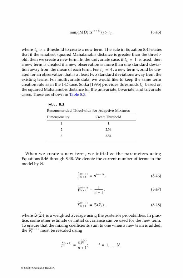
Chapter 8: Probability Density Estimation 303
, (8.45)
where is a threshold to create a new term. The rule in Equation 8.45 statesthat if the smallest squared Mahalanobis distance is greater than the thresh-old, then we create a new term. In the univariate case, if is used, thena new term is created if a new observation is more than one standard devia-tion away from the mean of each term. For , a new term would be cre-ated for an observation that is at least two standard deviations away from theexisting terms. For multivariate data, we would like to keep the same termcreation rate as in the 1-D case. Solka [1995] provides thresholds based onthe squared Mahalanobis distance for the univariate, bivariate, and trivariatecases. These are shown in Table 8.3.
When we create a new term, we initialize the parameters usingEquations 8.46 through 8.48. We denote the current number of terms in themodel by N.
, (8.46)
, (8.47)
, (8.48)
where is a weighted average using the posterior probabilities. In prac-tice, some other estimate or initial covariance can be used for the new term.To ensure that the mixing coefficients sum to one when a new term is added,the must be rescaled using
.
TTTTAAAABBBBLLLLEEEE 8888.3.3.3.3
Recommended Thresholds for Adaptive Mixtures
Dimensionality Create Threshold
1 1
2 2.34
3 3.54
min i MDi2 x n 1+( )( ){ } tC>
tC
tC 1=
tC 4=
tC
µN 1+n 1+( )
x n 1+( )=
pN 1+n 1+( ) 1
n 1+------------=
ΣN 1+n 1+( ) ℑ Σi( )=
ℑ Σi( )
pin 1+( )
pin 1+( ) npi
n( )
n 1+------------ ;= i 1 … N, ,=
© 2002 by Chapman & Hall/CRC
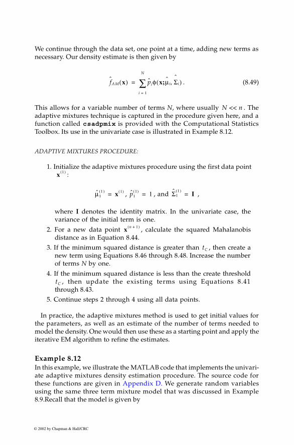
304 Computational Statistics Handbook with MATLAB
We continue through the data set, one point at a time, adding new terms asnecessary. Our density estimate is then given by
. (8.49)
This allows for a variable number of terms N, where usually . Theadaptive mixtures technique is captured in the procedure given here, and afunction called csadpmix is provided with the Computational StatisticsToolbox. Its use in the univariate case is illustrated in Example 8.12.
ADAPTIVE MIXTURES PROCEDURE:
1. Initialize the adaptive mixtures procedure using the first data point:
, , and ,
where I denotes the identity matrix. In the univariate case, thevariance of the initial term is one.
2. For a new data point , calculate the squared Mahalanobisdistance as in Equation 8.44.
3. If the minimum squared distance is greater than , then create anew term using Equations 8.46 through 8.48. Increase the numberof terms N by one.
4. If the minimum squared distance is less than the create threshold, then update the existing terms using Equations 8.41
through 8.43.5. Continue steps 2 through 4 using all data points.
In practice, the adaptive mixtures method is used to get initial values forthe parameters, as well as an estimate of the number of terms needed tomodel the density. One would then use these as a starting point and apply theiterative EM algorithm to refine the estimates.
Example 8.12 In this example, we illustrate the MATLAB code that implements the univari-ate adaptive mixtures density estimation procedure. The source code forthese functions are given in Appendix D. We generate random variablesusing the same three term mixture model that was discussed in Example8.9.Recall that the model is given by
fAM x( ) piφ x;µ i Σˆ
i,( )i 1=
N
∑=
N << n
x 1( )
µ11( ) x 1( )= p1
1( ) 1= Σ11( )
I=
x n 1+( )
tC
tC
© 2002 by Chapman & Hall/CRC
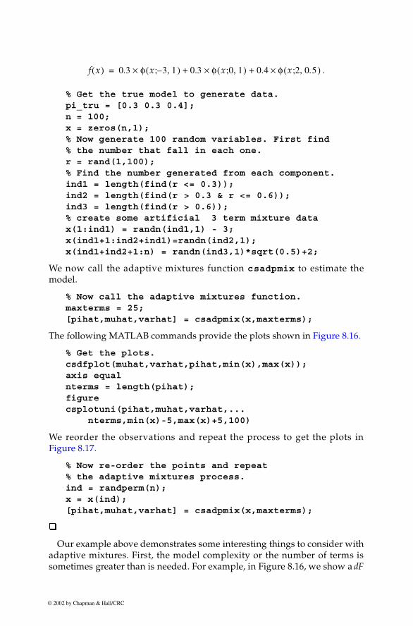
Chapter 8: Probability Density Estimation 305
.
% Get the true model to generate data.pi_tru = [0.3 0.3 0.4];n = 100;x = zeros(n,1);% Now generate 100 random variables. First find% the number that fall in each one.r = rand(1,100);% Find the number generated from each component.ind1 = length(find(r <= 0.3));ind2 = length(find(r > 0.3 & r <= 0.6));ind3 = length(find(r > 0.6));% create some artificial 3 term mixture datax(1:ind1) = randn(ind1,1) - 3; x(ind1+1:ind2+ind1)=randn(ind2,1); x(ind1+ind2+1:n) = randn(ind3,1)*sqrt(0.5)+2;
We now call the adaptive mixtures function csadpmix to estimate themodel.
% Now call the adaptive mixtures function.maxterms = 25;[pihat,muhat,varhat] = csadpmix(x,maxterms);
The following MATLAB commands provide the plots shown in Figure 8.16.
% Get the plots.csdfplot(muhat,varhat,pihat,min(x),max(x));axis equalnterms = length(pihat);figurecsplotuni(pihat,muhat,varhat,... nterms,min(x)-5,max(x)+5,100)
We reorder the observations and repeat the process to get the plots inFigure 8.17.
% Now re-order the points and repeat % the adaptive mixtures process.ind = randperm(n);x = x(ind);[pihat,muhat,varhat] = csadpmix(x,maxterms);
�
Our example above demonstrates some interesting things to consider withadaptive mixtures. First, the model complexity or the number of terms issometimes greater than is needed. For example, in Figure 8.16, we show a dF
f x( ) 0.3 φ x 3 1,–;( ) 0.3 φ x 0 1,;( )× 0.4 φ x 2 0.5,;( )×+ +×=
© 2002 by Chapman & Hall/CRC
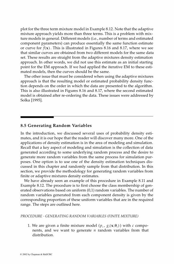
306 Computational Statistics Handbook with MATLAB
plot for the three term mixture model in Example 8.12. Note that the adaptivemixture approach yields more than three terms. This is a problem with mix-ture models in general. Different models (i.e., number of terms and estimatedcomponent parameters) can produce essentially the same function estimateor curve for . This is illustrated in Figures 8.16 and 8.17, where we seethat similar curves are obtained from two different models for the same dataset. These results are straight from the adaptive mixtures density estimationapproach. In other words, we did not use this estimate as an initial startingpoint for the EM approach. If we had applied the iterative EM to these esti-mated models, then the curves should be the same.
The other issue that must be considered when using the adaptive mixturesapproach is that the resulting model or estimated probability density func-tion depends on the order in which the data are presented to the algorithm.This is also illustrated in Figures 8.16 and 8.17, where the second estimatedmodel is obtained after re-ordering the data. These issues were addressed bySolka [1995].
8.5 Generating Random Variables
In the introduction, we discussed several uses of probability density esti-mates, and it is our hope that the reader will discover many more. One of theapplications of density estimation is in the area of modeling and simulation.Recall that a key aspect of modeling and simulation is the collection of datagenerated according to some underlying random process and the desire togenerate more random variables from the same process for simulation pur-poses. One option is to use one of the density estimation techniques dis-cussed in this chapter and randomly sample from that distribution. In thissection, we provide the methodology for generating random variables fromfinite or adaptive mixtures density estimates.
We have already seen an example of this procedure in Example 8.11 andExample 8.12. The procedure is to first choose the class membership of gen-erated observations based on uniform (0,1) random variables. The number ofrandom variables generated from each component density is given by thecorresponding proportion of these uniform variables that are in the requiredrange. The steps are outlined here.
PROCEDURE - GENERATING RANDOM VARIABLES (FINITE MIXTURE)
1. We are given a finite mixture model ( , ) with c compo-nents, and we want to generate n random variables from thatdistribution.
f x( )
pi gi x;θi( )
© 2002 by Chapman & Hall/CRC
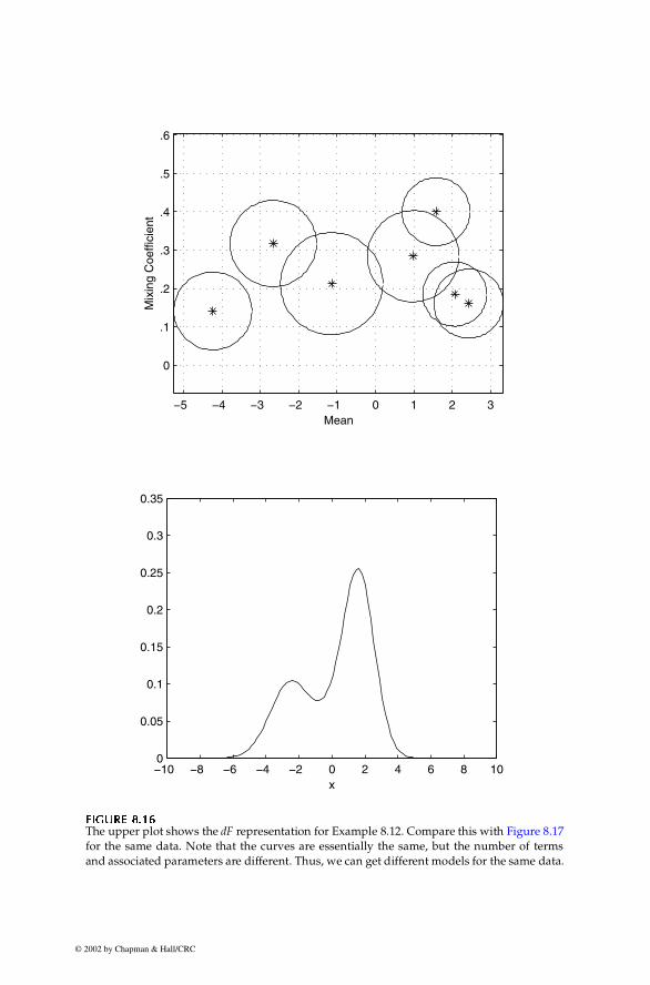
Chapter 8: Probability Density Estimation 307
FFFFIIIIGUGUGUGURE 8.1RE 8.1RE 8.1RE 8.16666
The upper plot shows the dF representation for Example 8.12. Compare this with Figure 8.17for the same data. Note that the curves are essentially the same, but the number of termsand associated parameters are different. Thus, we can get different models for the same data.
−5 −4 −3 −2 −1 0 1 2 3
0
.1
.2
.3
.4
.5
.6
Mean
Mix
ing
Coe
ffici
ent
−10 −8 −6 −4 −2 0 2 4 6 8 100
0.05
0.1
0.15
0.2
0.25
0.3
0.35
x
© 2002 by Chapman & Hall/CRC
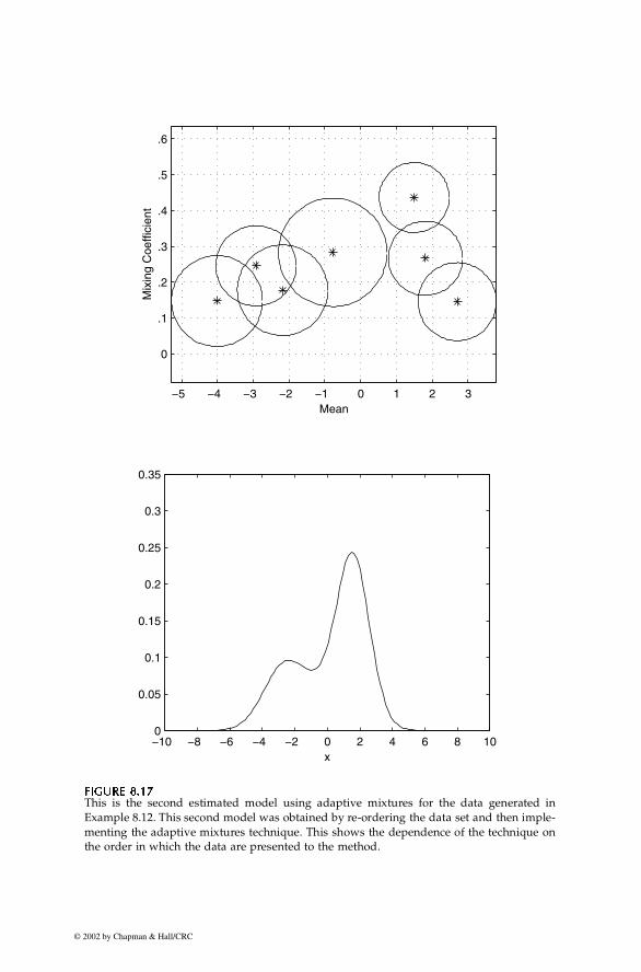
308 Computational Statistics Handbook with MATLAB
FFFFIIIIGUGUGUGURE 8.1RE 8.1RE 8.1RE 8.17777
This is the second estimated model using adaptive mixtures for the data generated inExample 8.12. This second model was obtained by re-ordering the data set and then imple-menting the adaptive mixtures technique. This shows the dependence of the technique onthe order in which the data are presented to the method.
−5 −4 −3 −2 −1 0 1 2 3
0
.1
.2
.3
.4
.5
.6
Mean
Mix
ing
Coe
ffici
ent
−10 −8 −6 −4 −2 0 2 4 6 8 100
0.05
0.1
0.15
0.2
0.25
0.3
0.35
x
© 2002 by Chapman & Hall/CRC
Chapter 8: Probability Density Estimation 309
2. First determine the component membership of each of the n randomvariables. We do this by generating n uniform (0,1) random vari-ables ( ). Component membership is determined as follows
If , then is from component density 1.
If , then is from component density 2.
. . .
If , then is from component density c.
3. Generate the from the corresponding using the compo-nent membership found in step 2.
Note that with this procedure, one could generate random variables from amixture of any component densities. For instance, the model could be a mix-ture of exponentials, betas, etc.
Example 8.13 Generate a random sample of size n from a finite mixture estimate of the OldFaithful Geyser data (geyser). First we have to load up the data and build afinite mixture model.
load geyser% Expects rows to be observations.data = geyser';% Get the finite mixture.% Use a two term model.% Set initial model to means at 50 and 80.muin = [50, 80];% Set mixing coefficients equal.piesin = [0.5, 0.5];% Set initial variances to 1.varin = [1, 1];max_it = 100;tol = 0.001;% Call the finite mixtures.[pies,mus,vars]=... csfinmix(data,muin,varin,piesin,max_it,tol);
Now generate some random variables according to this estimated model.
% Now generate some random variables from this model.% Get the true model to generate data from this.n = 300;x = zeros(n,1);
Ui
0 U≤ i p1< Xi
p1 U≤ i p1 p2+< Xi
pj U≤ i
j 1=
c 1–
∑ 1≤ Xi
Xi gi x;θ i( )
© 2002 by Chapman & Hall/CRC
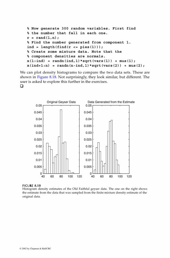
310 Computational Statistics Handbook with MATLAB
% Now generate 300 random variables. First find% the number that fall in each one.r = rand(1,n);% Find the number generated from component 1.ind = length(find(r <= pies(1)));% Create some mixture data. Note that the % component densities are normals.x(1:ind) = randn(ind,1)*sqrt(vars(1)) + mus(1); x(ind+1:n) = randn(n-ind,1)*sqrt(vars(2)) + mus(2);
We can plot density histograms to compare the two data sets. These areshown in Figure 8.18. Not surprisingly, they look similar, but different. Theuser is asked to explore this further in the exercises.�
FFFFIIIIGUGUGUGURE 8.1RE 8.1RE 8.1RE 8.18888
Histogram density estimates of the Old Faithful geyser data. The one on the right showsthe estimate from the data that was sampled from the finite mixture density estimate of theoriginal data.
40 60 80 100 1200
0.005
0.01
0.015
0.02
0.025
0.03
0.035
0.04
0.045
0.05Original Geyser Data
40 60 80 100 1200
0.005
0.01
0.015
0.02
0.025
0.03
0.035
0.04
0.045
0.05Data Generated from the Estimate
© 2002 by Chapman & Hall/CRC
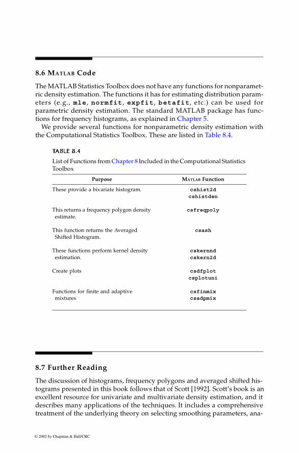
Chapter 8: Probability Density Estimation 311
8.6 MATLAB Code
The MATLAB Statistics Toolbox does not have any functions for nonparamet-ric density estimation. The functions it has for estimating distribution param-eters (e.g., mle , normfit , expfit , betafit, etc.) can be used forparametric density estimation. The standard MATLAB package has func-tions for frequency histograms, as explained in Chapter 5.
We provide several functions for nonparametric density estimation withthe Computational Statistics Toolbox. These are listed in Table 8.4.
8.7 Further Reading
The discussion of histograms, frequency polygons and averaged shifted his-tograms presented in this book follows that of Scott [1992]. Scott’s book is anexcellent resource for univariate and multivariate density estimation, and itdescribes many applications of the techniques. It includes a comprehensivetreatment of the underlying theory on selecting smoothing parameters, ana-
TTTTAAAABBBBLLLLEEEE 8.48.48.48.4
List of Functions from Chapter 8 Included in the Computational Statistics Toolbox
Purpose MATLAB Function
These provide a bivariate histogram. cshist2dcshistden
This returns a frequency polygon density estimate.
csfreqpoly
This function returns the Averaged Shifted Histogram.
csash
These functions perform kernel density estimation.
cskernndcskern2d
Create plots csdfplotcsplotuni
Functions for finite and adaptive mixtures
csfinmixcsadpmix
© 2002 by Chapman & Hall/CRC
312 Computational Statistics Handbook with MATLAB
lyzing the performance of density estimates in terms of the asymptotic meanintegrated squared error, and also addresses high dimensional data.
The summary book by Silverman [1986] provides a relatively non-theoret-ical treatment of density estimation. He includes a discussion of histograms,kernel methods and others. This book is readily accessible to most statisti-cians, data analysts or engineers. It contains applications and computationaldetails, making the subject easier to understand.
Other books on density estimation include Tapia and Thompson [1978],Devroye and Gyorfi [1985], Wand and Jones [1995], and Simonoff [1996]. TheTapia and Thompson book offers a theoretical foundation for density estima-tion and includes a discussion of Monte Carlo simulations. The Devroye andGyorfi text describes the underlying theory of density estimation using the
(absolute error) viewpoint instead of (squared error). The books byWand and Jones and Simonoff look at using kernel methods for smoothingand exploratory data analysis.
A paper by Izenman [1991] provides a comprehensive review of manymethods in univariate and multivariate density estimation and includes anextensive bibliography. Besides histograms and kernel methods, he discussesprojection pursuit density estimation [Friedman, Stuetzle, and Schroeder,1984], maximum penalized likelihood estimators, sieve estimators, andorthogonal estimators.
For the reader who would like more information on finite mixtures, we rec-ommend Everitt and Hand [1981] for a general discussion of this topic. Thebook provides a summary of the techniques for obtaining mixture models(estimating the parameters) and illustrates them using applications. That textalso discusses ways to handle the problem of determining the number ofterms in the mixture and other methods for estimating the parameters. It isappropriate for someone with a general statistics or engineering background.For readers who would like more information on the theoretical details offinite mixtures, we refer them to McLachlan and Basford [1988] or Tittering-ton, Smith and Makov [1985]. A recent book by McLachlan and Peel [2000]provides many examples of finite mixtures, linking them to machine learn-ing, data mining, and pattern recognition.
The EM algorithm is described in the text by McLachlan and Krishnan[1997]. This offers a unified treatment of the subject, and provides numerousapplications of the EM algorithm to regression, factor analysis, medical imag-ing, experimental design, finite mixtures, and others.
For a theoretical discussion of the adaptive mixtures approach, the readeris referred to Priebe [1993, 1994]. These examine the error in the adaptive mix-tures density estimates and its convergence properties. A recent paper byPriebe and Marchette [2000] describes a data-driven method for obtainingparsimonious mixture model estimates. This methodology addresses someof the problems with the adaptive/finite mixtures approach: 1) that adaptivemixtures is not designed to yield a parsimonious model and 2) how manyterms or component densities should be used in a finite mixture model.
L1 L2
© 2002 by Chapman & Hall/CRC
Chapter 8: Probability Density Estimation 313
Solka, Poston, and Wegman [1995] extend the static dF plot to a dynamicone. References to MATLAB code are provided in this paper describing adynamic view of the adaptive mixtures and finite mixtures estimation pro-cess in time (i.e., iterations of the EM algorithm).
© 2002 by Chapman & Hall/CRC
314 Computational Statistics Handbook with MATLAB
Exercises
8.1. Create a MATLAB function that will return the value of the histogram estimate for the probability density function. Do this for the 1-D case.
8.2. Generate a random sample of data from a standard normal. Construct a kernel density estimate of the probability density function and verifythat the area under the curve is approximately 1 using trapz.
8.3. Generate 100 univariate normals and construct a histogram. Calculate the MSE at a point using Monte Carlo simulation. Do this forvarying bin widths. What is the better bin width? Does the samplesize make a difference? Does it matter whether is in the tails orcloser to the mean? Repeat this experiment using the absolute error.Are your conclusions similar?
8.4. Generate univariate normal random variables. Using the Normal Ref-erence Rules for h, construct a histogram, a frequency polygon and akernel estimate of the data. Estimate the MSE at a point usingMonte Carlo simulation.
8.5. Generate a random sample from the exponential distribution. Con-struct a histogram using the Normal Reference Rule. Using MonteCarlo simulation, estimate the MISE. Use the skewness factor to adjusth and re-estimate the MISE. Which window width is better?
8.6. Use the snowfall data and create a MATLAB movie that showshow 1-D histograms change with bin width. See help on movie forinformation on how to do this. Also make a movie showing howchanging the bin origin affects the histogram.
8.7. Repeat Example 8.2 for bin widths given by the Freedman-Diaconis Rule. Is there a difference in the results? What does the histogramlook like if you use Sturge’s Rule?
8.8. Write a MATLAB function that will return the value of a bivariatehistogram at a point, given the bin counts, the sample size, and thewindow widths.
8.9. Write a MATLAB function that will evaluate the cumulative distribu-tion function for a univariate frequency polygon. You can use thetrapz, quad, or quadl functions.
8.10. Load the iris data. Create a matrix by concatenating thefirst two columns of each species. Construct and plot a frequencypolygon of these data. Do the same thing for all possible pairs ofcolumns. You might also look at a contour plot of the frequencypolygons. Is there evidence of groups in the plots?
x0
x0
x0
150 2×
© 2002 by Chapman & Hall/CRC
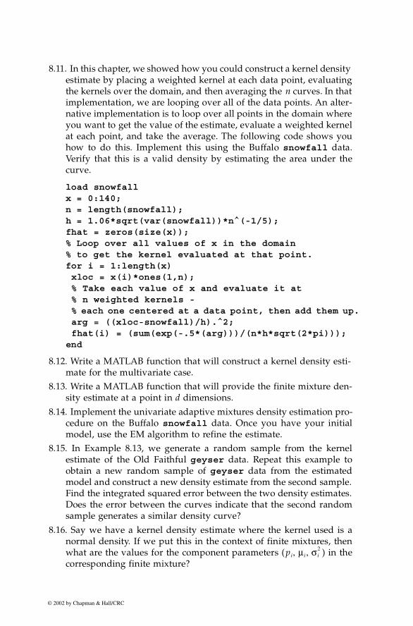
Chapter 8: Probability Density Estimation 315
8.11. In this chapter, we showed how you could construct a kernel density estimate by placing a weighted kernel at each data point, evaluatingthe kernels over the domain, and then averaging the n curves. In thatimplementation, we are looping over all of the data points. An alter-native implementation is to loop over all points in the domain whereyou want to get the value of the estimate, evaluate a weighted kernelat each point, and take the average. The following code shows youhow to do this. Implement this using the Buffalo snowfall data.Verify that this is a valid density by estimating the area under thecurve.
load snowfallx = 0:140;n = length(snowfall);h = 1.06*sqrt(var(snowfall))*n^(-1/5);fhat = zeros(size(x));% Loop over all values of x in the domain% to get the kernel evaluated at that point.for i = 1:length(x)xloc = x(i)*ones(1,n);% Take each value of x and evaluate it at % n weighted kernels - % each one centered at a data point, then add them up. arg = ((xloc-snowfall)/h).^2;fhat(i) = (sum(exp(-.5*(arg)))/(n*h*sqrt(2*pi)));
end
8.12. Write a MATLAB function that will construct a kernel density esti-mate for the multivariate case.
8.13. Write a MATLAB function that will provide the finite mixture den-sity estimate at a point in d dimensions.
8.14. Implement the univariate adaptive mixtures density estimation pro-cedure on the Buffalo snowfall data. Once you have your initialmodel, use the EM algorithm to refine the estimate.
8.15. In Example 8.13, we generate a random sample from the kernelestimate of the Old Faithful geyser data. Repeat this example toobtain a new random sample of geyser data from the estimatedmodel and construct a new density estimate from the second sample.Find the integrated squared error between the two density estimates.Does the error between the curves indicate that the second randomsample generates a similar density curve?
8.16. Say we have a kernel density estimate where the kernel used is anormal density. If we put this in the context of finite mixtures, thenwhat are the values for the component parameters ( ) in thecorresponding finite mixture?
pi, µi, σ i2
© 2002 by Chapman & Hall/CRC
316 Computational Statistics Handbook with MATLAB
8.17. Repeat Example 8.12. Plot the curves from the estimated models.What is the ISE between the two estimates? Use the iterative EMalgorithm on both models to refine the estimates. What is the ISE afteryou do this? What can you say about the two different models? Areyour conclusions different if you use the IAE?
8.18. Write a MATLAB function that will generate random variables(univariate or multivariate) from a finite mixture of normals.
8.19. Using the method for generating random variables from a finitemixture that was discussed in this chapter, develop and implementan algorithm for generating random variables based on a kernel den-sity estimate.
8.20. Write a function that will estimate the MISE between two functions.Convert it to also estimate the MIAE between two functions.
8.21. Apply some of the univariate density estimation techniques fromthis chapter to the forearm data.
8.22. The elderly data set contains the height measurements (in centi-meters) of 351 elderly females [Hand, et al., 1994]. Use some of theunivariate density estimation techniques from this chapter to explorethe data. Is there evidence of bumps and modes?
8.23. Apply the multivariate techniques of this chapter to the nfl data[Csorgo and Welsh, 1989; Hand, et al., 1994]. These data contain bivari-ate measurements of the game time to the first points scored bykicking the ball between the end posts ( ), and the game time tothe first points scored by moving the ball into the end zone ( ).The times are in minutes and seconds. Plot your results.
X1
X2
© 2002 by Chapman & Hall/CRC