Chapter 8 Origin of Turbulence and Turbulent Shear Stress
57
Ch 8. Origin of Turbulence and Turbulent Shear Stress 8-1 Chapter 8 Origin of Turbulence and Turbulent Shear Stress 8.1 Introduction 8.1.1 Definition • Hinze (1975): Turbulent fluid motion is an irregular condition of flow in which the various quantities show a random variation with time and space coordinates, so that statistically distinct average values can be discerned. statistically distinct average values: mean flow, primary motion random fluctuations: non-periodic, secondary motion, instantaneously unsteady, varies w.r.t. time and space • Types of turbulence wall turbulence … turbulence generated and continuously affected by actual physical boundary such as solid walls free turbulence … absence of direct effect of walls, turbulent jet 8.1.2 Origin of turbulence (1) Shear flow instability
Transcript of Chapter 8 Origin of Turbulence and Turbulent Shear Stress

Ch 8. Origin of Turbulence and Turbulent Shear Stress
8-1
Chapter 8 Origin of Turbulence and Turbulent Shear Stress
8.1 Introduction
8.1.1 Definition
• Hinze (1975): Turbulent fluid motion is an irregular condition of flow in which the
various quantities show a random variation with time and space coordinates, so that
statistically distinct average values can be discerned.
statistically distinct average values: mean flow, primary motion
random fluctuations: non-periodic, secondary motion,
instantaneously unsteady, varies w.r.t. time and space
• Types of turbulence
wall turbulence … turbulence generated and continuously affected by actual physical
boundary such as solid walls
free turbulence … absence of direct effect of walls, turbulent jet
8.1.2 Origin of turbulence
(1) Shear flow instability

Ch 8. Origin of Turbulence and Turbulent Shear Stress
8-2
(2) Boundary-wall-generated turbulence
~ wall turbulence
(3) Free-shear-layer-generated turbulence
~ free turbulence
1) jet
2) wakes
3) mixing layer
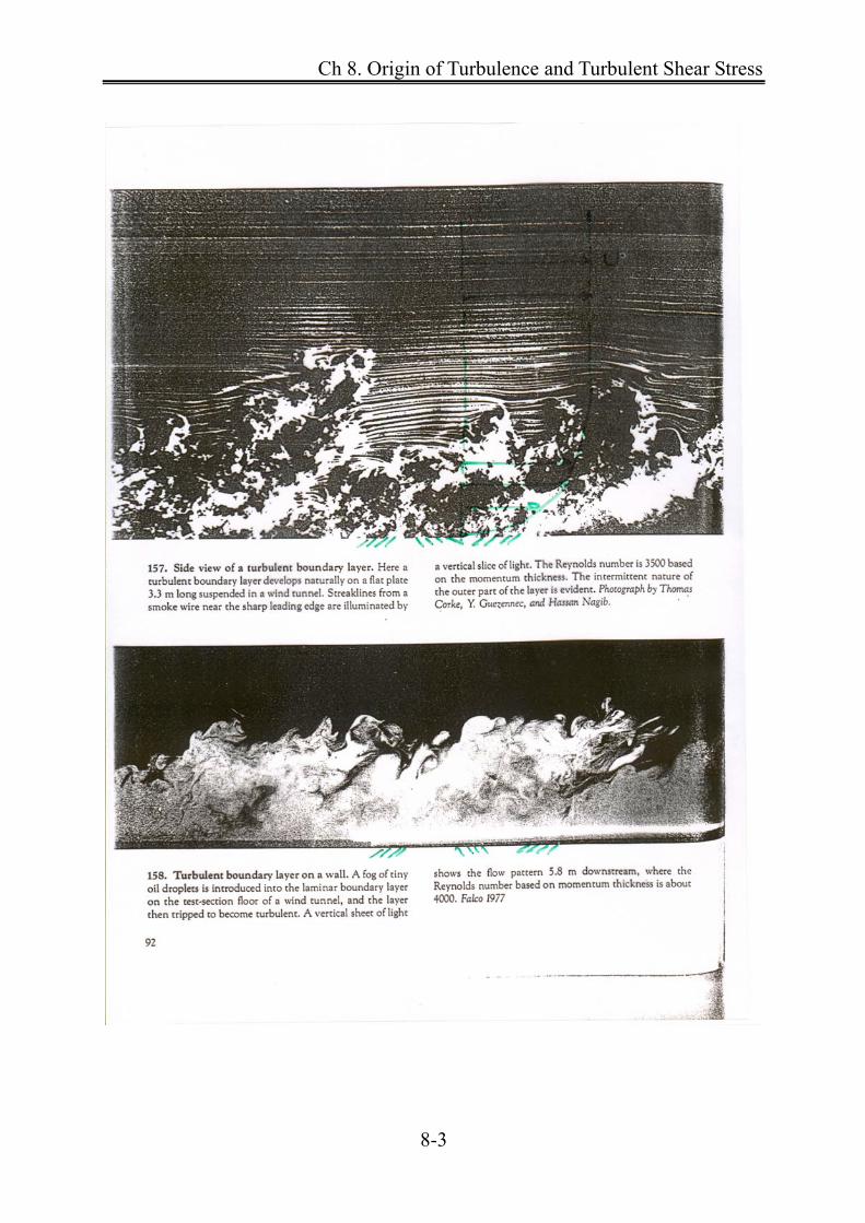
Ch 8. Origin of Turbulence and Turbulent Shear Stress
8-3

Ch 8. Origin of Turbulence and Turbulent Shear Stress
8-4

Ch 8. Origin of Turbulence and Turbulent Shear Stress
8-5

Ch 8. Origin of Turbulence and Turbulent Shear Stress
8-6

Ch 8. Origin of Turbulence and Turbulent Shear Stress
8-7
8.1.3 Nature of turbulence
(1) Irregularity
∼ randomness
∼ need to use statistical methods to turbulence problems
∼ Turbulent motion can also be described by Navier-Stokes Eq.
[Cf] Coherent structure
(2) Diffusivity
∼ causes rapid mixing and increased rates of momentum, heat, and mass transfer
∼ exhibit spreading of velocity fluctuations through surrounding fluid
∼ the most important feature as far as practical applications are concerned; it increases
heat transfer rates in machinery, it increases mass transfer in water
(3) Large Reynolds numbers
∼ occur at high Reynolds numbers
∼ Turbulence originates as an instability of laminar flows if Re becomes too large.
pipe flow Re 2,000c
boundary layer Re 600c
U
free shear flow Re ~c low
(4) Three-dimensional vorticity fluctuations
∼ Turbulence is rotational and three-dimensional.

Ch 8. Origin of Turbulence and Turbulent Shear Stress
8-8
∼ high levels of fluctuating vorticity
∼ need to use vorticity dynamics
∼tend to be isotropic
[Cf] The 2-D flows like cyclones, random (irrotational) waves in the ocean are not turbulent
motions.
(5) Dissipations
∼ dissipative
∼ deformation work increases the internal energy of the fluid while dissipating kinetic
energy of the turbulence
∼ needs a continuous supply of energy to make up for viscous losses.
∼ main energy supply comes from mean flow by interaction of shear stress and velocity
gradient
∼ If no energy is supplied, turbulence decays rapidly.
[Re] Energy cascade
Main flow → large scale turbulence → small scale turbulence→ heat
(6) Continuum
∼ continuum phenomenon
∼ governed by the equation of fluid mechanics: Navier-Stokes Eq. + Continuity Eq.
∼ larger than any molecular length scale

Ch 8. Origin of Turbulence and Turbulent Shear Stress
8-9
(7) Flow
∼ feature of fluid flows not fluid itself
∼ Most of the dynamics of turbulence is the same in all fluids.
∼ Major characteristics of turbulent flows are not controlled by the molecular properties of
the fluid.
8.1.4 Description of turbulence problems
(1) Turbulence modeling
• Time-averaged Navier-Stokes Eq. → Reynolds Equations
→ No. of unknowns {mean values( , , ,u v w p ) + Reynolds stress components
( ', ' )ij i ju u } > No. of equations
→ Closure problem:
∼ The gap (deficiency of equations) can be closed only with models and estimates based on
intuition and experience.
(2) Methods of analysis
1) Phynomenological concepts of turbulence
∼ based on a superficial resemblance between molecular motion and turbulent motion
∼ crucial assumptions at a early stage in the analysis
• Eddy viscosity model
∼ turbulence-generated viscosity is modeled using analogy with molecular viscosity
∼ characteristics of flow

Ch 8. Origin of Turbulence and Turbulent Shear Stress
8-10
• Mixing length model
∼ analogy with mean free path of molecules in the kinetic theory of gases
2) Dimensional analysis
∼ one of the most powerful tools
∼ result in the relation between the dependent and independent variables
[Ex] form of the spectrum of turbulent kinetic energy
3) Asymptotic theory
∼ based on asymptotic invariance
∼ exploit asymptotic properties of turbulent flows as Re approaches infinity (or very
high).
[Ex)] Theory of turbulent boundary layers
Reynolds-number similarity
4) Deterministic approach
∼ large eddy simulation (L.E.S)
5) Stochastic approach

Ch 8. Origin of Turbulence and Turbulent Shear Stress
8-11
8.2 Sources of Turbulence
8.2.1 Source of turbulence
(1) Surfaces of flow discontinuity (velocity discontinuity)
1) tip of sharp projections
2) the trailing edges of air foils and guide vanes
3) zones of boundary-layer separation
At surfaces of flow discontinuity,
→ tendency for waviness to develop by accident from external cause or from disturbance
transported by the fluid.
→ waviness tends to be unstable
→ amplify (grow in amplitude)
→ curl over
→ break into separate eddies

Ch 8. Origin of Turbulence and Turbulent Shear Stress
8-12
(2) Shear flows where velocity gradient occurs w/o an abrupt discontinuity
~ Shear flow is becoming unstable and degenerating into turbulence.
[Ex] Reynolds' experiment with a dye-streak in a glass tube
[Re] How turbulence arises in a flow
1) Presence of boundaries as obstacles creates vorticity inside a flow which was initially
irrotational. (vorticity, u
)
2) Vorticity produced in the proximity of the boundary will diffuse throughout the flow which
will become turbulent in the rotational regions.
3) Production of vorticity will then be increased due to vortex filaments stretching mechanism.
[Re] Grid turbulence = turbulence created behind a fixed grid in a wind tunnel
convex side - low pressure
(high velocity)
concave side - high pressure
(low velocity)

Ch 8. Origin of Turbulence and Turbulent Shear Stress
8-13
8.2.2 Mechanisms of instability
• Tollmien-Schlichting's small perturbation theory
∼ Disturbance are composed of oscillations of a range of frequencies which can be
selectively amplified by the hydrodynamic flow field.
Re < Recrit , all disturbances will be damped
Re > Recrit , disturbances of certain frequencies will be amplified and others damped
• Tollmien-Schlichting stability diagram

Ch 8. Origin of Turbulence and Turbulent Shear Stress
8-14
• Disturbances appear in spots
∼ These spots grow as they are swept downstream.
∼ spread and amplification of a spot disturbance into a turbulence patch
∼ Mechanism of the initiation of spots of turbulence is related to what happens when the
small disturbance, whose amplification is predicted by the small-perturbation theory, become
large.

Ch 8. Origin of Turbulence and Turbulent Shear Stress
8-15
Pipe flow: 10-1~100 sec
River flow: 100~101 sec
8.3 Velocities, Energies, and Continuity in Turbulence
8.3.1 Reynolds decomposition
(1) Velocity decomposition
'u u u
'v v v
'w w w (8.1)
, ,u v w = instantaneous velocity
, ,u v w = mean value = time-averaged value
' , ' , 'u v w = fluctuating components
0
1 Tu u dt
T (steady flow; 0
u
t
) (8.2)
where T = long time compared to the time scale of the turbulence
0
1' ' 0
Tu u dt
T (∵ fluctuations are both plus and minus) (8.3)
0
1( ) 0
Tu u d t u u
T
(2) Pressure and stress decomposition
'p p p

Ch 8. Origin of Turbulence and Turbulent Shear Stress
8-16
' 0p
'ij ij ij
' 0ij
• Mean stress tensor
2ij ij ijp S
' ' 2 'ij ij ijp S
in which ijS = mean strain rate1
2ji
j i
uu
x x
'ijS = strain-rate fluctuations''1
2ji
j i
uu
x x
(3) Intensity of turbulence
→ root-mean-square (rms) = square root of variance = standard deviation average intensity
of the turbulence = rms of u'
=
1
22 2
0
1' '
Tu u dt
T (8.4)
• Relative intensity of turbulence =2'u
u

Ch 8. Origin of Turbulence and Turbulent Shear Stress
8-17
(4) Average kinetic energy of turbulence per unit mass
∼ average KE of turbulence / mass
2 2 2
2
1( ' ' ' )
2
1( )
2
u v w
intensity
(8.5)
(5) Energy density, ( )f
The kinetic energy is decomposed into an energy spectrum (density) vs frequency.
≡ limit of average kinetic energy per unit mass divided by the bandwidth f
0
/( ) lim
f
averageKE mass contained in f Kf
f f
where f = ordinary frequency in cycles per second = 2
∴ average KE of turbulence / mass
= 2 2 2
0
1( ) ( ' ' ' )
2f df u v w
(6) Correlation between u', v', and w'
exact correlation = one-to-one correlation
zero correlation = completely independent

Ch 8. Origin of Turbulence and Turbulent Shear Stress
8-18
0
01' ' ' '
0
T correlatedu v u v dt
uncorrelatedT
(8.6)
~ In a shear flow in an xy-plane, ' 'u v is finite, and it is related to the magnitude of the
turbulent shear stress ( ' 'u v ).
[Re] Correlated variables
1) Averages of products u
( ')( ')
' ' '
i j i i j j
i j i j i j
u u u u u u
u u u u u u
'j iu u
' 'i j i ju u u u
If ' ' 0 'i j iu u u and 'ju are said to be correlated.
If ' ' 0 'i j iu u u and 'ju are uncorrelated.
2) Correlation coefficient
1/22 2
' '
( ' ' )
u ui j
cij
u ui j
in which 2 2' , 'i ju u = variances
If 1ijc → perfect correlation

Ch 8. Origin of Turbulence and Turbulent Shear Stress
8-19
[Re] Classification of turbulence
1) General turbulence
u v w
2 2 2' ' 'u v w
' ' ' ' ' 'u v v w w u
2) Homogeneous turbulence
~ statistically independent of the location
( ' ') ( ' ')i j a i j bu u u u
3) Isotropic turbulence
~ statistically independent of the orientation and location of the coordinate axes
2 2 2' ' 'u v w = constant
' ' ' ' ' ' 0u v v w w u
∼ uncorrelated
∼ not coherent structures
8.3.2 Measurement of turbulence
∼ measure turbulent fluctuations
(1) Hot-wire (hot-film) anemometer
∼ Hot-film is usable in contaminated water.

Ch 8. Origin of Turbulence and Turbulent Shear Stress
8-20
~ Change of temperature affects the electric current flow or voltage drop through wire. Fine
platinum wire (film) is heated electrically by a circuit that maintains voltage drop constant.
~ When inserted into the stream, the cooling, which is a function of the velocity, can be
detected as variations in voltage.
~ Use two or more wires at one point in the flow to make simultaneous measurements of
different velocity components.
→ After subtracting mean value, rms-values, correlations, and energy spectra can be
computed using fluctuation.
→ These operations can be performed electronically
(2) Laser Doppler Velocimeter (LDV)
~ Doppler effects
~ An laser (ultrasonic) beam transmitted into the fluid will be reflected by impurities or
bubbles in the fluid to a receiving sensor at a different frequency.
→ The transmitted and reflected signals are then compared by electronic means to calculate
the Doppler shift which is proportional to the velocity.
~ non-intrusive sensing (immersible LDA)
~ sampling frequency = 20,000 Hz

Ch 8. Origin of Turbulence and Turbulent Shear Stress
8-21
(3) Acoustic Doppler Velocimeter (ADV)
~ use Doppler effects
~ intrusive sensing
~ sampling frequency = 25-50 Hz
(4) Particle Image Velocimetry (PIV)
~ use Laser and CCD camera
~ measure flow field at once
~ sampling frequency = 30 Hz

Ch 8. Origin of Turbulence and Turbulent Shear Stress
8-22
PIV system
Velocity of particle A: 0x
xu as t
t
0y
yu as t
t

Ch 8. Origin of Turbulence and Turbulent Shear Stress
8-23
LDV: single point measurement
PIV: field measurement
a) Image b)Velocity c)Turbulence Intensity
Fig. 1 Jet Characteristics Measured by PIV (Seo et al., 2002)

Ch 8. Origin of Turbulence and Turbulent Shear Stress
8-24
[Re] Reynolds rules of averages: Schlichting (1979) Boundary-Layer Theory
Let f and g are two dependent variables whose time mean values are to be found. s is any
one of the independent variables x, y, z, t.
f f
f g f g
f g f g
since time averaging is carried out by integrating over a long
period of time,which commutes with differentiation with respect
to another independant variable
f f
s s
f ds f ds
8.3.3 Continuity for turbulent motion
Continuity equation for incompressible fluid
0u v w
x y z
(A)
Substitute velocity decomposition into (A)
( ') ( ') ( ')0
u u v v w w
x y z
(8.7)
' ' '0
u v w u v w
x y z x y z
(B)

Ch 8. Origin of Turbulence and Turbulent Shear Stress
8-25
Take time-averages of each term of (B)
'u v w u
x y z x
'v
y
'w
z
0
' ( ')0
u u
x x
0u v w
x y z
(8.8)
Substitute (8.8) into (B)
' ' '0
u v w
x y z
(8.9)
→ Both mean-motion components and the superposed turbulent-motion components must
satisfy the continuity equation.
→ Continuity must be satisfied for both turbulent and laminar motions.
[Re] Continuity Eq. for compressible fluid
0i
i
u
t x
( ')( ')( ')0
i i
i
u u
t x

Ch 8. Origin of Turbulence and Turbulent Shear Stress
8-26
Time averaging yields
{( ')( ')}( ')0i i
i
u u
t x
'
t t
( 'i i
i
u ux
'iu ' ') 0iu
( ' ') 0i ii
u ut x
( ' ') ( ' ') ( ' ') 0u v w
u v wt x y z x y z

Ch 8. Origin of Turbulence and Turbulent Shear Stress
8-27
8.4 Turbulent Shear Stress and Eddy Viscosities
8.4.1 Fall of pressure drop due to shear stress
shear stress = resistance to motion
→ dissipate flow energy → fall of pressure drop along a pipe → head loss ('
L
lh
R
)
Laminar flow; ( )
z
d p hV
dz
∝
Turbulent flow: ( )
∝ nz
d p hV
dz
( 2n )
where zV = average velocity
8.4.2 Shear stress resisting to motion
(1) Boussinesq's eddy viscosity concept
total
du du
dy dy (8.10)
Laminar flow
Turbuent flow

Ch 8. Origin of Turbulence and Turbulent Shear Stress
8-28
where
u = mean local velocity (time - averaged)
μ = dynamic molecular viscosity → property of the fluid
= dynamic eddy viscosity that depends on the state of the turbulent motion
(
= kinematic eddy viscosity)
du
dy - apparent stress computed from the velocity gradient of mean motion.
du
dy - additional apparent stress associated with the turbulence
For laminar flow, 0
For turbulent flow, → turb lam
(2) Physical model of momentum transport (exchange)
∼ momentum transport by turbulent velocity fluctuation

Ch 8. Origin of Turbulence and Turbulent Shear Stress
8-29
Step 1: lower-velocity fluid parcel in layer 1 fluctuates with a v'-velocity into
layer 2
Step 2: its velocity in the direction of the stream is less than mean velocity of the
layer 2 by an amount -u'
Step 3: Drag of the faster moving surroundings accelerates the fluid element and
increases its momentum
Step 4: The mass flux crossing from layer 1 to layer 2
= 'mass
vtime area
Step 5: Flow-direction momentum change = mass × velocity
= ' ( ') ' 'v u u v
Step 6: Average over a time period
= ' 'u v
= effective resistance to motion
= effective shearing stress
(3) Reynolds stress
= ' 'u v (8.11)
= time rate change of momentum per unit area
= effective resistance to motion
~ actually acceleration terms
~ instantaneous viscous stresses due to turbulent motion = du
dy

Ch 8. Origin of Turbulence and Turbulent Shear Stress
8-30
' 'total yx
duu v
dy
(8.12)
shear stress shear stress due to
due to transverse transverse momentum transport of
molecular momentum macroscopic fluid particles by
transport turbulent motion
For fully developed turbulence,
2' 'yx z
duu v V
dy
(8.13)
[Re] Reynolds stress = ' 'u v
~ If u' and v' are uncorrelated, there would be no turbulent momentum transport.
~ usually not zero (correlated)
~ may exchange momentum of mean motion
~ exchanges momentum between turbulence and mean flow
[Re] Effective addition to the normal pressure intensity acting in the flow direction
= 2' ' 'u u u (8.14)
[Re] Momentum transport
Eq. (3.2): ( ) 1d mv d mv
Kdt area dy vol

Ch 8. Origin of Turbulence and Turbulent Shear Stress
8-31
Newton's 2nd law of motion
( )dv d mvF ma m
dt dt (A)
( ) 1F d mv
area dt area (B)
Assume only shear stresses exist,
Then LHS of (B) = τ
Combine (3. 2) & (B)
du
dy (C)
By the way, for the turbulent motion
RHS of (B) = time rate change of momentum per unit area = ' 'u v
' 'u v (D)
Combine (C) and (D)
' 't
duu v
dy (E)

Ch 8. Origin of Turbulence and Turbulent Shear Stress
8-32
[Re] Shear stress for turbulent jet
Case I: 0du
dy → positive
1) 1 1y y
mass flux = 'v
velocity change = 'u
∴ momentum change = ( ') ( ') ' 'v u u v
' 'u v → + momentum change → positive
2) 1 1y y
mass flax = ( ')v
velocity change = 'u+
∴ momentum change = ( ') ( ') ' 'v u u v
' 'u v → + momentum change → positive

Ch 8. Origin of Turbulence and Turbulent Shear Stress
8-33
Case II: 0du
dy → negative
1) 1 1' 'y y
mass flax = 'v
velocity change = 'u
∴ momentum change = ( ') ( ') ' 'v u u v
' 'u v → - momentum change → negative
2) 1 1' 'y y
mass flux = ( ')v
velocity change = 'u
∴ momentum change = ( ') ( ') ' 'v u u v
' 'u v → - momentum change → negative

Ch 8. Origin of Turbulence and Turbulent Shear Stress
8-34

Ch 8. Origin of Turbulence and Turbulent Shear Stress
8-35
8.5 Reynolds Equations for Incompressible Fluids
8.5.1 Reynolds Equation
Navier-Stokes Eq. = equations of motion of a viscous fluid
~ applicable to both turbulent and non-turbulent flows
~ very difficult to obtain exact solution because of complexity of turbulence
~ Alternative is to consider the pattern of the mean turbulent motion even through we
cannot establish the true details of fluctuations.
→ average Navier-Stokes Eq. over time to derive Reynolds Eq.
N-S Eq. in x-dir.:
yxx zxx
pu u u uu v w g
t x y z x y z
(8.15)
Continuity Eq. for incompressible fluid:
0u v w
u u ux y z
(A)
Add (A) to (11.15)
LHS =2
2u u u v u w u u uv uw
u v u w ut x y y z z t x y z
Substituting this yields
2yxx zx
x
pu u uv uwg
t x y z x y z
(8.16)

Ch 8. Origin of Turbulence and Turbulent Shear Stress
8-36
Decomposition:
'u u u
'v v v
'w w w
'x x xp p p (8.17)
Substitute (8.17) into (8.16), and average over time
2( ') ( ') ( ')( ') ( ')( ')
( ') yxx x zxx
u u u u u u v v u u w w
t x y z
p pg
x y z
Rearrange according to the Reynolds average rule
( ') 'u u u u
t t t
u
t
2 2 22 2( ') '
( 2 ' ' )u u u u
u uu ux x x x
( ')( ')( '
u u v vu v uv
y y
'u v
' '' ')
u v u vu v
y y
( ')( ')( '
u u w wu w u w
z z
'u w
' '' ')
u w u wu w
z z
2
2' ' ' ' '
yxx zxx
u u u v u w pg
t x y z x y z
u u v u w
x y z

Ch 8. Origin of Turbulence and Turbulent Shear Stress
8-37
Subtract Continuity Eq. of mean motion ( 0u v w
u u ux y z
)
2
2' ' ' ' 'yxx zxx
u u u v u w u v wu u u
t x y z x y z
p u u v u wg
x y z x y z
2' ' ' ' 'yx zyxx
u u u uu v w
t x y z
p u u v u wg
x y z x y z
(8.18)
~
y-direction:
2' ' ' ' '
xy y zyy
pv v v vu v w g
t x y z x y z
v u v v w
x y z
z-direction:
2' ' ' ' '
yzxz zz
w w w w pu v w g
t x y z x y z
w u w v w
x y z
•turbulence acceleration terms
•mean transport of fluctuating momentum
by turbulent velocity fluctuations

Ch 8. Origin of Turbulence and Turbulent Shear Stress
8-38
Rearrange (8.18)
2' ( ' ') ( ' ')x x yx zx
u u u uu v w
t x y z
g p u u v u wx y z
Introduce Newtonian stress relations: Eqs. 5.29 & 5.30
22
3x
up q
x
22
3y
vp q
y
22
3z
wp q
z
yx xy
v u
x y
yz zy
w v
y z
zx xz
u w
z x
Substitute velocity decomposition, Eqs (8.17) into Eqs. (5.29) & (5.30) and average over time
for incompressible fluid ( 0q
)
Sum of apparent stress of the mean motion and additional apparent stress due to turbulent fluctuations

Ch 8. Origin of Turbulence and Turbulent Shear Stress
8-39
1) x-direction:
( )( ') 2 2x x
u u up p p p
x x
'
( ') ( ')yx
v v u u v u
x y x y
( ') ( ')zx
u u w w u w
z x z x
(8.20 a)
(2) y-direction:
2y
vp p
y
xy
v u
x y
zyw v
y z
(8.20 b)
(3) z-direction:
2z
wp p
z
xz
u w
z x
yz
w v
y z
(8.20 c)

Ch 8. Origin of Turbulence and Turbulent Shear Stress
8-40
Substitute Eq. (8.20) into Eq. (8.18)
2
2
' ' ' ' '
x
u u u uu v w
t x y z
u v u u wg p
x x y x y z z x
u u v u w
x y z
2 2 2 2 2
2 2 2
2
2
' ' ' ' '
x
p u v u u wg
x x y x y z z x
u u v u w
x y z
2 2 2 2 2 2
2 2 2 2
2
2
( )
' ' ' ' '
x
p u u u u v wg
x x y z x y x z x
u
u u v u w
x y z
By the way,
(I) = 0u v w
x x y z
(∵ Continuity Eq. for incompressible fluid)
Therefore, substituting this relation yields

Ch 8. Origin of Turbulence and Turbulent Shear Stress
8-41
x-dir.:
22 ' ' ' ' '
x
u u u uu v w
t x y z
p u u v u wg u
x x y z
(8.22 a)
y-dir.:
22 ' ' ' ' '
y
v v v vu v w
t x y z
p v u v v wg v
y x y z
(8.22 b)
z-dir.:
22 ' ' ' ' '
z
w w w wu v w
t x y z
p w u w v wg w
z x y z
(8.22 c)
→ Reynolds Equations (temporal mean eq. of motion)
→ Navier-Stokes form for incompressible fluid
[Re] No. of Equations = 4
No. of Unknowns: 4 + 9 (turbulence fluctuating terms)
→ 9 products of ' 'i ju u
→ one-point double correlation of velocity fluctuation

Ch 8. Origin of Turbulence and Turbulent Shear Stress
8-42
[Re]
1) Reynolds Equation of motion → solve for mean motion
21( ' ' )i i i
j i j ij j i j j
u u upu u u X
t x x x x x
time rate of body change of force momentum rate of convection
to mean of the force due momentum to mean
pressure rate of diffusion rate of molecular of momentum diffusion of by turbulence momentum
by viscosity
2) Navier-Stokes Eq. → apply to instantaneous motion
21i i ij i
j i j j
u u p uu X
t x x x x
8.5.2 Closure Model
Assumptions are needed to close the gap between No. of equations and No. unknowns.
→ Turbulence modeling: Ch. 10
■ Boussinesq's eddy viscosity model
2'
' '
' '
x
y
z
uu
x
uu v
y
uu w
z
(A)

Ch 8. Origin of Turbulence and Turbulent Shear Stress
8-43
Reynolds Equation in x-dir.:
2 2 2 2
2 2 2
' ' ' ' 'x
u u u uu v w
t x y z
p u u u u u v u wg
x x y z x y z
2' ' ' ' 'x
p u u ug u u v u w
x x x y y z z
(B)
Substitute (A) and into (B)
( ) ( ) ( )x x y z
u u u uu v w
t x y z
p u u ug
x x x y y z z
2 2 2
2 2 2( )x
p u u ug
x x y z
2
2
( )
( )
x
x
pg u
xp
g ux
where = kinematic molecular viscosity; = kinematic eddy viscosity; = dynamic
molecular viscosity; = dynamic eddy viscosity
x y z

Ch 8. Origin of Turbulence and Turbulent Shear Stress
8-44
8.5.3 Examples
(1) Turbulent flow between parallel plates
Apply Reynolds equations to steady uniform motion in the x-direction between parallel
horizon walls
( )0
t
← steady motion
( )0
vel
x
← uniform motion
0
'0
u
xu
x
0, 0w
z
← 2-D motion
0
10
Tv v dt
T ← unidirectional mean flow
' 0v
Incorporate these assumptions into Eqs. (8.22)
:u
xt
uu
x
v
uw
y
u
z
2
2 'x
p ug u
x x
' ' ' 'u v u w
y z
2
2
2
2
' '0
' '
x
p u u vg
x y y
h p u u vg
x x y y
(A)

Ch 8. Origin of Turbulence and Turbulent Shear Stress
8-45
:v
yt
vu
x
v
vw
y
v
z
2y
pg v
y
' 'v u
x
2' ' 'v v w
y z
2'0 y
p vg
y y
2'( ) 0
vp h
y y
(8.25)
Integrate (8.25)
2' .p h v const (8.26)
→ In turbulent flow, static pressure distribution in planes perpendicular to flow direction
differs from the hydrostatic pressure by 2'v
Rearrange (A)
2
2
' '( ) ' '
u v u up h u v
x y y y y
(D)
Integrate (D) w.r.t. y (measured from centerline between the plate)
( ) ' 'd
p h y u vdx
y
hg g
y
neglect since turbulence contribution to shear is dominant

Ch 8. Origin of Turbulence and Turbulent Shear Stress
8-46
' 'tur u v y
→ τ distribution is linear with distance from the wall for both laminar and turbulent flows.
(2) Equations for a turbulent boundary layer
Apply Prandtl's 2-D boundary-layer equations
2
2
1u u u p uu v
t x y x y
(8.7a)
0
0
u v
x y
u vu u
x y
(8.7b)
Near wall, viscous shear is dominant.

Ch 8. Origin of Turbulence and Turbulent Shear Stress
8-47
Add Continuity Eq. and Eq. (8.7a)
2
2
2
12
u u u v p uu v u
t x y y x y
u uv
x y
(A)
Substitute velocity decomposition into (A) and average over time
( ')u u u
t dt
2 2 2( ') 'u u u u
x dx x
( ')( ') ' 'u u v v u v u v
y y y
1 1
( ')p
p px x
2 2
2 2( ')
uu u
y y
Thus, (A) becomes
2 2 2
2
1 ' ' 'u u u v p u u u v
t x y x y x y
(B)

Ch 8. Origin of Turbulence and Turbulent Shear Stress
8-48
Subtract Continuity eq. from (B)
2 2
2
1 ' ' 'u u u p u u u vu v
t x y x y x y
2 2
2
' ' 'u u u p u u u vu v
t x y x x y y
→ x-eq.
Adopt similar equation as Eq. (8.25) for y-eq.
20 ( ' )p vy
Continuity eq.:
0u v
x y

Ch 8. Origin of Turbulence and Turbulent Shear Stress
8-49
8.6 Mixing Length and Similarity Hypotheses in Shear flow
In order to close the turbulent problem, theoretical assumptions are needed for the calculation
of turbulent flows (Schlichting, 1979).
→We need to have empirical hypotheses to establish a relationship between the Reynolds
stresses produced by the mixing motion and the mean values of the velocity components
8.6.1 Boussinesq's eddy viscosity model
For laminar flow;
l
du
dy
For turbulent flow, use analogy with laminar flow;
' 't
duu v
dy (8.30)
where = apparent (virtual) eddy viscosity
→ turbulent mixing coefficient
∼ not a property of the fluid
∼ depends on u ; u ∝

Ch 8. Origin of Turbulence and Turbulent Shear Stress
8-50
8.6.2 Prandtl's mixing length theory
∼ express the momentum shear stresses in terms of mean velocity
■ Assumptions
1) Average distance traversed by a fluctuating fluid element before it acquired the velocity of
new region is related to an average magnitude of the fluctuating velocity.
'l v
'du
v ldy
∝ (8.31a)
where ( )l l y = mixing length
2) Two orthogonal fluctuating velocities are proportional to each other.
' 'du
u v ldy
∝ ∝ (8.31b)
Substituting (8.31) into (8.13) leads to
2' 'du du
u v ldy dy
(8.32)
Therefore, combining (8.30) and (8.32), dynamic eddy viscosity can be expressed as
2 dul
dy (8.33)

Ch 8. Origin of Turbulence and Turbulent Shear Stress
8-51
→ Prandtl's formulation has a restricted usefulness because it is not possible to predict
mixing length function for flows in general.
■ Near wall
l y (A)
Where = von Karman constant
Substitute (A) into (8. 32)
2 2 du duy
dy dy (8.34)
[Re] Prandtl's mixing-length theory (Schlichting, 1979)
Consider simplest case of parallel flow in which the velocity varies only from streamline to
streamline.
Ch 8. Origin of Turbulence and Turbulent Shear Stress
8-52
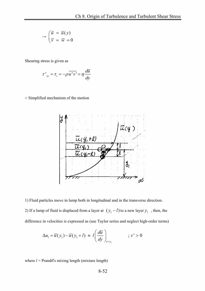
→ ( )
0
u u y
v w
Shearing stress is given as
' ' 'xy t
duu v
dy
○ Simplified mechanism of the motion
1) Fluid particles move in lump both in longitudinal and in the transverse direction.
2) If a lump of fluid is displaced from a layer at 1( )y l to a new layer 1y , then, the
difference in velocities is expressed as (use Taylor series and neglect high-order terms)
1
1 1 1( ) ( ) ; ' 0y y
duu u y u y l l v
dy
where l = Prandtl's mixing length (mixture length)

Ch 8. Origin of Turbulence and Turbulent Shear Stress
8-53
For a lump of fluid which arrives at 1y from the laminar at 1y l
1
2 1 1( ) ( ) ; ' 0y y
duu u y l u y l v
dy
3) These velocity differences 1 2( , )u u caused by the transverse motion can be regarded as
the turbulent velocity fluctuation at 1y
1
1 2
1( )'
2y
duu u lu
dy
(2)
○ Physical interpretation of the mixing length l.
= distance in the transverse direction which must be covered by an agglomeration of fluid
particles travelling with its mean velocity in order to make the difference between it's velocity
and the velocity in the new laminar equal to the mean transverse fluctuation in turbulent flow.
4) Transverse velocity fluctuation 'v originates in two ways.

Ch 8. Origin of Turbulence and Turbulent Shear Stress
8-54
5) Transverse component 'v is same order of magnitude as 'u .
' 'du
v const u const ldy
(3)
6) Fluid lumps which arrive at layer 1y with a positive value of v’ (upwards from layer) give
rise mostly to a negative u’.
' ' 0u v
' ' ' 'u v c u v (4)
where 0 < c < 1
Combine Eqs. 2-4
2' 'du du
u v constant ldy dy
Include constant into l (mixing length)
2' 'du du
u v ldy dy
(5)
Therefore, shear stress is given as
2' 'du du
u v ldy dy
(6)
→ Prandtl's mixing-length hypothesis

Ch 8. Origin of Turbulence and Turbulent Shear Stress
8-55
8.6.3 Von Karman's similarity hypothesis
○Assumptions
∼Turbulent fluctuations are similar at all point of the field of flow (similarity rule).
→ Turbulent fluctuations differ from point to point only by time and length scale factors.
Velocity is characteristics of the turbulent fluctuating motion.
For 2-D mean flow in the x - direction, a necessary condition to secure compatibility between
the similarity hypothesis and the vorticity transport equation is
2 2
/
/
du dyl
d u dy
2 2
/
/
du dyl
d u dy (A)
where = empirical dimensionless constant
Substituting (A) into (8.32) gives
42
2 2 2
( / )
( / )
du dy
d u dy (8.35)
→ Von Karman's similarity rule

Ch 8. Origin of Turbulence and Turbulent Shear Stress
8-56
[Re] Prandtl's velocity-distribution law
For wall turbulence (immediate neighborhood of the wall)
2
2 2 duy
dy
(1)
*1du u
dy y y
(2)
where *u = shear velocity; = von Karman const ≈ 0.4
Integrate (2) w.r.t. y
* lnu
u y C
(3)
→ Prandtl's velocity distribution law
Apply Prandtl's velocity distribution law to whole region
maxu u at y h
*max ln
uu h C
(4)
Subtract (3) from (4) to eliminate constant of integration
max
*
1ln
u u h
u y
(5)
→ Prandtl's universal velocity-defect law

Ch 8. Origin of Turbulence and Turbulent Shear Stress
8-57
Homework Assignment # 5
Due: 1 week from today
8-1. The velocity data listed in Table were obtained at a point in a turbulent flow of sea water.
1) Compute the energy of turbulence per unit volume.
2) Determine the mean velocity in the x -direction u and verify that 'u =0.
3) Determine the magnitude of the three independent turbulent shear stresses in Eq. (8-21).
time,
sec
u
cm/s
'u
cm/s
'v
cm/s
'w
cm/s
0.0 89.92 -4.57 1.52 0.91
0.1 95.10 0.61 0.00 -0.30
0.2 103.02 8.53 -3.66 -2.13
0.3 99.67 5.18 -1.22 -0.61
0.4 92.05 -2.44 -0.61 0.30
0.5 87.78 -6.71 2.44 0.91
0.6 92.96 -1.52 0.91 -0.61
0.7 90.83 -3.66 1.83 0.61
0.8 96.01 1.52 0.61 0.91
0.9 93.57 -0.91 0.30 -0.61
1.0 98.45 3.96 -1.52 -1.22


![Local Wave Number Model for Inhomogeneous Two-Fluid Mixing · ow, with Unstably Strati ed Homogeneous Turbulence (USHT) [22], and shear-driven and buoyancy-driven turbulent ows [19].](https://static.fdocuments.in/doc/165x107/60aa226afcf02805185c46e7/local-wave-number-model-for-inhomogeneous-two-fluid-mixing-ow-with-unstably-strati.jpg)