Optimizing Multiple Object Tracking and Decision making using neuro"“fuzzy
CHAPTER 8 Optimizing multiple objectives under system...
34
167 CHAPTER 8 Optimizing multiple objectives under system of max- Archimedean fuzzy relation equations ______________________________________________________________________________ 8.1 Introduction Optimization is a procedure to hunt for the best solution of a decision problem offering the most suitable alternative available in its domain. Optimization occurs at various levels and stages in real life usage systems whether materialistic or non-materialistic. So a good optimization strategy can affect the overall efficiency of the system. A real life large scale problem involves a wide number of factors and relations amongst them. Due to association and interaction of a large number of components in the system it is impractical to expect the desired accuracy in achieving the preferred goal. The reason behind this is the subjectivity that is accompanied with different components and their interactions. Moreover, it is natural when the interaction amongst the different components results in vagueness. Most often it becomes difficult to neglect the subjectivity that usually appears in their relations. Fuzzy relations offer the appropriate tool to handle this situation when the factors are somehow related or in other words when the relation amongst them are imprecise or not clear. Fuzzy information in relational structures is processed via fuzzy relation equations (FRE). Generally, an optimization problem involves a single objective to be optimized. But dealing with reality it is not rare to face problems that demand a number of objectives to be optimized simultaneously. Such problems are categorized as ‘multiobjective or multicriterion optimization problems (MOOP)’. Moreover, the rise of several conflicting objectives enhances the complexity of the problem, conflicting in the sense that they are negatively correlated. In this case, it is hardly possible to find the solutions that optimize all the objectives together. So, multiobjective optimization generally aims to end up with one or more good compromising solutions for the problem. Hence, the term optimize
Transcript of CHAPTER 8 Optimizing multiple objectives under system...

167
CHAPTER 8
Optimizing multiple objectives under system of max-
Archimedean fuzzy relation equations
______________________________________________________________________________
8.1 Introduction
Optimization is a procedure to hunt for the best solution of a decision problem offering
the most suitable alternative available in its domain. Optimization occurs at various levels
and stages in real life usage systems whether materialistic or non-materialistic. So a good
optimization strategy can affect the overall efficiency of the system. A real life large
scale problem involves a wide number of factors and relations amongst them. Due to
association and interaction of a large number of components in the system it is
impractical to expect the desired accuracy in achieving the preferred goal. The reason
behind this is the subjectivity that is accompanied with different components and their
interactions. Moreover, it is natural when the interaction amongst the different
components results in vagueness. Most often it becomes difficult to neglect the
subjectivity that usually appears in their relations. Fuzzy relations offer the appropriate
tool to handle this situation when the factors are somehow related or in other words when
the relation amongst them are imprecise or not clear. Fuzzy information in relational
structures is processed via fuzzy relation equations (FRE).
Generally, an optimization problem involves a single objective to be optimized. But
dealing with reality it is not rare to face problems that demand a number of objectives to
be optimized simultaneously. Such problems are categorized as ‘multiobjective or
multicriterion optimization problems (MOOP)’. Moreover, the rise of several conflicting
objectives enhances the complexity of the problem, conflicting in the sense that they are
negatively correlated. In this case, it is hardly possible to find the solutions that optimize
all the objectives together. So, multiobjective optimization generally aims to end up with
one or more good compromising solutions for the problem. Hence, the term optimize

168
means finding such a solution which would give the values of all the objective functions
acceptable to the decision maker [114].
The first notion of optimality in this setting goes back to Edgeworth [26] in 1881 and
Pareto [122] in 1896 and is still the most widely used. In this situation, instead of a single
optimal solution usually a set of good, alternative solutions also called as the Pareto
optimal set is obtained. These solutions are optimal in the sense that no other solution in
the search space is better than them when all objectives are considered at the same time.
When the objectives are competing, one objective has to sacrifice for the others and vice-
versa. The situation becomes more complicated when the number of objectives is large.
Although a wide class of methods is available to deal with MOOP but an efficient
procedure is always at demand. So this area of research has always been fascinating for
the researchers.
In the same direction evolutionary techniques or algorithms (EA) have emerged as a
powerful tool to deal these problems efficiently. They have some inherent features to
solve such kind of problems regardless of much mathematical background required.
Evolutionary algorithms perform well even in multimodal, nonlinear search spaces. Due
to this striking characteristic, these algorithms do better than the other optimization
methods used to solve MOOP. Jones et al. [62] reported that 90% of the approaches to
solve multiobjective optimization problems aimed to approximate the true Pareto front
for the underlying problem. A majority of these used a meta-heuristic technique, and 70%
of all metaheuristics approaches were based on evolutionary approaches.
The two general approaches that are used to handle MOOP are: (i). Scalarizing multiple
objectives into a single objective by translating multi-criterion space to single-criterion
space based upon some utility function. This translation requires some prior information
about the problem from the decision maker in terms of some utility function or
predefined preference vector of weights denoting the measures of importance of the
different objectives etc. This method is conceptually straight-forward and
computationally efficient and works well even when the dimension of the criterion space

169
is large. For the practical standpoint a solution close to the solutions in Pareto optimal
front is obtained, representing the most suitable option from the objective space. (ii). The
second general approach is to determine the entire Pareto optimal front or a
representative subset of solutions that are incomparable to each other in terms of the
objectives values. Though the method is a smart way to estimate a set of optimal
solutions for the problem but is computationally challenging and faces difficulty as the
problem size and the number of objectives increase. In addition to it many times the
method struggles to obtain the diverse set of solutions [19]. Some best known population
based Pareto approaches to deal with MOOP are present in [28,29,55,77,159,168]. A
comprehensive survey of all methods to solve MOOP is presented in [16].
The first approach to solve MOOP is generally ignored even if it is efficient and easy to
design because of its sensitivity to the prior inputs it demands to solve the problem. The
entire beauty of this method lies in the efficient incorporation of the prior information to
the problem.
We are considering a fuzzy relational multiobjective optimization problem (FRMOOP)
with the feasible domain designed by a system of fuzzy relational equations. The problem
domain is generally non-convex and the objective functions considered are not
necessarily linear. With a careful observation of the feasible domain, an effective
hybridized genetic algorithm is proposed without determining the complete set of
minimal solutions of system of fuzzy relational equations. The goal of the method is to
generate a set of approximate efficient solutions that allows the decision maker to choose
the best compromising solution.
A great deal of literature has been devoted to the area of multiobjective optimization as it
has always been challenging to deal with numerous objectives having different
characteristics at the same time. In area of fuzzy relational optimization, it is still in
budding stage. Firstly, Wang [182] studied the problem of multiobjective mathematical
programming with multiple linear objective functions subjected to max-min composite
fuzzy relation equation. But the work required the knowledge of all minimal solutions of

170
the system of fuzzy relational equations, which is not trivial at all.
Loetamonphong et al. [90] studied MOOP with multiple objective functions constrained
to a set of max-min fuzzy relational equations. Since the feasible domain of such a
problem is non-convex in general and the objective functions are not necessarily linear,
traditional optimization methods may become ineffective and inefficient. Therefore,
taking advantage of the special structure of the solution set, they developed a reduction
procedure to simplify the problem. Then they proposed a genetic algorithm to find the
Pareto optimal solutions.
Khorram and Zarei [69] considered a multiple objective optimization model subject to a
system of fuzzy relational equations with max-average composition and presented a
reduction procedure in order to reduce problem dimension and then used a modified
genetic algorithm to solve the problem.
Zhang et al. [216] provided an efficient method utilizing a max-pro optimum scheme for
solving the max-min decision function in a fuzzy optimization environment. They
proposed a method significantly simplifying the max-min optimum solving problem,
especially in the case when the number of objectives and constraints is large.
Jiménez et al. [60] considered multiobjective linear programming problem. They
assumed that the decision maker has fuzzy goals for each of the objective functions. In
the case that one of our goals is fully achieved, a fuzzy-efficient solution may not be
Pareto-optimal and proposed a general procedure to obtain a non-dominated solution,
which is also fuzzy-efficient. Further Jiménez and Bilbao [61] proposed that in fuzzy
optimization it is desirable that all fuzzy solutions under consideration are attainable, so
that the decision maker will be able to make a posteriori decisions according to current
decision environments. A case study was analyzed and the proposed solutions from the
evolutionary algorithm considered were given.
Thapar et. al [177] considered a multiobjective optimization problem subjected to a

171
system of fuzzy relational equations based upon the max-product composition. A well
structured nondominated sorting genetic algorithm was applied to solve the problem.
In most of the existing literature, max-min composition or the max-product composition
based fuzzy relational constraints have been discussed. A restriction with max-min
composition is that it is conservative in nature; it has limitations over the application
towards the real world decision problems. It is generally used when a system requires
conservative solutions in the sense that the goodness of one value cannot compensate the
badness of another value [90]. In this paper, we consider the multiobjective optimization
problem with max-Archimedean composition based on an Archimedean t-norm and
propose a hybrid genetic algorithm to determine the set of approximate efficient solutions
of the considered optimization problem.
8.2 The problem
Consider [ ], 0 1,ij ijA a a= ≤ ≤ be a m n× dimensional fuzzy matrix and 1 2[ , , , ],n
b b b b= …
0 1,jb≤ ≤ be a -n dimensional vector. The system of fuzzy relational equations is defined
by A and b as follows:
(8.1)x A b=�
where “ � ” denotes max-� composition of x and A ; � denotes the Archimedean t-
norm operator from the residuated lattice [0,1], , , , , 0,1 .tL = ∧ ∨ Θ� It is intended to find
a solution vector 1 2[ , , , ],m
x x x x= … with 0 1,i
x≤ ≤ such that
1
max ( ) , 1, 2, , (8.2)m
i ij ji
x a b j n=
= ∀ =� …

172
Let {1, 2, , }I m= … and {1, 2, , }J n= … be the index sets. We consider the following
multiobjective optimization model with max-Archimedean fuzzy relational equations as
constraints:
1 1 2 2Min { ( ), ( ), , ( )} (8.3)
s.t. max( ) ,
0 1,
s s
i ij ji I
i
z f x z f x z f x
x a b j J
x i I
∈
= = =
= ∀ ∈
≤ ≤ ∀ ∈
…
�
where ( )k
f x is a linear or nonlinear objective function, {1, 2, , }.k K s∈ = … In this
multiobjective optimization problem, the constraint set is designed by the system of fuzzy
relational equations defined in (8.2).This situation appears in real life optimization
problem whenever the interactions between activities and the resource utilization exhibit
imprecise character.
The characterizations of solution space and consistency conditions have been discussed
in chapters 7. According to [4,49,86], if ( , ) ,X A b φ≠ then in general, it is a non-convex
set which is completely determined by unique maximum solution x�
and possibly finite
number of minimal solutions .x�
The maximum solution is computed explicitly by the
residual implicator (pseudo complement) as:
[min( )] (8.4)t ij t j i I
j Jx A b a b ∈
∈= Θ = Θ�
where sup{ [0,1] | ( ) }ij t j i i ij ja b x x a bΘ = ∈ ≤�
The feasible domain for the problem is given by the union of different convex sub-
feasible regions formed with the help of different minimal solutions say L and the unique
maximal solution .x�
Let { | }p pX x X x x x= ∈ ≤ ≤
� � denotes
thp sub-feasible region given
which is a lattice. The entire solution set ( , )X A b of system (8.2) is given as:
1 2
1( , ) [ , ] [ , ] [ , ] [ , ].
Lp p L
pX A b X x x x x x x x x
== ∪ = ∪ ∪ ∪ ∪ ∪
� � � � � � � �… …

173
Definition 8.2.1. For each ( , ),x X A b∈ we define 1 2( , , ..., )s
x x x xz z z z= to be its criterion
vector where ( ),k
x
kz f x k K= ∈ .
Let us define objective space { ( ) | ( , )}xZ z f x x X A b= = ∈ as the image of the decision
space under the mapping : ( , ) sf X A b R→ where
sR is the s-dimensional Euclidean
space. The image of a solution under this mapping in the objective space is known as the
criterion vector.
Definition 8.2.2. A point ( , )x X A b′∈ is an efficient or a Pareto optimal solution to the
problem (8.3) iff there does not exist any ( , )x X A b∈ such that ( ) ( ), ,k k
f x f x k K′≤ ∀ ∈
and ( ) ( )k k
f x f x′< for at least one k K∈ . Otherwise, x′ is an inefficient solution.
Definition 8.2.3. For any two criterion vectors, 1 2,z z we say that
1z dominates
2z iff
1 2z z≤ and 1 2 1 2 1 2i.e. , andk k k kz z z z k K z z≠ ≤ ∀ ∈ < for at least one .k
Definition 8.2.4. z Z′∈ is said to be nondominated iff there does not exist any z Z∈
that dominates ,z′ otherwise z′ is a dominated criterion vector.
The set of all efficient solutions is called as the efficient set and the image of the efficient
set in objective space is the nondominated set.
Definition 8.2.5. The criterion vector z∗composed of the least attainable objective
function values in the problem domain is called the ideal point i.e. k K∀ ∈
{ | min( ( )), }k k k kz z z z x x X∗ = = ∈
In general, the concept of ideal point is impractical and it corresponds to a non-existent
solution. But it plays an important role in numerous methods used to solve MOOP [18].

174
Definition 8.2.6. An objective vector z∗∗
formed with components slightly less than that
of the ideal objective vector is known as the utopian objective vector i.e. k k kz z ε∗∗ ∗= −
with 0k
ε > , k K∀ ∈ .
8.3 Utility function approach for MOOP
The utility function approach has always been the favorite and simple technique to solve
the multicriterion optimization problems due to the lesser complexity involved.
Moreover, it is hardly possible to determine the solutions that optimize all the objectives
together. A utility function : sU R R→ is a mathematical representation of decision
maker’s preferences mapping criterion vectors into the real line giving a value of utility
for decision maker. It is used as an approximation of the preference function of the
decision maker that typically cannot be expressed mathematically. Basically, the utility
function combines given multiple objectives into a single objective function by
incorporating the prior information supplied by the decision maker about the problem.
Using the utility function the problem defined in (8.3) transforms to the following
mathematical programming problem:
1 2Minimize ( ( ), ( ),..., ( )) (8.5)
s.t. ( , )
sU z x z x z x
x X A b∈
Multiple objectives can be combined into a single objective in many ways. Different
utility functions have been studied in the literature in this field [18,96,97,101,171]. The
most general utility functions that are used in literature are weighted metric utility
function and weighted linear utility function, weighted exponential sum, weighted
product, weighted max etc. The transformed fuzzy relational optimization problems
based on some of these utility functions are described as follows:

175
8.3.1 Weighted linear utility function
This method linearly combines different objectives to a scalarized single objective as
follows:
1
( ) ( )s
k k
k
Z x f xλ=
=∑
s.t. ( , )x X A b∈
where ( )k
f x is the thk objective function with the weight vector 1 2
( , ,..., ) ,s
λ λ λ λ=
meeting the following conditions1
0, 1; for .s
k k
k
k Kλ λ=
> = ∈∑
i.e., the aggregated function to be optimized is the convex combination of all the
objectives under considerations. This is the most widely studied and simple kind of utility
function that is used. Generally, the weights represent the relative importance of the
objectives. The success of the method lies in the efficient determination of weights for
the objectives. A detailed analysis of this method is presented in the work
[97,101,171].This method works well as far as convex multiobjective optimization
problems are concerned but lacks sometimes in finding certain Pareto optimal solutions
in case of non-convex MOOP.
Theorem 8.3.1.[101]. The solution to the problem presented in equation (8.5) is Pareto-
optimal iff the weight is positive for all objectives i.e. 0, .k
k Kλ > ∀ ∈
Besides its powerful qualities the method also suffers from some drawbacks. One is the
scaling of objectives that is required while selecting the weights. As different objectives
might attain values of different orders, scaling of objectives must be performed before
aggregation so that each objective could have magnitude of same order. Secondly, while
handling mixed kind of objectives all objectives need to be converted to the same type
using the duality principle as discussed in [18].

176
8.3.2 Weighted metric utility function
This method presents another approach of combining multiple objectives via the distance
minimization of the particular solution from the ideal point based on different metrics. In
this method, for a non-negative weight vector the utility function using the distance
measure based on p-metric is considered as follows:
1/
1
( ) ( | ( ) | )s
p p
p k k k
k
Z x f x zλ ∗
=
= −∑
s.t. ( , )x X A b∈
Where (1, )p ∈ ∞ is the distance metric and z∗ is the ideal point. When 1,p = the
resulting problem is equivalent to the weighted sum approach. For 2,p = the Euclidean
distance is minimized. When ,p = ∞ the metric is also known as the Tchebycheff metric
and the transformed utility function has a special name as Weighted Tchebycheff
function given as:
1( , , ) max{ | ( ( ) ) |}
s
k k kk
Z z z f x zλ λ∗ ∗∗∞
== −
where 1 2( , ,..., ) 0,
s kλ λ λ λ λ= ∀ ≥ and z
∗∗is the reference point. When the Tchebycheff
metric is used, each and every Pareto optimal solution of the considered MOOP can be
found if the utopian point is used as the reference point [101,171]. For each efficient
solution there exists a weighted Tchebycheff scalarizing function such that it is global
optimum (minimum) of the considered MOOP. By altering the weight vector at each run,
the entire Pareto optimal set can be obtained. Alike the weighted sum approach this
method also requires the scaling of objectives before combining them due to the same
reason as mentioned in case of linear utility function. Moreover, the method is sensitive
to the choice of the metric being used and might not be suitable in case of continuous
MOOP as the aggregating function is not continuous in nature.

177
It is noteworthy that all weighted Tchebycheff utility functions have optima in the
nondominated set and vice-versa. Thus, finding the whole nondominated set is same as
finding optima of all weighted Tchebycheff scalarizing functions. Hence, we reconsider
the problem (8.3) as optimization of different weighted Tchebycheff scalarizing
functions. In fact, it is enough to consider different weighted Tchebycheff scalarizing
functions with normalized weight vectors. Each efficient approximate solution is the
global optima of the current weighted utility function.
8.3.3 Weighted- product utility function
To allow functions with different orders of magnitude to have similar significance and to
avoid having to transform objective functions, one may consider the following
formulation:
1
( ) [ ( )] k
s
k
k
Z x f xλ
=
= ∏
s.t. ( , )x X A b∈
where 1 2( , ,..., ) 0,
s kλ λ λ λ λ= ∀ ≥ are weights denoting the relative importance of the
objectives. All these described methods and many more [18,96] based on the aggregation
of objectives require prior knowledge about the problem in terms of the aggregating
coefficients.
8.4 Multiobjective hybrid genetic algorithm (MOHGA)
In multiobjective optimization the focus is on generating the entire efficient solution set
to support decision making. This set of solutions allows the decision maker to choose a
good compromise solution for the practical purpose. The computational complexity of
MOOP directs the use of metaheuristics as the most promising method to solve them. In
recent years, hybridized evolutionary algorithms have been proved as a potent technique
to solve MOOP, as they offer more competencies and result in much diversified solution
178
set. The method possesses a combined effect of recombination operators and local search
scheme. They are also known as the genetic local search or memetic algorithm. Different
aspects of hybrid genetic algorithms and some of its applications are discussed in [56-58].
A great deal of literature available for solving MOOP discusses the application of genetic
algorithm. A hybrid evolutionary algorithm with local search for multiobjective
optimization was first implemented by Ishibuchi and Murata [58].The goal of multiple
objective metaheuristics is to generate good approximations to the nondominated set. Of
course, the true approximation is the whole nondominated set itself. The multiobjective
hybridized genetic algorithm (MOHGA) that we are developing; performs the
simultaneous optimization of all aggregated functions constructed by the weighted sum
approach or weighted Tchebycheff approach. At each run, a randomly generated
aggregated objective is optimized that results in an approximate solution belonging to the
set of efficient solutions. A hybrid genetic algorithm is used to optimize each of the
weighted utility function considered. The evolutionary procedure that we are applying to
solve (8.5) is described as follows:
8.4.1 Initialization
The feasible domain for the considered problem has a special structure. As the feasible
region is designed by a system of fuzzy relational equations, it might be the case that
some of the variables assume specific value. So it is good to perform elementary
reduction first to reduce the problem size.
With the help of computed maximum solution x�
, the characteristic matrix ( )ij m nM m ×=
of the system x A b=� is defined as:
[( ), ], if ( )(8.6)
otherwise
ij t j i i ij j
ij
a b x x a bm
θ
φ
==
� ��

179
[ ]where inf{ 0,1 | ( ) } , [0,1]ta b z z a b a bθ = ∈ ≥ ∀ ∈� .Each element ijm of characteristic
matrix M offers all the possible values for the variable ix to satisfy the
thj equation. The
system x A b=� is consistent if and only if M has no column with all elements as empty
elements i.e. every equation is satisfied by at least one variable.
The characteristic matrix M of A is further simplified to a binary matrix M as follows:
1 if(8.7)
0 otherwise
ij
ij
mm
φ ≠=
Note that the entry 1ijm = in M corresponds to a possible selection of the thi variable
that satisfies the th
j equation.
Now 0, ,jb j J∃ = ∈ its corresponding column in M and the corresponding component
from b can be removed. A variable is said to be pseudo-essential if the row
corresponding to it has only empty elements in the characteristic matrix M of A. Such
variables satisfy only those equations for which 0.jb = It is clear that the role of pseudo-
essential variable is trivial. So, its corresponding row from M can be removed.
Definition 8.4.1. For column ,j J∈ if there is only one i I∈ such that 1ijm = then
variable i i ix x x= =� �
is called super-essential for all ( , ).x X A b∈
For the sake of solvability of the system the presence of super-essential variables is must
in all the solutions. To reduce the size of the problem, other equations that are satisfied by
these variables, can also be exempted for further computation.
Once the pseudo-essential variables have been detected and super-essential variables are
fixed, the size of the system reduces. The whole reduction procedure used is explained
via the following example.
180
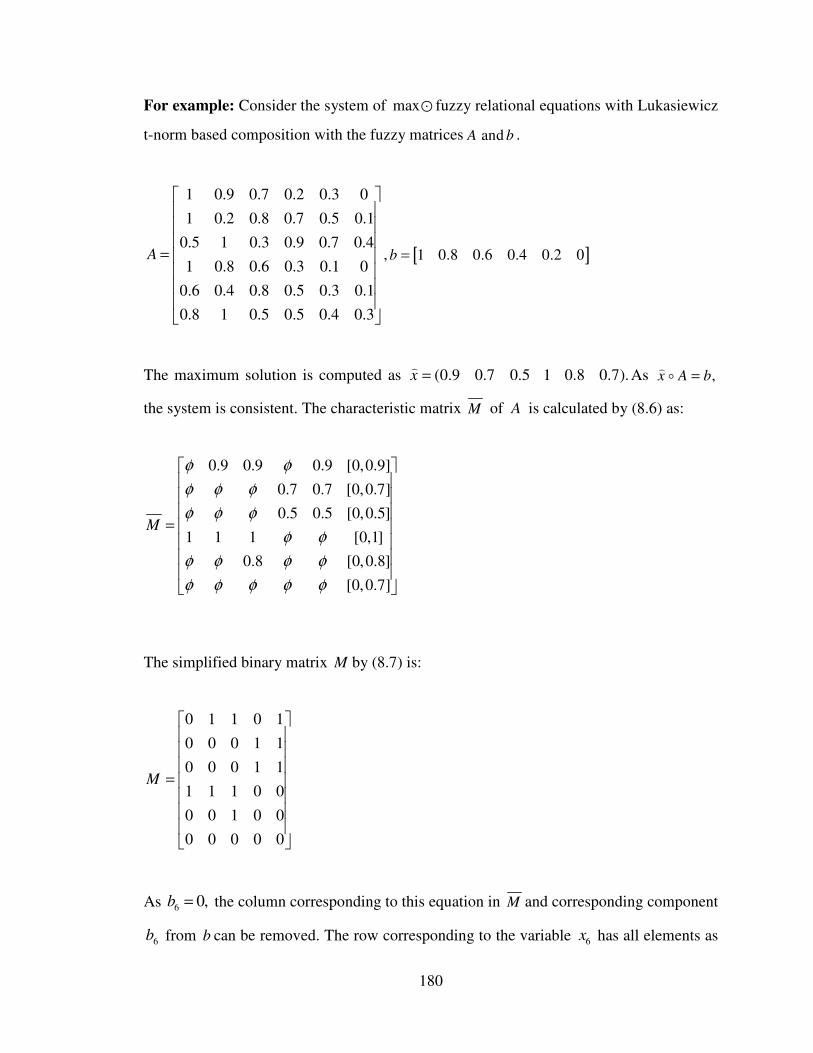
For example: Consider the system of max� fuzzy relational equations with Lukasiewicz
t-norm based composition with the fuzzy matrices andA b .
1 0.9 0.7 0.2 0.3 0
1 0.2 0.8 0.7 0.5 0.1
0.5 1 0.3 0.9 0.7 0.4
1 0.8 0.6 0.3 0.1 0
0.6 0.4 0.8 0.5 0.3 0.1
0.8 1 0.5 0.5 0.4 0.3
A
=
, [ ]1 0.8 0.6 0.4 0.2 0b =
The maximum solution is computed as (0.9 0.7 0.5 1 0.8 0.7).x =�
As ,x A b=��
the system is consistent. The characteristic matrix M of A is calculated by (8.6) as:
The simplified binary matrix M by (8.7) is:
0 1 1 0 1
0 0 0 1 1
0 0 0 1 1
1 1 1 0 0
0 0 1 0 0
0 0 0 0 0
M
=
As 60,b = the column corresponding to this equation in M and corresponding component
6b from b can be removed. The row corresponding to the variable 6
x has all elements as
0.9 0.9 0.9 [0,0.9]
0.7 0.7 [0,0.7]
0.5 0.5 [0,0.5]
1 1 1 [0,1]
0.8 [0,0.8]
[0,0.7]
M
φ φ
φ φ φ
φ φ φ
φ φ
φ φ φ φ
φ φ φ φ φ
=

181
zeros in ,M the variable 6x is pseudo-essential and can be excluded for further
computation. The first equation is satisfied by only variable 4,x 4
x is super-essential and
is fixed to be 4 4x x=�
in all solutions. Variable 4x also satisfies second and third
equations, so these equations can also be exempted for further computation. This reduces
the problem to x A b′ ′=� where
0.2 0.3
0.7 0.5
0.9 0.7
0.3 0.1
0.5 0.3
0.5 0.4
A
′ =
, [ ]0.4 0.2b′ =
For the sake of solvability of FRE the random generation of population is not feasible as
it might result in unnecessary exploration of the search space. Firstly, the super-essential
variables have been detected and their values are fixed as i ix x=�
. An initial population of
fixed size is created with the fixed variables assuming the value ix�
and the variables that
are not fixed assuming a random value in the range (0 ).i
x�
Each solution
1 2( , ,..., )
mx x x x= is the member of ( , ).X A b Now the feasibility of generated solutions is
examined. The following algorithm has been used to maintain the feasibility of the
solutions:
Algorithm 1: For maintaining feasibility of solutions
Step 1: Choose a violated constraint j . Let { | }j ij jD i I a b= ∈ ≥ .
Step 2: Randomly choose an element .jk D∈ For kj ja b> or ,k kj t jx a b= Θ
� set
.k kj t jx a b= Θ Otherwise, assign a random number between [( ), ]kj t j ka b xΘ�
to .k
x
Step 3: Check the feasibility of the new solution. If the solution is feasible stop else go to
step 1 and repeat the process.

182
8.4.2 Selection
Once the initial population has been generated, selection of good individuals is the next
step to apply the recombination operator. The selection of good individuals at this step is
performed via the rank selection scheme. The individuals are evaluated using the current
utility function for that particular run. A normalized weight vector giving a new utility
function is randomly selected for each run.
The probability of selection for each individual is determined by the following formula:
1
11
max( ( )) ( )( ) , 1, 2,...,
( ) max( ( ))
Nt t
t t
N Nt t
it
z x z xp x t N
z x z x
=
==
−= =
−∑
where ( )tz x denotes the fitness of the th
t individual with respect to the objective function
defined with the current weight vector for that run and N is the population size. A pre-
specified number of parent solutions are selected at the end. Selected individuals undergo
the recombination process so as to create a new population by using genetic operators
crossover and mutation.
8.4.3 Crossover
Owing to the nature of solution space of the problem, the conventional real coded
crossover techniques are not feasible. A domain specific crossover scheme is designed
that generates feasible individuals. The algorithm used for crossover can be described in
the following steps:
Algorithm 2: Crossover
Get the matrices ,A b and find the maximum solution x�
by (8.4) and set parameters
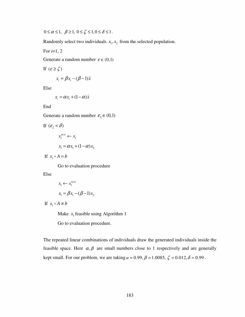
183
0 1,α≤ ≤ 1,β ≥ 0 1, 0 1ζ δ≤ ≤ ≤ ≤ .
Randomly select two individuals 1 2,x x from the selected population.
For i=1, 2
Generate a random number (0,1)ε ∈
If ( )ε ζ≥
( 1)i i
x x xβ β= − −�
Else
(1 )i i
x x xα α= + −�
End
Generate a random number 2(0,1)ε ∈
If 2( )ε δ<
1 1
nextx x←
1 1 2(1 )x x xα α= + −
If 1x A b=�
Go to evaluation procedure
Else
1 1
nextx x←
1 1 2( 1)x x xβ β= − −
If 1x A b≠�
Make 1x feasible using Algorithm 1
Go to evaluation procedure.
The repeated linear combinations of individuals draw the generated individuals inside the
feasible space. Here ,α β are small numbers close to 1 respectively and are generally
kept small. For our problem, we are taking 0.99, 1.0085, 0.012, 0.99α β ζ δ= = = = .

184
8.4.4 Mutation
Mutation randomly perturbs a candidate solution by exploiting the search space with a
hope to create a better solution in the problem domain. We adopt the following mutation
procedure to solve our problem:
Algorithm 3: Mutation
Step 1: Get the matrices ,A b and find the maximum solution x�
by (8.4) and set the
mutation probability 0.1.δ =
Step 2: Generate random number (0,1)i
r ∈ for each bit of the individual selected from
crossed population.
Step 3: For i I∈ , if ir δ≤ , randomly assign i
x a number from (0, )i
x�
.
Step 4: For the modified 1 2( , ,..., )
mx x x x= check feasibility x A b=� . If x A b=� go to
the evaluation procedure else make the individual feasible via Algorithm 1.
The operator is designed such that the mutated individuals remain feasible. The mutation
probability 0.1δ = has been used i.e. each component of all the solution vectors has 10
percent chances of being mutated.
Apart from the general structure of GA, the procedure also keeps track of the non-
dominated solutions. This feature of the procedure differentiates it from the traditional
metaheuristics used to solve MOOP. For this the nondominated solutions in the initial
population having good ranks are identified and their replicates are maintained separately
for that current population as the secondary population. To determine the rank of a
solution concept of domination, as explained through Definitions 8.2.1-8.2.4 has been
used. The rank ,pr of an individual p is determined by the number of dominators or
solutions whose criterion vectors dominate this individual’s criterion vector. It is defined
as,
number of dominators, 1, 2, , .pr N p N= − = …

185
The probability of selection of an individual with rank pr is given by
1
p
N
i
i
r
r=
∑
Once new solutions are obtained after the recombination process a pre-specified number
of nondominated solutions (the elite solutions) are randomly selected from the secondary
population and added to the newly generated solutions.
8.4.5 Local search scheme
The combined population formed after the recombination operators along with the elite
nondominated solutions selected from the secondary population undergoes the local
search operation. While applying the local search scheme it is necessary to maintain the
balance between the local search and the genetic search. The imbalance in the two can
cause the unfruitful exploration of the search space that in turn increases the time to run
the algorithm. When local search is applied to a solution, a random new point is selected
from the neighborhood of the current point. We consider the neighborhood ( 0.05, 0.05)−
of radius 0.05 . If the new solution provides a better value of the current utility function
for that run, the selected solution is replaced by the current solution. Otherwise, some
other neighbor is selected and tested against the current solution. To decrease the CPU
time spent on the local search, the number of solutions examined in neighborhood of a
solution is pre-fixed. The method terminates if no further improvement is possible until
the number of successive fails to examine the improved solution ends up. If no improved
solution is obtained the initial solution is kept as such in the population. This procedure is
repeated for all the solutions in the population that undergo the local search procedure.
The local search operator by its nature is capable of improving the scalar objective
formed. But the selection of individuals for local search is a crucial step to be emphasized
on. The choice of the individuals for local search can be done in one of the following
ways [145]:
Hybrid strategy # 1: Selecting some fixed number of nondominated solutions according

186
to their domination rank in that generation.
Hybrid strategy #2: Choose a number of individuals by assigning a probability using
some selection operator.
Hybrid strategy #3: Selecting individuals based on some assigned probability are chosen
in a purely random fashion.
Ishibushi and Murata [58] applied the hybrid strategy#2 for the multiobjective TSP
problem. The overall procedure applied to solve problem (8.5) can be described in
Algorithm 4 as:
Algorithm 4: MOHGA procedure
Step 1: After reducing the size of the problem and fixing the variables, generate the initial
population of sizepN .
Step 2: Extract the nondominated solutions determined in the current population as
secondary population.
Step 3: Select N good solutions from the current population and apply genetic operators,
crossover using Algorithm 2 and mutation using Algorithm 3 on the selected solutions.
Step 4: Randomly select pN N− solutions from the secondary population and add to the
newly generated population in step 3 and combine them to form the final population of
sizepN .
Step 5: Apply local search probabilistically to each of the solution in the final population.
Step 6: Go to step 1 if the termination condition is not satisfied.
The above algorithm repeats for 100 generations to optimize the pre-defined no. of
considered utility functions based on a different weight vector for each run. Figure 8.1
shows the whole procedure of the Algorithm 4 used to solve FRMOOP in (8.5).

187
Figure 8.1: Flow chart of MOHGA procedure
8.5 Results and discussions
In this section, results of the proposed genetic algorithm for multiple linear and nonlinear
optimization problems are discussed. We consider few examples of multiobjective linear
and nonlinear optimization problems and systems of fuzzy relational equations with
different Archimedean t-norm based compositions. We are using the problems with
objectives attaining values of same order so scaling of objectives is not required. The
nature of the solutions obtained using the proposed procedure is investigated. The results
Initialize population of size p
N
Determine nondominated solutions in the current generation
Select good individuals
Apply crossover using Algorithm 2
If termination
condition meet
Start
Apply mutation using Algorithm 3
Yes
Stop
No
gen
=g
en+
1
Ad
d e
lite
so
luti
on
s
Apply local search scheme

188
are compared with the results obtained using the modified NSGA-II1.
In our computational experiments of this paper, we used the following parameter settings:
Population sizepN : 60
Mutation probabilityδ : 0.1
No. of nondominated solutions selected for each iteration n: 15
No. of successive fails for testing local search operator: 20
The experimental results for 6 test problems have been presented graphically from figures
8.2-8.16.
Example 8.1. Consider a four dimensional problem with fuzzy matrices A and b with
max-product composition which is one type of Archimedean t-norm based compositions.
0.5042 0.0569 0.3641 0.2527
0.9398 0.6578 0.0359 0.1663, [0.6120 0.4284 0.8075 0.1083]
0.4979 0.3937 0.5715 0.9849
0.7182 0.0330 0.9476 0.1271
A b
= =
The maximum solution obtained using (8.4) is [0.4286 0.6512 0.1100 0.8521] .For
this particular problem, the values of 2x and 4
x of all solution vectors have to be fixed at
0.6512 and 0.8521 respectively. Therefore, we can focus on values of 1x and 3
x only and
the problem dimension reduces to two. The test results for some multiple linear and
nonlinear optimization problems with this system of fuzzy relational equations as
constraints are discussed below.
1 1 2 3 4
2 1 2 3 4
( ) 2 2 4 ,Case 1. min
( ) 2 3 9 .
f x x x x x
f x x x x x
= + + +
= − − −
The plot of the objective functions against Pareto optimal solutions describe the Pareto
front (PF) or nondominated set. Figure 8.2 shows the set of approximate nondominated
solutions obtained by optimizing 200 randomly selected weighted Tchebycheff functions
and weighted linear functions using MOHGA procedure.
1The modified NSGA-II is described in the Appendix B attached at the end of the thesis.

(a): Results with local search st
(c): Results with local search strategy #3
Figure 8.2: PF obtained using MOHGA
Figure 8.3: PF
4.7 4.75 4.8 4.85-9.75
-9.72
-9.69
-9.66
-9.63
-9.6
Objective f1
Ob
jecti
ve f
2
Weighted Tchebyecheff
function
Weighted linear function
4.7 4.75 4.8 4.85-9.75
-9.72
-9.69
-9.66
-9.63
-9.6
Objective f1
Ob
jecti
ve f
2
Weighted Tchebyecheff
function
Weighted linear function
Ob
ject
ive f
2
189
(a): Results with local search strategy #1 (b): Results with local search strategy #
(c): Results with local search strategy #3 (d): Results without local search strategy
obtained using MOHGA procedure-Example 8.1
PF obtained using modified NSGA-II-Example 8.1
4.85 4.9 4.95Objective f1
Weighted Tchebyecheff
function
Weighted linear function
4.7 4.75 4.8 4.85-9.75
-9.72
-9.69
-9.66
-9.63
-9.6
Ob
jecti
ve
f2
Objective f1
Weighted Tchebyecheff
function
Weighted linear function
4.85 4.9 4.95Objective f1
Weighted Tchebyecheff
function
Weighted linear function
4.7 4.75 4.8 4.85-9.75
-9.7
-9.65
-9.6
-9.55
-9.5
Ob
jecti
ve f
2
Objective f1
4.7 4.75 4.8 4.85 4.9 4.95-9.74
-9.72
-9.7
-9.68
-9.66
-9.64
-9.62
Objective f1
Ob
ject
ive f
2
(b): Results with local search strategy # 2
(d): Results without local search strategy
Example 8.1-Case 1
Example 8.1-Case 1
4.9 4.95
Weighted Tchebyecheff
Weighted linear function
4.85 4.9 4.95Objective f1
Weighted
Tchebeycheff
function
Weighted linear
function

Case 2: 1 1 3
2 1 3
( ) 10( 0.45) 10( 0.35) ,min
( ) 6( 0.7) 10( 0.45) .
f x x x
f x x x
= − + −
= − − + −
Figure 8.4 shows the nondominated set obtained using the proposed approach
modified NSGA-II.
(a) PF obtained with
Figure 8.4: PF obtained using MOHGA
Example 8.2. Consider a five dimensional problem with fuzzy matrices
max-product composition:
0.6733 0.5589 0.2222 0.7631
0.0724 0.5040 0.0345 0.8572
0.1731 0.8747 0.0050 0.2317
0.6095 0.3837 0.0617 0.6200
0.6277 0.68
A =
47 0.2072 0.9481 0.3522
[0.6090 0.7541 0.2010 0.9199 b
=
The maximum solution is obtained as
0.5 1 1.5-2
-1.5
-1
-0.5
0
0.5
1
Objective f1
O
bje
ctiv
e f
2
Weighted Tchebycheff function
Weighted linear function
190
2 2
1 1 3
2 2
2 1 3
( ) 10( 0.45) 10( 0.35) ,
( ) 6( 0.7) 10( 0.45) .
f x x x
f x x x
= − + −
= − − + −
shows the nondominated set obtained using the proposed approach
with MOHGA (b) PF obtained with modified
obtained using MOHGA and modified NSGA-II -Example 8.1
Consider a five dimensional problem with fuzzy matrices
product composition:
0.6733 0.5589 0.2222 0.7631 0.6683
0.0724 0.5040 0.0345 0.8572 0.2942
0.1731 0.8747 0.0050 0.2317 0.4581
0.6095 0.3837 0.0617 0.6200 0.6049
47 0.2072 0.9481 0.3522
[0.6090 0.7541 0.2010 0.9199 0.6044]
The maximum solution is obtained as[0.9044 1.0000 0.8621 0.9992
2 2.5 3 Objective f1
Weighted Tchebycheff function
Weighted linear function
0.5 1 1.5 2-2
-1.5
-1
-0.5
0
0.5
1
Objective 1
Ob
jecti
ve 2
shows the nondominated set obtained using the proposed approach and
modified NSGA- II
Example 8.1-Case 2
Consider a five dimensional problem with fuzzy matrices A and b with
[0.9044 1.0000 0.8621 0.9992 0.9701] . The
2.5 3

values of variables 3x and
0.9701 respectively. Therefore, we can focus only on the values of variables
The test results for a multiple
fuzzy relational equations as constraints are discussed below.
1 1 2 3 4 5
2 1 2 3 4 5
3 1 2 3 4 5
( ) 3 9 4 ,
min ( ) 3 9 4 ,
( ) 3 8 5 6 .
f x x x x x x
f x x x x x x
f x x x x x x
= − − + − −
= + − − + = + − + +
(a). PF obtained with local search
Figure 8.5: PF
Figure 8.6:
-20-16
-120
48
1216
200
3
6
9
12
15
f1f2
f3
Weighted Tchebyecheff function
Weighted linear function
f3
191
and 5x of all solution vectors have to be fixed at 0.8621 and
0.9701 respectively. Therefore, we can focus only on the values of variables
The test results for a multiple objective linear optimization problem with this system of
fuzzy relational equations as constraints are discussed below.
1 1 2 3 4 5
2 1 2 3 4 5
3 1 2 3 4 5
( ) 3 9 4 ,
min ( ) 3 9 4 ,
( ) 3 8 5 6 .
f x x x x x x
f x x x x x x
f x x x x x x
= − − + − −
= + − − +
= + − + +
with local search (b). PF without with
PF obtained with and without local search-Example 8.2
: PF obtained using modified NSGA-II –Example 8.2
-12-8
-40
f1
Weighted Tchebyecheff function
Weighted linear function
-20-16
-12-8
04
812
1620
0
4
8
12
15
f1f2
f3
Weighted Tchebyecheff function
Weighte linear function
-20-16
-12-8
-40
04
812
1620
0
3
6
9
12
15
f1f2
f3
of all solution vectors have to be fixed at 0.8621 and
0.9701 respectively. Therefore, we can focus only on the values of variables 1x , 2
x and 4x .
linear optimization problem with this system of
with local search
Example 8.2
Example 8.2
-8-4
0
f1
Weighted Tchebyecheff function
Weighte linear function

Example 8.3. Consider a problem with fuzzy matrices
composition:
0.7037 0.1254 0.3557 0.2861
0.5221 0.0930 0.0490 0.2512
0.7552 0.1345 0.7553 0.9327
0.4785 0.0852 0.8948 0.1310
A
b
=
= [0.4551 0.0811 0.8511 0.5620
The maximum solution is obtained as
3x and 4
x are super-essential so their values have to be fixed at 0.6026 and 0.9511,
respectively in all solution vectors. Therefore, we can focus on
results for some multiobjective optimizatio
this system of fuzzy relational equations as constraints are discussed below.
1 1 2 3 4
2 2
2 1 2 3 4
5 3
2 3 1 4
( ) 0.3 2 ,
min ( ) ( 2 ) 0.75( )
( 2 ) 0.3( ) .
f x x x x x
f x x x x x
x x x x
= − − +
= − + − + − + −
Figure
1-4
-2
0
2
4
Obje
ctiv
es
f1,f
2
192
Consider a problem with fuzzy matrices A and b with max
0.7037 0.1254 0.3557 0.2861 0.4937
0.5221 0.0930 0.0490 0.2512 0.3663
0.7552 0.1345 0.7553 0.9327 0.5299
0.4785 0.0852 0.8948 0.1310 0.2093
[0.4551 0.0811 0.8511 0.5620 0.3193]
The maximum solution is obtained as[0.6467 0.8717 0.6026 0.9511]
essential so their values have to be fixed at 0.6026 and 0.9511,
respectively in all solution vectors. Therefore, we can focus on 1x and
results for some multiobjective optimization problem with mixed objectives subjected to
this system of fuzzy relational equations as constraints are discussed below.
1 1 2 3 4
2 2
2 1 2 3 4
5 3
2 3 1 4
( ) 0.3 2 ,
min ( ) ( 2 ) 0.75( )
( 2 ) 0.3( ) .
f x x x x x
f x x x x x
x x x x
= − − +
= − + − +
− + −
Figure 8.7: Surface plots of function in Example 8.3
00.2
0.40.6
0.81
00.2
0.40.6
0.81
-4
-2
0
2
4
x1x2
with max-product
[0.6467 0.8717 0.6026 0.9511] . The variables
essential so their values have to be fixed at 0.6026 and 0.9511,
2x only. The test
n problem with mixed objectives subjected to
this system of fuzzy relational equations as constraints are discussed below.

(a): Results with local search
(c): Results with local search strategy #3 (d): Results without using local search
Figure 8.8: PF
Figure 8.9:
0.4 0.6 0.8-3
-2
-1
0
1
2
3
Objective f1
Ob
jecti
ve f
2
Weighted Tchebyecheff function
Weighted linear function
0.4 0.6 0.8-3
-2
-1
0
1
2
3
Objective f1
Ob
jecti
ve f
2
Weighted Tchebyecheff
function
Weighted linear function
193
(a): Results with local search strategy #1 (b): Results with local search strategy # 2
(c): Results with local search strategy #3 (d): Results without using local search
PF obtained using MOHGA procedure -Example 8.3
: PF obtained using modified NSGA-II –Example 8.3
1 1.2 1.4Objective f1
Weighted Tchebyecheff function
Weighted linear function
0.4 0.6 0.8 1-3
-2
-1
0
1
2
3
Objective f1
Ob
jecti
ve f
2
Weighted Tchebyecheff
function
Weighted linear function
1 1.2 1.4Objective f1
Weighted Tchebyecheff
function
Weighted linear function
0.4 0.6 0.8 1-3
-2
-1
0
1
2
3
f1
f2
Weighted Tchebyecheff functionWeighted linear function
0.4 0.6 0.8 1 1.2 1.4-3
-2
-1
0
1
2
3
Objective f1
Ob
jecti
ve f
2
Ob
ject
ive
strategy #1 (b): Results with local search strategy # 2
(c): Results with local search strategy #3 (d): Results without using local search
Example 8.3
Example 8.3
1.2 1.4Objective f1
Weighted Tchebyecheff
Weighted linear function
1.2 1.4
Weighted Tchebyecheff functionWeighted linear function
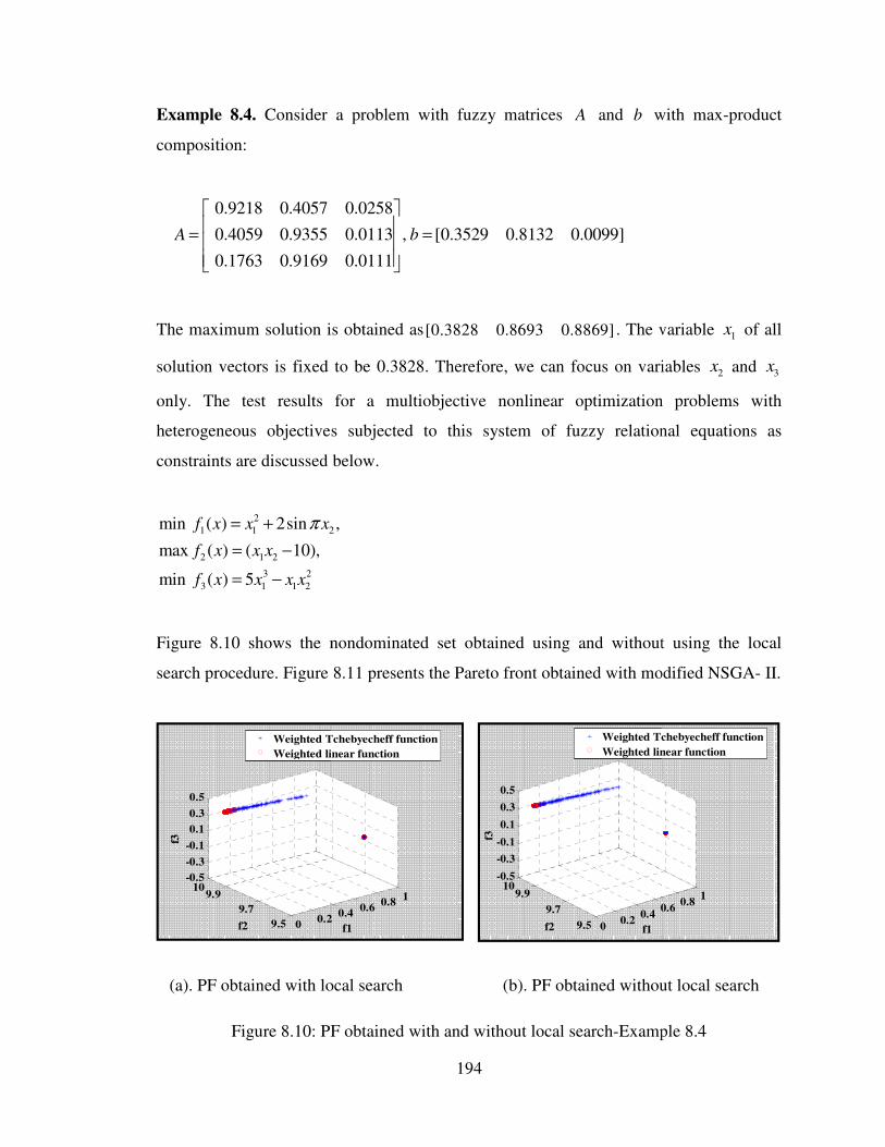
Example 8.4. Consider a problem with fuzzy matrices
composition:
0.9218 0.4057 0.0258
0.4059 0.9355 0.0113 , [0.3529 0
0.1763 0.9169 0.0111
A b
= =
The maximum solution is obtained as
solution vectors is fixed to be 0.3828. Therefore, we can focus on variables
only. The test results for
heterogeneous objectives subjected to this system of fuzzy relational equations as
constraints are discussed below.
2
1 1 2
2 1 2
3 2
3 1 1 2
min ( ) 2sin ,
max ( ) ( 10),
min ( ) 5
f x x x
f x x x
f x x x x
π= +
= −
= −
Figure 8.10 shows the nondominated set obtained using
search procedure. Figure
(a). PF obtained with loca
Figure 8.10: PF
00.2
9.5
9.7
9.910
-0.5
-0.3
-0.1
0.1
0.3
0.5
f2
f3
Weighted Tchebyecheff function
Weighted linear function
194
Consider a problem with fuzzy matrices A and b with max
0.9218 0.4057 0.0258
0.4059 0.9355 0.0113 , [0.3529 0.8132 0.0099]
0.1763 0.9169 0.0111
A b
= =
The maximum solution is obtained as[0.3828 0.8693 0.8869] . The variable
solution vectors is fixed to be 0.3828. Therefore, we can focus on variables
only. The test results for a multiobjective nonlinear optimization problems with
heterogeneous objectives subjected to this system of fuzzy relational equations as
constraints are discussed below.
1 1 2min ( ) 2sin ,
max ( ) ( 10),
f x x x
shows the nondominated set obtained using and without using
8.11 presents the Pareto front obtained with modified NSGA
(a). PF obtained with local search (b). PF obtained without local search
PF obtained with and without local search-Example 8.4
0.20.4
0.60.8
1
f1
Weighted Tchebyecheff function
Weighted linear function
00.2
0.40.6
9.5
9.7
9.910
-0.5
-0.3
-0.1
0.1
0.3
0.5
f1f2
f3
Weighted Tchebyecheff function
Weighted linear function
with max-product
he variable 1x of all
solution vectors is fixed to be 0.3828. Therefore, we can focus on variables 2x and 3
x
nonlinear optimization problems with
heterogeneous objectives subjected to this system of fuzzy relational equations as
and without using the local
Pareto front obtained with modified NSGA- II.
without local search
Example 8.4
0.60.8
1
Weighted Tchebyecheff function
Weighted linear function

Figure 8.11:
Example 8.5. Consider a problem with fuzzy matrices
Hamacher fuzzy relation equations with
Archimedean t-norm:
0.6 0.2 0.3 0.84 0.6 0.12
0.2 0.7 0.1 0.7 0.2 0
0.8 0 0.2 0.7 0.8 0
1 0.6 0.4 0.6 0.5 0.1
A
=
The maximum solution can be obtained by using (
min ( ) where ij t j ij t jj J i I
x a b a b∈ ∈
= Θ Θ =
�
The maximum solution is obtained as
1x and 2
x of all solution vectors are fixed at 0.3750 and 0.4828 respectively. Therefore,
we look for the values of variables
objectives linear optimization problem subjected to this system of fuzzy relational
equations as constraints are discussed as follows:
f3
195
: PF obtained using modified NSGA-II –Example 8.4
Consider a problem with fuzzy matrices A and b composed of max
Hamacher fuzzy relation equations with ( ) ,x a
x ax a x a
⋅=
+ − ⋅� which is one type of the
0.6 0.2 0.3 0.84 0.6 0.12
0.2 0.7 0.1 0.7 0.2 0
0.8 0 0.2 0.7 0.8 0
1 0.6 0.4 0.6 0.5 0.1
, [ 0.3 0.4 0.2 0.4 0.3 0.1b =
The maximum solution can be obtained by using (8.4) that can be computed
min ( ) where j ij
ij t j ij t j
ij j ij j
b ax a b a b
a b a b= Θ Θ =
− +
is obtained as[0.3750 0.4828 0.3243 0.2857]
of all solution vectors are fixed at 0.3750 and 0.4828 respectively. Therefore,
we look for the values of variables 3x and 4
x only. The test results for multiple
linear optimization problem subjected to this system of fuzzy relational
equations as constraints are discussed as follows:
00.2
0.40.6
0.81
9.59.7
9.910.1
10.310.5-0.1
0
0.1
0.2
0.3
f1f2
f3
Example 8.4
composed of max-
which is one type of the
] 0.3 0.4 0.2 0.4 0.3 0.1
4) that can be computed by:
[0.3750 0.4828 0.3243 0.2857] . The variables
of all solution vectors are fixed at 0.3750 and 0.4828 respectively. Therefore,
only. The test results for multiple
linear optimization problem subjected to this system of fuzzy relational

1 1 2 3 4
2 1 2 3 4
( ) 0.2 2 0.4 0.7 ,Case 1: min
( ) 0.5 3 0.9 .
f x x x x x
f x x x x x
= − + −
= − + − +
(a). PF obtained using MOHGA
Figure 8.12: PF obtained using MOHGA and modified NSGA
Case 2: 1 3 4
2 3 4
( ) 10( 0.7) 10( 0.7) 5,min
( ) 10( 0.5) 10( 0.5) 7.
f x x x
f x x x
= − + − +
= − + − +
The surfaces of the two objective functions are shown in figure
solution set 1 2 3 4{ 0.3750, 0.4828, 0.3243, 0.2857}x x x x= = = =
solution which is also the maximum solution
Figure 8.13: Surfaces of objective
-1.1 -1.07 -1.04 -1.01 -0.98
0.7
0.8
0.9
1
1.1
Ob
jecti
ve f
2
Objective f1
Weighted Tchebyecheff function
Weighted linear function
05
7
9
11
13
15
Obje
ctives
f1,f2
196
1 1 2 3 4
2 1 2 3 4
( ) 0.2 2 0.4 0.7 ,
( ) 0.5 3 0.9 .
f x x x x x
f x x x x x
= − + −
= − + − +
obtained using MOHGA (b). PF with modified NSGA
Figure 8.12: PF obtained using MOHGA and modified NSGA-II-Example 8.5
2 2
1 3 4
2 2
2 3 4
( ) 10( 0.7) 10( 0.7) 5,
( ) 10( 0.5) 10( 0.5) 7.
f x x x
f x x x
= − + − +
= − + − +
The surfaces of the two objective functions are shown in figure 8.13. The Pareto optimal
1 2 3 4{ 0.3750, 0.4828, 0.3243, 0.2857}x x x x= = = =
is a single optimal
which is also the maximum solution as shown in figure 8.14.
Surfaces of objective functions defined in Example 8.
-0.98 -0.95 -0.92 -0.9Objective f1
Weighted Tchebyecheff function
Weighted linear function
-1.1 -1.07 -1.04 -1.01
0.7
0.8
0.9
1
1.1
Objective f1
Ob
ject
ive f
2
00.2
0.40.6
0.81 0
0.20.4
0.60.8
15
7
9
11
13
15
x4x3
modified NSGA-II
Example 8.5-Case 1
he Pareto optimal
a single optimal
8.5-Case 2
-1.01 -0.98 -0.95Objective f1

(a). PF obtained using MOHGA
Figure 8.14: PF obtained using MOHGA and modified NSGA
Example 8.6. Consider a problem with fuzzy matrices
Lukasiewicz fuzzy relation equations with
of the Archimedean t-norm:
0.5000 0.6000 0.2000 0.3000
0.7000 0.2000 0.6000 0.4000
0.8000 0.1000 0.2000 0.4000
A
=
The maximum solution of the considered FRE
[min( )] where min(1,1 )ij t j i I ij t j ij j
j Jx a b a b a b∈
∈= Θ Θ = − +�
The maximum solution is obtained as
problem, the variable 1x
the values of variables
optimization problem subjected to this system of fuzzy relat
are discussed below.
7 7.5 86.5
7
7.5
8
8.5
9
Objective f1
Ob
jecti
ve
f2
Weighted Tchebyecheff function
Weighted linear function
197
obtained using MOHGA (b). PF obtained with modified NSGA
: PF obtained using MOHGA and modified NSGA-II-Example 8.5
Consider a problem with fuzzy matrices A and b composed of max
Lukasiewicz fuzzy relation equations with ( ) max (0, 1),x a x a= + −� which is one type
norm:
0.5000 0.6000 0.2000 0.3000
0.7000 0.2000 0.6000 0.4000
0.8000 0.1000 0.2000 0.4000
, [ 0.4000 0 0 0b =
The maximum solution of the considered FRE can be computed as follows:
[min( )] where min(1,1 )ij t j i I ij t j ij j
x a b a b a b= Θ Θ = − +
The maximum solution is obtained as[0.4000 0.4000 0.6000] . For this particular
1x of all solution vectors is fixed at 0.4000. Therefore, we look for
the values of variables 2x and 3
x only. The test results for multiple nonlinear
optimization problem subjected to this system of fuzzy relation equations as constraints
8.5 9 9.5Objective f1
Weighted Tchebyecheff function
Weighted linear function
7 7.5 8 8.56.5
7
7.5
8
8.5
9
Objective f1
Ob
jecti
ve
f2
modified NSGA-II
Example 8.5-Case 2
composed of max-
which is one type
] 0.4000 0 0 0
can be computed as follows:
. For this particular
of all solution vectors is fixed at 0.4000. Therefore, we look for
only. The test results for multiple nonlinear
ion equations as constraints
8.5 9 9.5Objective f1

1 2 3
2 2 3
( ) 10(( / 0.4) 1) 18 ,min
( ) 5sin(( ) 10)
f x x x
f x x x
= + +
= + +
(a). PF obtained with lo
Figure 8.15: PF
Figure 8.16
8.5.1 Quality evaluation
The multiobjective optimization has two distinct goals
closer to Pareto front and
evolutionary algorithm (MOEA)
adequately. Thus, a good MOEA must proceed to find a set of solutions that are closer to
20.8 21 21.2 21.4-5
-4.9
-4.8
-4.7
-4.6
-4.5
f1
Weighted Tchebyecheff function
Weighted linear function
Ob
jecti
ve f
2
Ob
ject
ive
f2
Objective
198
1 2 3
2 2 3
( ) 10(( / 0.4) 1) 18 ,
( ) 5sin(( ) 10)
f x x x
f x x x
= + +
= + +
(a). PF obtained with local search (b). PF obtained without local search
PF obtained with and without local search-Example 8.6
6: PF obtained using modified NSGA-II-Example 8.6
evaluation
multiobjective optimization has two distinct goals: (i). determination of solution
and (ii). finding diverse solutions as possible. A
(MOEA) is termed as a good MOEA if both goals are satisfied
a good MOEA must proceed to find a set of solutions that are closer to
21.4 21.6 21.8
Weighted Tchebyecheff function
Weighted linear function
20.8 21 21.2 21.4-5
-4.9
-4.8
-4.7
-4.6
-4.5
Ob
ject
ive
f2
Objective f1
Weighted Tchebyecheff function
Weighted linear function
20.8 21 21.2 21.4 21.6 21.8-5
-4.9
-4.8
-4.7
-4.6
-4.5
Objective f1
Ob
jecti
ve f
2
without local search
Example 8.6
Example 8.6
etermination of solutions
inding diverse solutions as possible. A multiobjective
is termed as a good MOEA if both goals are satisfied
a good MOEA must proceed to find a set of solutions that are closer to
21.4 21.6 21.8Objective f1
Weighted Tchebyecheff function
Weighted linear function

199
the Pareto front and span the entire Pareto front. To evaluate the performance of the
algorithm, a metric suggested by Veldhuizen [178] is used. The algorithm also gives an
idea of the relative spread of solutions between the two sets; the obtained set of Pareto
solutions and the Pareto front obtained from the algorithm modified NSGA-II. The
algorithm is compared to the modified NSGA-II using the performance metric. The
metric explicitly measures the closeness of the obtained solution set Q of N solutions
from the proposed algorithm with a known set of Pareto optimal solutions P* of the same
size obtained from modified NSGA-II. The metric finds an average distance called as
generational distance (G.D.), of the solutions of the set Q from P*
as follows:
( )1
| |
1. .
| |
pQ p
iid
G DQ
==∑
For 2,p = the parameter id is the Euclidean distance in the objective space between the
solution i Q∈ and the nearest member of P*:
( )*
| | 2( )
11
minsP
i r
i k kr
k
d f f∗
==
= −∑
where ( )r
kf∗ is the th
k objective function value of the th
r member of *
P .Intuitively, an
algorithm having a smaller generational distance is better. The solution set obtained with
the proposed algorithm are compared with the solution set P*
obtained from the modified
NSGA-II of the same size. Table 8.1 and 8.2 show the comparison of the quality of
solutions and computational time for the three hybrid search strategies used for the three
optimization problems using the weighted linear utility function and weighted
Tchebycheff functions respectively. For the other optimization problems the traditional
hybrid strategy #2 is used.
The comparison reveals that algorithm with strategy #1 on average results in efficient set
with more solutions in comparison of the two algorithms.

200
Hybrid
strategy
Example 8.1(Linear) Example 8.1 (Nonlinear) Example 8.3
CPU
time(s)
ES/200 G.D.
410−×
CPU
time(s) ES/200
G.D. 410−×
CPU
time(s) ES/200
G.D.410−×
#1 667.22
73 .47434 596.49 130 4.4790
793.31
39 4.0242
#2 679.69
49 11. 00 603.87 175 5.9261
856.35
53 27.000
#3 680.96
73 .47434
589.66
130 4.4790
882.34
39 4.3105
Table 8.1: Results with linear utility function
Hybrid
strategy
Example 8.1(Linear) Example 8.1 (Nonlinear) Example 8.3
CPU
time(s) ES/200
G.D. 410−×
CPU
time(s) ES/200
G.D. 410−×
CPU
time(s) ES/200 G.D.
#1 603.07 147 .57879 597.671 186 5.6931 811.096 179 0.0010
#2 675.13 107 1.3171 634.253 187 6.2768 747.728 72 0.0021
#3 663.98 88 1.7813 577.812 193 5.7801 737.619 107 0.0014
Table 8.2: Results with Tchebyecheff utility function
8.6 Conclusion
A fuzzy relational multiobjective optimization problem has been considered. Using the
utility function approach, the problem is first transformed into a single objective
optimization problem. A hybridized genetic algorithm has been proposed that effectively
decides and results in good approximations of the Pareto solutions in cases with both
linear and nonlinear optimization problems. Two kinds of utility functions have been
considered. Weighted Tchebyecheff functions perform exceptionally well even when the
shape of nondominated front is complicated in nature and result in more diversified and
closer approximations of efficient solutions in comparison of the weighted linear utility
functions. Experiments are performed with three local improvement techniques and their
efficiency comparison is presented. Though the proposed method suffers from some
deficiencies such as resulting sub-optimal solutions at end and more run time execution
but can be used for the problems with a large number of objectives involved.
**********