UNEP WORKSHOP: Fate and Transport of MercuryApril 7-11, 2008, Rome, Italy

Hans Friedli, Avelino Arellano, Jr.

National Center for Atmospheric Research, Boulder, CO, USA

Sergio Cinnirella, Nicola Pirrone

Division Rende, CNR- Institute of Atmospheric Pollution, Rende, Italy

Chapter 8: Mercury Emissions from Global Biomass Burning: spatial and temporal distribution, 1997-2006

Approach

- First inclusion of mercury from BMB into UNEP budget- Deviation from conventional approach based on governmental

burn statistics

- Based on global advanced carbon emission model coupled with experimental EF(Hg)

- Results- Background and methods- Limitations- Impact and research needs- Summary and conclusions

Outline

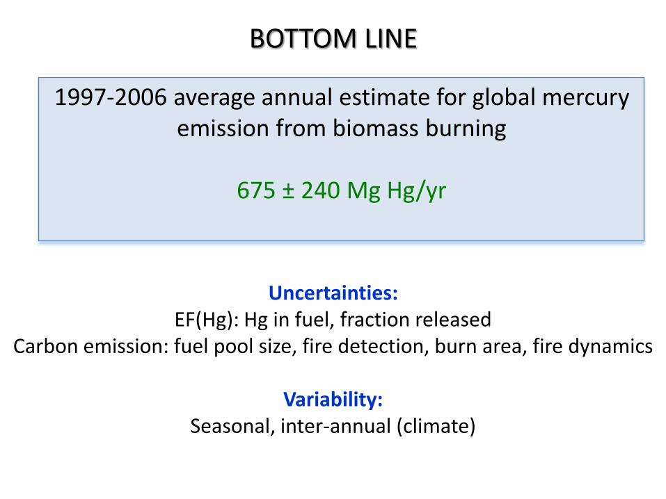
BOTTOM LINE

1997-2006 average annual estimate for global mercury emission from biomass burning

675 ± 240 Mg Hg/yr

Uncertainties:EF(Hg): Hg in fuel, fraction released

Carbon emission: fuel pool size, fire detection, burn area, fire dynamics

Variability:Seasonal, inter-annual (climate)

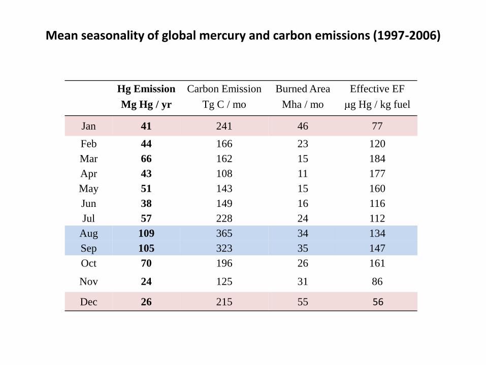
Hg Emission Carbon Emission Burned Area Effective EF

Mg Hg / yr Tg C / mo Mha / mo g Hg / kg fuel

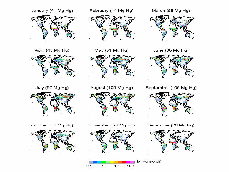
Jan 41 241 46 77

Feb 44 166 23 120

Mar 66 162 15 184

Apr 43 108 11 177

May 51 143 15 160

Jun 38 149 16 116

Jul 57 228 24 112

Aug 109 365 34 134

Sep 105 323 35 147

Oct 70 196 26 161

Nov 24 125 31 86

Dec 26 215 55 56

Mean seasonality of global mercury and carbon emissions (1997-2006)

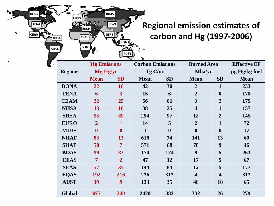
Hg Emissions Carbon Emissions Burned Area Effective EF

Regions Mg Hg/yr Tg C/yr Mha/yr g Hg/kg fuel

Mean SD Mean SD Mean SD Mean

BONA 22 16 42 30 2 1 233

TENA 6 3 16 6 2 0 178

CEAM 22 25 56 61 3 2 175

NHSA 13 10 38 25 4 1 157

SHSA 95 39 294 97 12 2 145

EURO 2 1 14 5 2 1 72

MIDE 0 0 1 0 0 0 17

NHAF 83 13 618 74 141 13 60

SHAF 58 7 571 68 78 9 46

BOAS 99 83 170 124 9 5 263

CEAS 7 2 47 12 17 5 67

SEAS 57 35 144 84 12 5 177

EQAS 192 216 276 312 4 4 312

AUST 19 9 133 35 46 18 65

Global 675 240 2420 382 332 26 279

Regional emission estimates of carbon and Hg (1997-2006)

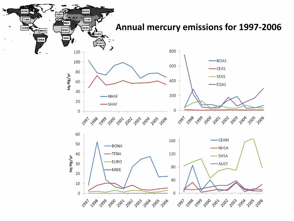
Annual mercury emissions for 1997-2006

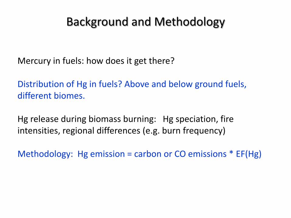
Background and Methodology

Mercury in fuels: how does it get there?

Distribution of Hg in fuels? Above and below ground fuels, different biomes.

Hg release during biomass burning: Hg speciation, fire intensities, regional differences (e.g. burn frequency)

Methodology: Hg emission = carbon or CO emissions * EF(Hg)

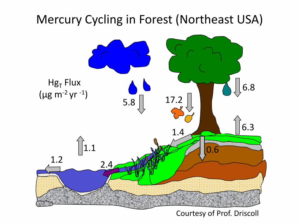
Mercury Cycling in Forest (Northeast USA)

6.8

17.25.8

0.61.1

2.41.2

HgT Flux(µg m-2 yr -1)

1.4 6.3

1.2 2.4

Courtesy of Prof. Driscoll

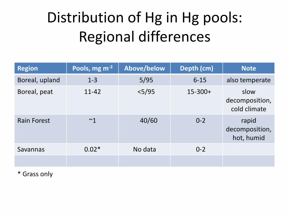
Distribution of Hg in Hg pools: Regional differences

Region Pools, mg m-2 Above/below Depth (cm) Note

Boreal, upland 1-3 5/95 6-15 also temperate

Boreal, peat 11-42 <5/95 15-300+ slow decomposition,

cold climate

Rain Forest ~1 40/60 0-2 rapid decomposition,

hot, humid

Savannas 0.02* No data 0-2

* Grass only

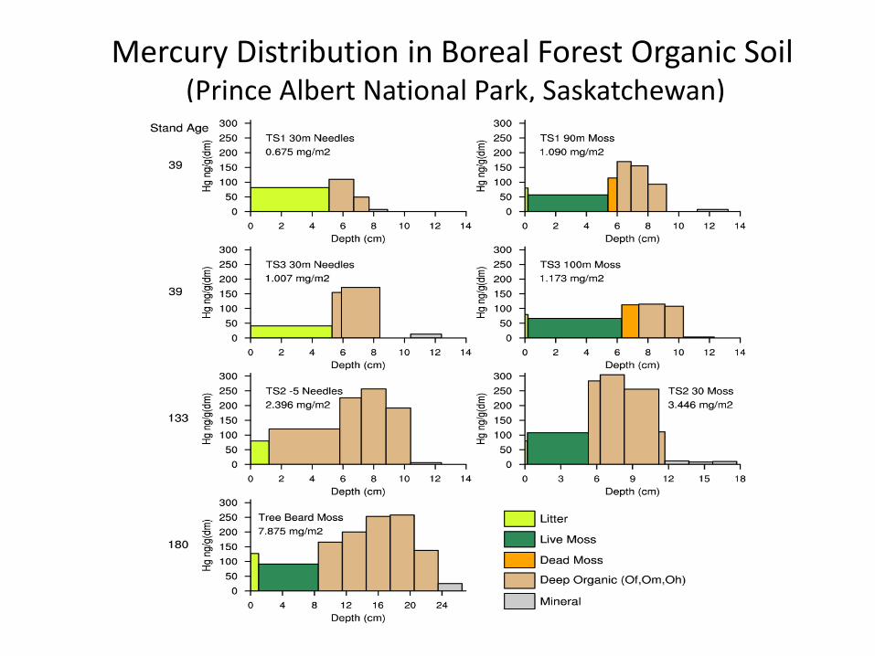
Mercury Distribution in Boreal Forest Organic Soil(Prince Albert National Park, Saskatchewan)

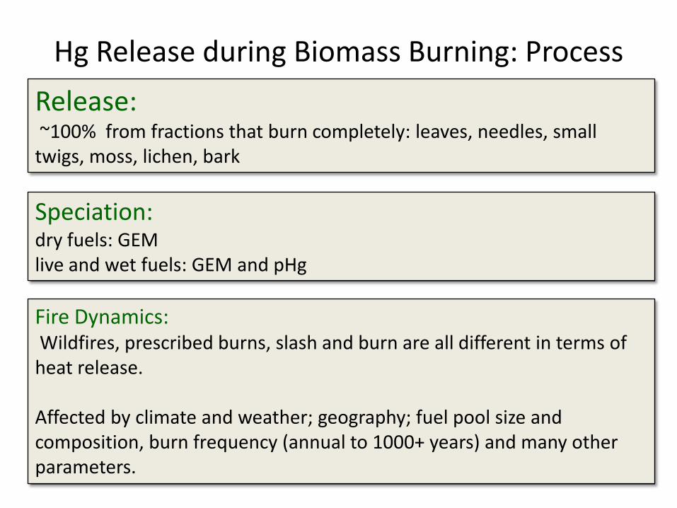
Hg Release during Biomass Burning: Process

Release:~100% from fractions that burn completely: leaves, needles, small twigs, moss, lichen, bark

Speciation: dry fuels: GEM live and wet fuels: GEM and pHg

Fire Dynamics:Wildfires, prescribed burns, slash and burn are all different in terms of heat release.

Affected by climate and weather; geography; fuel pool size and composition, burn frequency (annual to 1000+ years) and many other parameters.

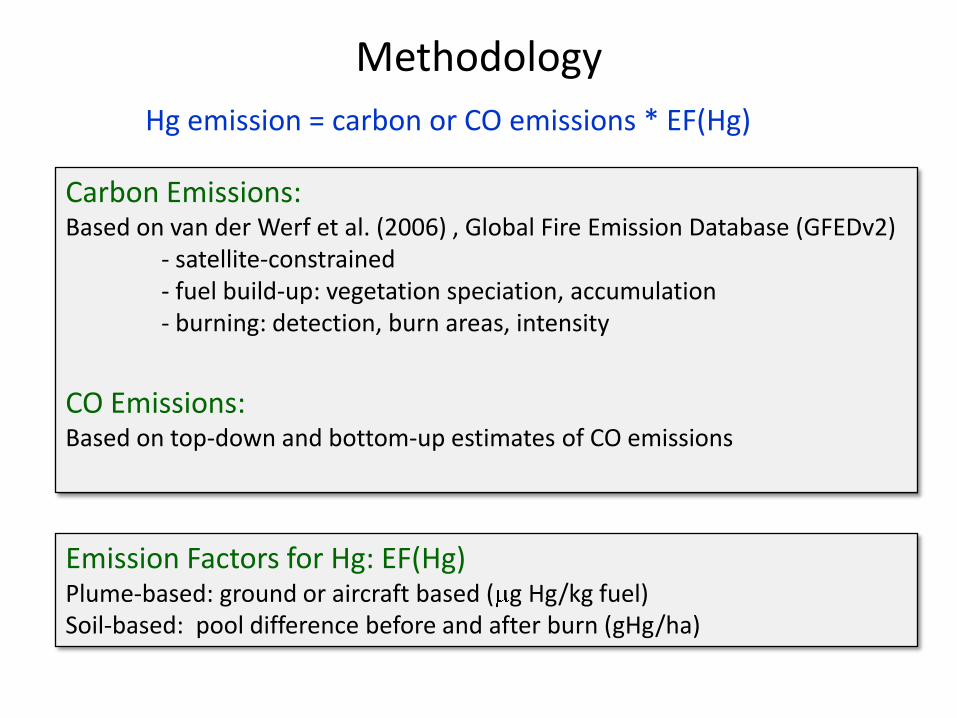
Methodology

Hg emission = carbon or CO emissions * EF(Hg)

Carbon Emissions:Based on van der Werf et al. (2006) , Global Fire Emission Database (GFEDv2)

- satellite-constrained- fuel build-up: vegetation speciation, accumulation- burning: detection, burn areas, intensity

CO Emissions:Based on top-down and bottom-up estimates of CO emissions

Emission Factors for Hg: EF(Hg)Plume-based: ground or aircraft based ( g Hg/kg fuel)Soil-based: pool difference before and after burn (gHg/ha)

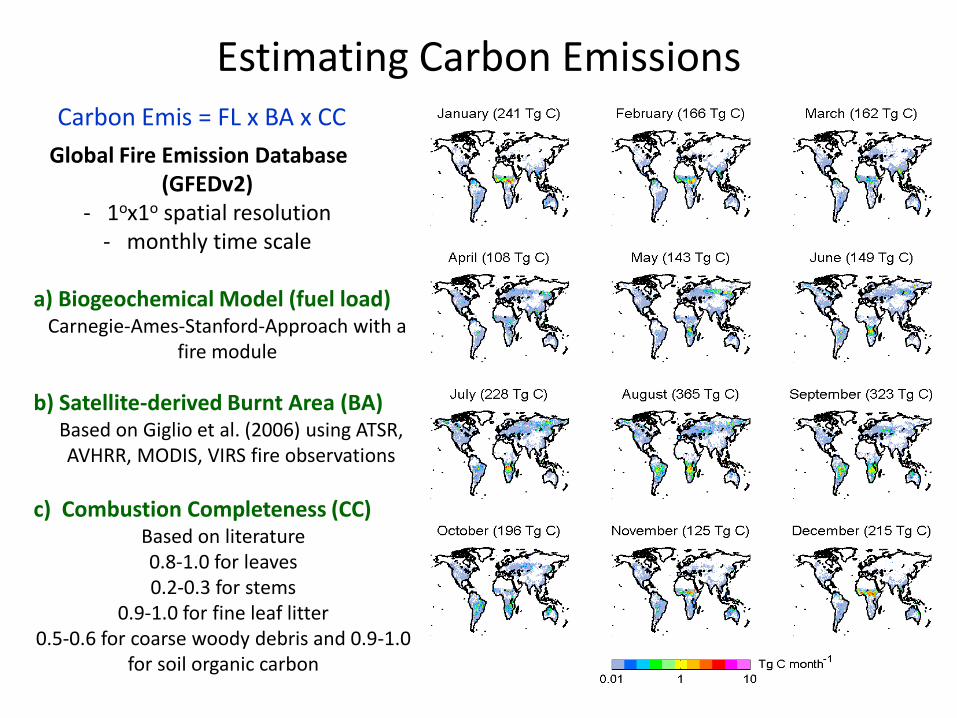
Estimating Carbon Emissions

Global Fire Emission Database(GFEDv2)

- 1ox1o spatial resolution- monthly time scale

a) Biogeochemical Model (fuel load)Carnegie-Ames-Stanford-Approach with a

fire module

b) Satellite-derived Burnt Area (BA)Based on Giglio et al. (2006) using ATSR, AVHRR, MODIS, VIRS fire observations

c) Combustion Completeness (CC)Based on literature 0.8-1.0 for leaves0.2-0.3 for stems

0.9-1.0 for fine leaf litter0.5-0.6 for coarse woody debris and 0.9-1.0

for soil organic carbon

Carbon Emis = FL x BA x CC

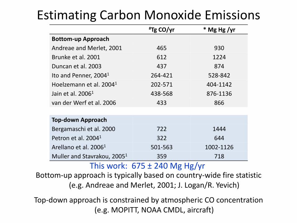
Estimating Carbon Monoxide Emissions#Tg CO/yr * Mg Hg /yr

Bottom-up Approach

Andreae and Merlet, 2001 465 930

Brunke et al. 2001 612 1224

Duncan et al. 2003 437 874

Ito and Penner, 20041 264-421 528-842

Hoelzemann et al. 20041 202-571 404-1142

Jain et al. 20061 438-568 876-1136

van der Werf et al. 2006 433 866

Top-down Approach

Bergamaschi et al. 2000 722 1444

Petron et al. 20041 322 644

Arellano et al. 20061 501-563 1002-1126

Muller and Stavrakou, 20051 359 718

This work: 675 ± 240 Mg Hg/yrBottom-up approach is typically based on country-wide fire statistic

(e.g. Andreae and Merlet, 2001; J. Logan/R. Yevich)

Top-down approach is constrained by atmospheric CO concentration(e.g. MOPITT, NOAA CMDL, aircraft)

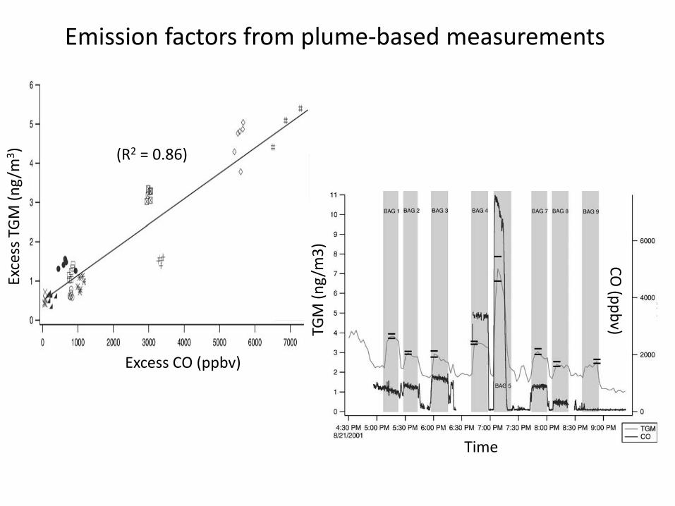
Emission factors from plume-based measurements

Time

Exce

ss T

GM

(n

g/m

3)

TGM

(n

g/m

3)

Excess CO (ppbv)

CO

(pp

bv)

(R2 = 0.86)

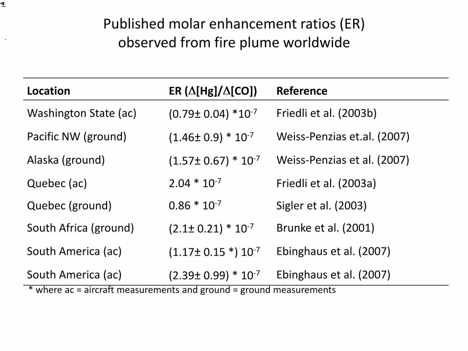
Location ER ( [Hg]/ [CO]) Reference

Washington State (ac) (0.79± 0.04) *10-7 Friedli et al. (2003b)

Pacific NW (ground) (1.46± 0.9) * 10-7 Weiss-Penzias et.al. (2007)

Alaska (ground) (1.57± 0.67) * 10-7 Weiss-Penzias et al. (2007)

Quebec (ac) 2.04 * 10-7 Friedli et al. (2003a)

Quebec (ground) 0.86 * 10-7 Sigler et al. (2003)

South Africa (ground) (2.1± 0.21) * 10-7 Brunke et al. (2001)

South America (ac) (1.17± 0.15 *) 10-7 Ebinghaus et al. (2007)

South America (ac) (2.39± 0.99) * 10-7 Ebinghaus et al. (2007)

.

Published molar enhancement ratios (ER) observed from fire plume worldwide

* where ac = aircraft measurements and ground = ground measurements

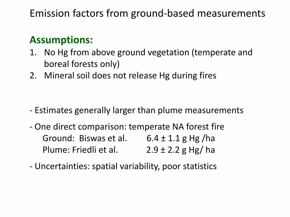
Emission factors from ground-based measurements

Assumptions: 1. No Hg from above ground vegetation (temperate and

boreal forests only)2. Mineral soil does not release Hg during fires

- Estimates generally larger than plume measurements

- One direct comparison: temperate NA forest fireGround: Biswas et al. 6.4 ± 1.1 g Hg /haPlume: Friedli et al. 2.9 ± 2.2 g Hg/ ha

- Uncertainties: spatial variability, poor statistics

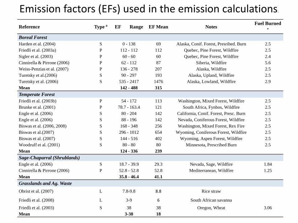
Emission factors (EFs) used in the emission calculations.

Reference Type # EF Range EF Mean NotesFuel Burned

*

Boreal Forest

Harden et al. (2004) S 0 - 138 69 Alaska, Conif. Forest, Presribed. Burn 2.5

Friedli et al. (2003a) P 112 - 112 112 Quebec, Pine Forest, Wildfire 2.5

Sigler et al. (2003) P 60 - 60 60 Quebec, Pine Forest, Wildfire 2.4

Cinnirella & Pirrone (2006) P 62 - 112 87 Siberia, Wildfire 5.6

Weiss-Penzias et al. (2007) P 136 - 278 207 Alaska, Wildfire 2.5

Turetsky et al.(2006) S 90 - 297 193 Alaska, Upland, Wildfire 2.5

Turetsky et al. (2006) S 535 - 2417 1476 Alaska, Lowland, Wildfire 2.9

Mean 142 - 488 315

Temperate Forest

Friedli et al. (2003b) P 54 - 172 113 Washington, Mixed Forest, Wildfire 2.5

Brunke et al. (2001) P 78.7 - 163.4 121 South Africa, Fynbos, Wildfire 2.5

Engle et al. (2006) S 80 - 204 142 California, Conif. Forest, Presc. Burn 2.5

Engle et al. (2006) S 88 - 196 142 Nevada, Coniferous Forest, Wildfire 2.5

Biswas et al. (2006, 2008) S 168 - 348 256 Washington, Mixed Forest, Rex Fire 2.5

Biswas et al.(2007) S 296 - 1012 654 Wyoming, Coniferous Forest, Wildfire 2.5

Biswas et al. (2007) S 144 - 516 402 Wyoming, Aspen Forest, Wildfire 2.5

Woodruff et al. (2001) S 80 - 80 80 Minnesota, Prescribed Burn 2.5

Mean 124 - 336 239

Sage-Chaparral (Shrublands)

Engle et al. (2006) S 18.7 - 39.9 29.3 Nevada, Sage, Wildfire 1.84

Cinnirella & Pirrone (2006) P 52.8 - 52.8 52.8 Mediterranean, Wildfire 1.25

Mean 35.8 - 46.4 41.1

Grasslands and Ag. Waste

Obrist et al. (2007) L 7.8-9.8 8.8 Rice straw

Friedli et al. (2008) L 3-9 6 South African savanna

Friedli et al. (2003) S 38 38 Oregon, Wheat 3.06

Mean 3-38 18

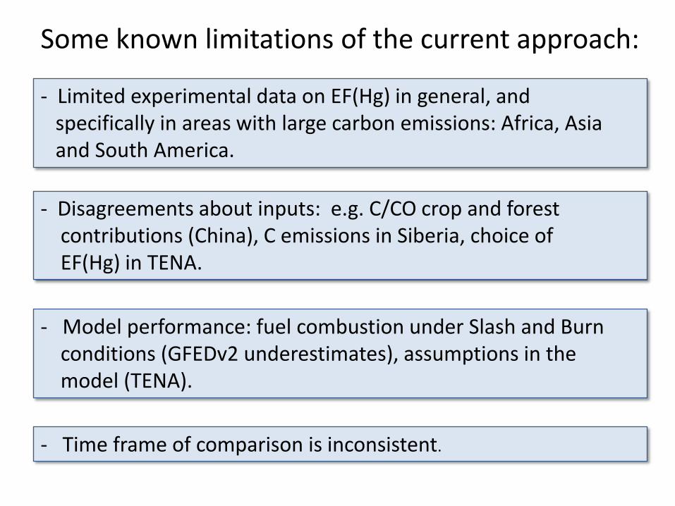
Some known limitations of the current approach:

- Limited experimental data on EF(Hg) in general, and specifically in areas with large carbon emissions: Africa, Asia and South America.

- Disagreements about inputs: e.g. C/CO crop and forest contributions (China), C emissions in Siberia, choice of EF(Hg) in TENA.

- Model performance: fuel combustion under Slash and Burn conditions (GFEDv2 underestimates), assumptions in the model (TENA).

- Time frame of comparison is inconsistent.

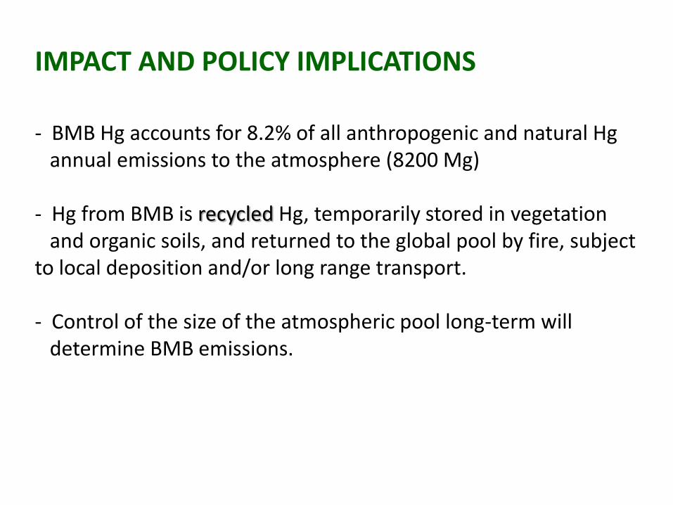
IMPACT AND POLICY IMPLICATIONS

- BMB Hg accounts for 8.2% of all anthropogenic and natural Hg annual emissions to the atmosphere (8200 Mg)

- Hg from BMB is recycled Hg, temporarily stored in vegetation and organic soils, and returned to the global pool by fire, subject

to local deposition and/or long range transport.

- Control of the size of the atmospheric pool long-term will determine BMB emissions.

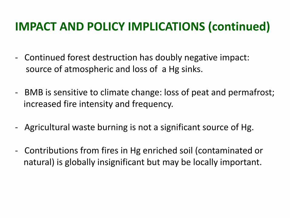
IMPACT AND POLICY IMPLICATIONS (continued)

- Continued forest destruction has doubly negative impact:source of atmospheric and loss of a Hg sinks.

- BMB is sensitive to climate change: loss of peat and permafrost; increased fire intensity and frequency.

- Agricultural waste burning is not a significant source of Hg.

- Contributions from fires in Hg enriched soil (contaminated or natural) is globally insignificant but may be locally important.

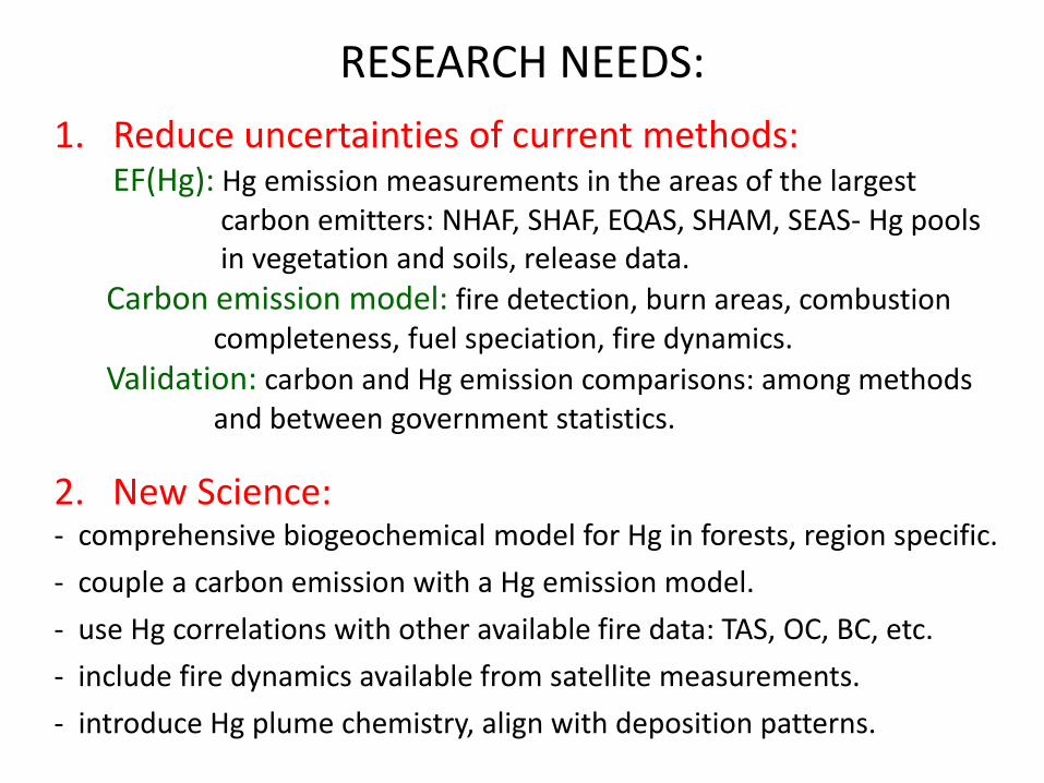
RESEARCH NEEDS:

1. Reduce uncertainties of current methods:EF(Hg): Hg emission measurements in the areas of the largest

carbon emitters: NHAF, SHAF, EQAS, SHAM, SEAS- Hg pools in vegetation and soils, release data.

Carbon emission model: fire detection, burn areas, combustion completeness, fuel speciation, fire dynamics.

Validation: carbon and Hg emission comparisons: among methods and between government statistics.

2. New Science:- comprehensive biogeochemical model for Hg in forests, region specific.

- couple a carbon emission with a Hg emission model.

- use Hg correlations with other available fire data: TAS, OC, BC, etc.

- include fire dynamics available from satellite measurements.

- introduce Hg plume chemistry, align with deposition patterns.

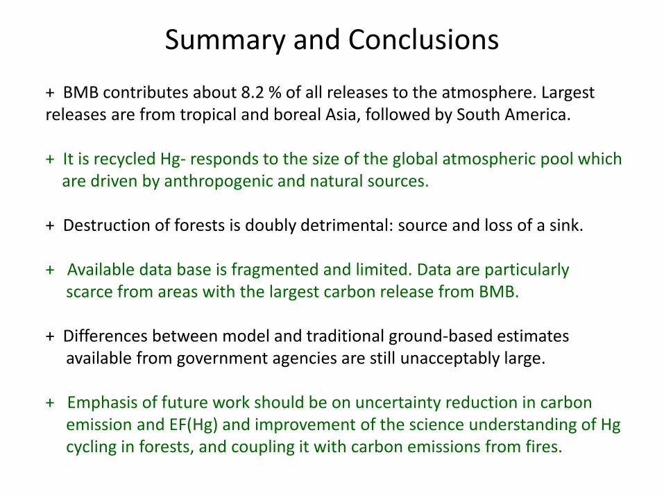
Summary and Conclusions

+ BMB contributes about 8.2 % of all releases to the atmosphere. Largest releases are from tropical and boreal Asia, followed by South America.

+ It is recycled Hg- responds to the size of the global atmospheric pool which are driven by anthropogenic and natural sources.

+ Destruction of forests is doubly detrimental: source and loss of a sink.

+ Available data base is fragmented and limited. Data are particularly scarce from areas with the largest carbon release from BMB.

+ Differences between model and traditional ground-based estimatesavailable from government agencies are still unacceptably large.

+ Emphasis of future work should be on uncertainty reduction in carbon emission and EF(Hg) and improvement of the science understanding of Hg cycling in forests, and coupling it with carbon emissions from fires.

Acknowledgements

- James T. Randerson (PI) of University of California, Irvine, Guido R. van derWerf of Vrije Universiteit Amsterdam, Louis Giglio of Science Systems and Applications, Inc., Maryland, G. James Collatz of NASA Goddard Space Flight Center, Maryland and Prasad S. Kasibhatla of Duke University for GFEDv2 emission data.

- support from the National Center for Atmospheric Research, which sponsored by the National Science Foundation.