Semiconductor Optoelectronics (Farhan Rana, Cornell University)

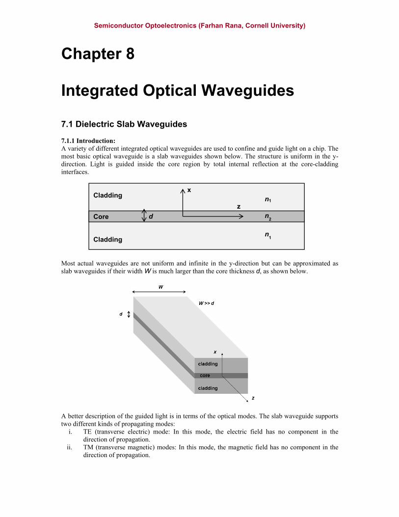
Chapter 8 Integrated Optical Waveguides 7.1 Dielectric Slab Waveguides 7.1.1 Introduction: A variety of different integrated optical waveguides are used to confine and guide light on a chip. The most basic optical waveguide is a slab waveguides shown below. The structure is uniform in the y-direction. Light is guided inside the core region by total internal reflection at the core-cladding interfaces.

Most actual waveguides are not uniform and infinite in the y-direction but can be approximated as slab waveguides if their width W is much larger than the core thickness d, as shown below.

A better description of the guided light is in terms of the optical modes. The slab waveguide supports two different kinds of propagating modes:

i. TE (transverse electric) mode: In this mode, the electric field has no component in the direction of propagation.

ii. TM (transverse magnetic) modes: In this mode, the magnetic field has no component in the direction of propagation.

Cladding

Cladding

Core

z

xn1

n2

n1

d

Semiconductor Optoelectronics (Farhan Rana, Cornell University)

To study these modes we start from Maxwell’s equations. The complex form of Maxwell’s equations is,

Exnc

E

ExniH

HiE

o

o

)(

)(

22

2

2

Since EEE

2)( . In general 0 E

. Rather 0])([ 2 Exn

. But if index

is piecewise uniform in different regions then inside each region one may assume 0 E

. So we have in each region,

Exnc

E

)(22

22

Similarly, with the assumption of piecewise uniform index we can write for theH

field,

Hxnc

H

)(22

22

7.1.2 TE Modes: For TE modes, the electric field can be written as,

zio exEyzxE )(ˆ),(

In each region of piecewise uniform index (core and cladding), )(x satisfies,

)()()( 222

2

2

2xxxn

cx

Given a value for the frequency , we can find all solutions of the above equation which is an

eigenvalue equation with eigenfunction )(x and eigenvalue 2 . Once we have the electric field,

the magnetic field H

can be found as follows,

zi

o

o

o

o

o

exE

xx

x

i

Ez

i

zxEzix

x

i

EzxH

)(ˆ)(ˆ

),(ˆˆ

),(0

The boundary conditions needed to solve the eigenvalue equation above are as follows:

i) y-component of the electric field is continuous at the core-cladding interfaces ii) z-component of the magnetic field is continuous at the core-cladding interfaces iii) x-component of the magnetic field is continuous at the core-cladding interfaces (this is

automatically satisfied when (i) above is satisfied) The solutions are labeled with the integer index ).,3,2,1,0( mm So the field for the TEm mode is,

zimo

mexEyzxE )(),(ˆ),(

where the dependence of the eigenfunctions and the propagation vector on the frequency is

explicitly indicated. For the TE modes we assume the solution,

2/

2/||)sin(

)cos(2/

)(

)2/(1

2

)2/(1

dxeC

dxkx

kxC

dxeC

x

dx

dx

Semiconductor Optoelectronics (Farhan Rana, Cornell University)

Plugging the above solutions in the equation,

)()()( 222

2

2

2xxxn

cx

we get,

221

222

2

212

222

222

222

)( knnc

nc

nc

k

Using the boundary conditions give,

)modesTEoddsolutionssine(2

cot

)modesTEevensolutionscosine(2

tan

k

kd

k

kd

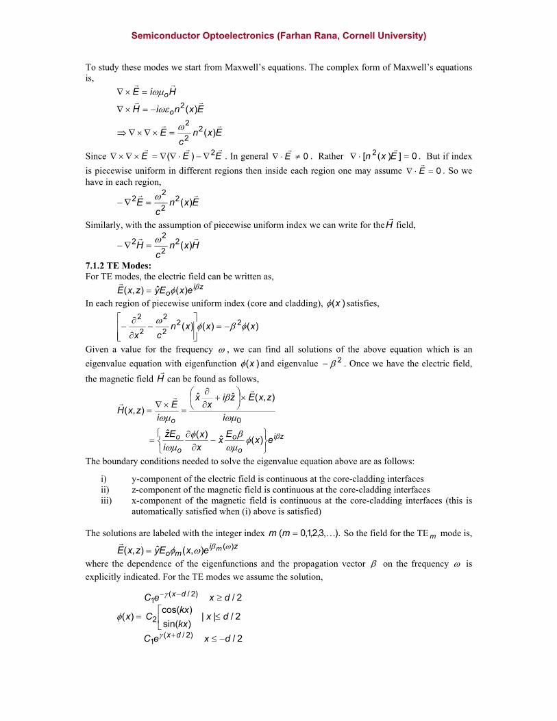
A solution can be obtained graphically by plotting the left and right sides of the above equations, as shown below where the left side is plotted using blue lines and right side using red lines. Below a certain frequency m the m-the mode ceases to exist. This cut-off frequency is,

21

22 nn

c

dmm

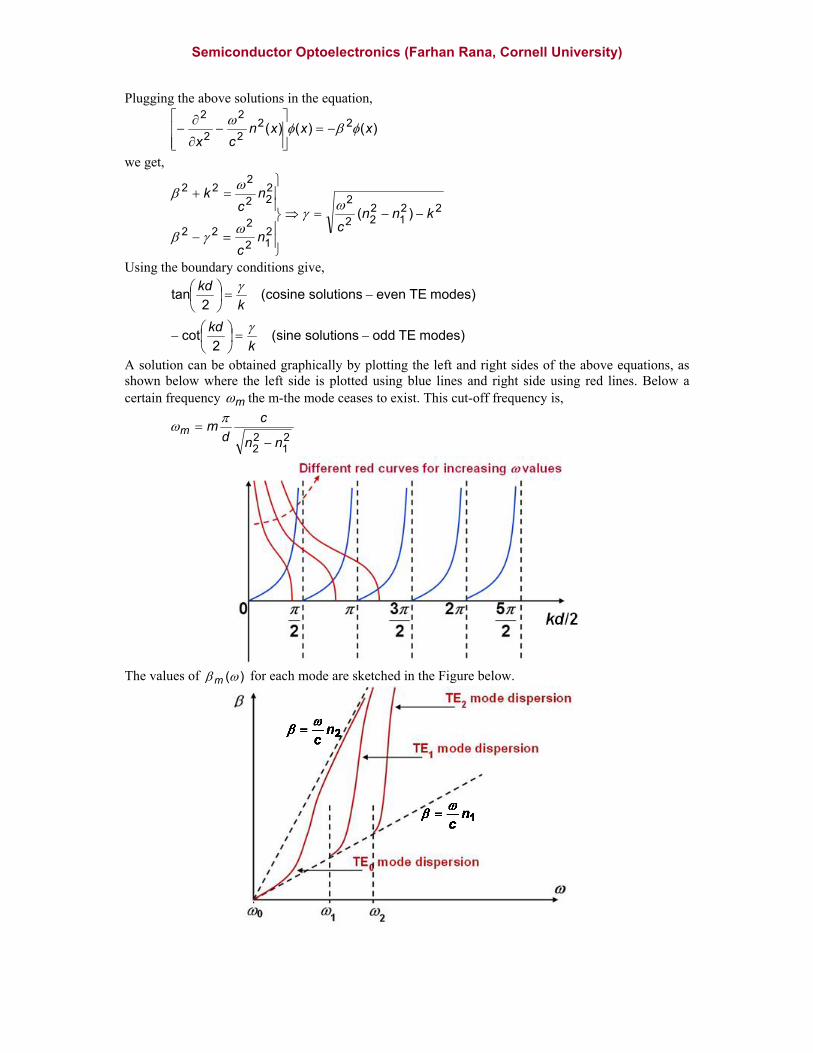
The values of )(m for each mode are sketched in the Figure below.

Semiconductor Optoelectronics (Farhan Rana, Cornell University)

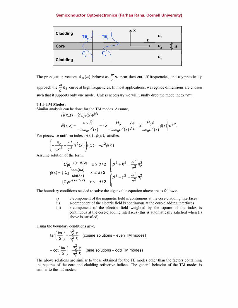
The propagation vectors )(m behave as 1nc

near then cut-off frequencies, and asymptotically

approach the 2nc

curve at high frequencies. In most applications, waveguide dimensions are chosen

such that it supports only one mode. Unless necessary we will usually drop the mode index “m“. 7.1.3 TM Modes: Similar analysis can be done for the TM modes. Assume,

.)()(

ˆ)(

ˆ)(

),(

)(ˆ),(

222zi

o

o

o

o

o

zio

exxn

Hx

xxni

Hz

xni

HzxE

exHyzxH

For piecewise uniform index )(xn , ),(x satisfies,

)()()( 222

2

22 xxxn

cx

Assume solution of the form,

212

222

222

222

)2/(1

2

)2/(1

2/

2/||)sin(

)cos(2/

)(n

c

nc

k

dxeC

dxkx

kxC

dxeC

x

dx

dx

The boundary conditions needed to solve the eigenvalue equation above are as follows:

i) y-component of the magnetic field is continuous at the core-cladding interfaces ii) z-component of the electric field is continuous at the core-cladding interfaces iii) x-component of the electric field weighted by the square of the index is

continuous at the core-cladding interfaces (this is automatically satisfied when (i) above is satisfied)

Using the boundary conditions give,

)modesTModdsolutionssine(2

cot

)modesTMevensolutionscosine(2

tan

21

22

21

22

kn

nkd

kn

nkd

The above relations are similar to those obtained for the TE modes other than the factors containing the squares of the core and cladding refractive indices. The general behavior of the TM modes is similar to the TE modes.

Cladding

Cladding

Core

z

xn1

n2

n1

d

Ey E

y

TE0 TE

1

Semiconductor Optoelectronics (Farhan Rana, Cornell University)

7.1.4 Effective Index and Group Index: The effective index )(effn of a mode is defined by the relation,

)()( effnc

The effective index of each mode equals 1n at their cut-off frequencies and approaches 2n at high

frequencies. The group velocity of a mode is,

)(

1

gv

gv is written as,

)(

)(

g

g n

cv

where )(gn is called the group index of the mode.

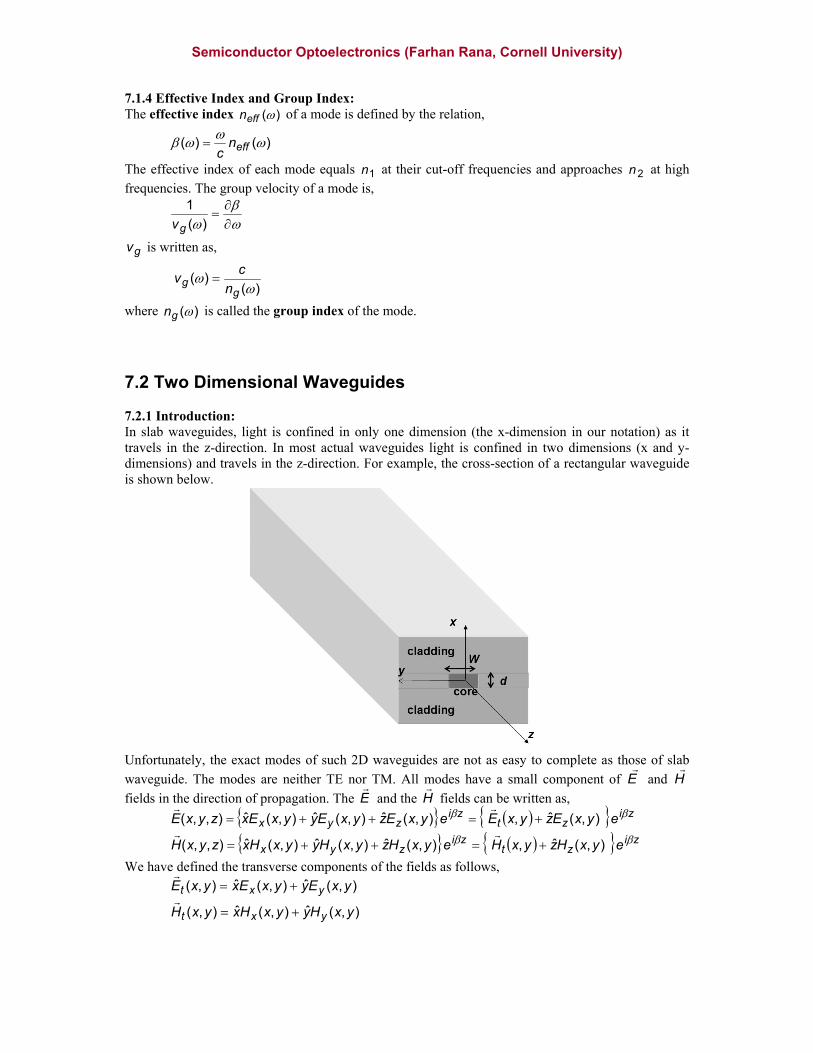
7.2 Two Dimensional Waveguides 7.2.1 Introduction: In slab waveguides, light is confined in only one dimension (the x-dimension in our notation) as it travels in the z-direction. In most actual waveguides light is confined in two dimensions (x and y- dimensions) and travels in the z-direction. For example, the cross-section of a rectangular waveguide is shown below.

Unfortunately, the exact modes of such 2D waveguides are not as easy to complete as those of slab

waveguide. The modes are neither TE nor TM. All modes have a small component of E

and H

fields in the direction of propagation. The E

and the H

fields can be written as,

zizt

zizyx eyxEzyxEeyxEzyxEyyxExzyxE ),(ˆ,),(ˆ),(ˆ),(ˆ),,(

zizt

zizyx eyxHzyxHeyxHzyxHyyxHxzyxH ),(ˆ,),(ˆ),(ˆ),(ˆ),,(

We have defined the transverse components of the fields as follows,

),(ˆ),(ˆ),(

),(ˆ),(ˆ),(

yxHyyxHxyxH

yxEyyxExyxE

yxt

yxt

Semiconductor Optoelectronics (Farhan Rana, Cornell University)

Since the exact solution is difficult and cumbersome, several levels of approximations are commonly used and are discussed below. 7.2.2 Mode Solutions for 2D Waveguides: We need to solve the equation,

oi

EHyxEyxn

czyxE

),(),(),,( 22

2

subject to all the proper boundary conditions for the E

and H

fields at all the interfaces. The operator is,

z

zy

yx

x

ˆˆˆ

Define,

z

zy

yx

x tt

ˆˆˆ

From HiE o

, it follows that,

)1(ˆ).(

ˆ).(

ˆ.ˆ).(

o

ttz

zott

zizoo

i

zEH

HizE

eHizHizE

Similarly it can be shown that,

)2(ˆ).(

2ni

zHE

o

ttz

Equations (1) and (2) show that knowing the transverse components of the field is enough since the z-components can be determined from the transverse components. We need to solve,

Eyxnc

EE

Eyxnc

E

),(.

),(

22

22

22

2

Taking the transverse component gives,

)3(0).( 22

22 zi

tzi

tt eEnc

eEE

We need to find convenient and useful expressions for the first two terms on the right hand side. Now,

ziz

zitt eEieEE

.. but,

zittt

zitttt

zittzitt

ziz

zitt

ttz

ztt

en

EneEE

en

EneEeEieEE

n

EnEi

EniEn

En

2

2

2

2

2

2

22

2

).(.).(

).(...

).(

0).(

0).(

The other term in Equation (3) is,

Semiconductor Optoelectronics (Farhan Rana, Cornell University)

zit

zitt

zit eEeEeE

222

Using the results above, Equation (3) becomes,

ttttttttt EEnc

Enn

EE

222

22

22 ).(

1.

The above eigenvalue equation is what one needs to solve to get the exact solution. This equation can be put in the form,

)4(ˆˆ

ˆˆ2

y

x

y

x

yyyx

xyxx

E

E

E

E

PP

PP

where the differential operators are.

yx

E

y

En

nxEP

Ency

E

x

En

nxEP

yyyxy

xxx

xxx

22

2

22

2

2

22

2

)(1ˆ

)(1ˆ

xy

E

x

En

nyEP

Ency

En

nyx

EEP

xxxyx

yyy

yyy

22

2

22

22

22

2

)(1ˆ

)(1ˆ

The above equation is an eigenvalue equation and its solution gives the transverse components of the

electric field E

for the mode and the corresponding propagation constant )( . ),( yxEz can be

obtained from ),( yxE x and ),( yxE y as already explained, and H

field can be obtained from the

relation,

0

)(

iE

H

For piecewise uniform indices, all derivatives of the index ),( yxn can be dropped provided appropriate boundary conditions are used at all the interfaces. 7.2.3 The Semi-Vectorial Approximation: In many cases of practical interest one transverse component of the electric field (either xE or yE )

dominates over the other component. In such cases, we may assume that the other transverse field component is zero. For example, if we know a priori that xE dominates then we may assume that

yE is zero and solve the much simpler eigenvalue equation,

.)),()(1

ˆ

222

2

2

22

2

2

xxxx

xxxx

EEyxncy

E

x

En

nx

EEP

The above equation is called the semi-vectorial approximation. For piecewise uniform dielectrics we can also write it as,

xxxt

xxxx

EEyxnc

E

EEyxnc

Ey

Ex

222

22

222

2

2

2

2

2

),(

),(

Semiconductor Optoelectronics (Farhan Rana, Cornell University)

provided we take care to impose the boundary conditions on ),( yxEx at all the dielectric interfaces

as appropriate for the x-component of the electric field. Once the dominant ),( yxEx component has been found, the remaining field components can be found as follows,

y

E

iH

H

x

En

nyH

x

En

nxEH

i

EH

x

En

n

iE

En

x

oz

x

ox

x

ox

oy

o

xz

1

0.

11

11

)(

1

0.

2

2

2

2

2

2

2

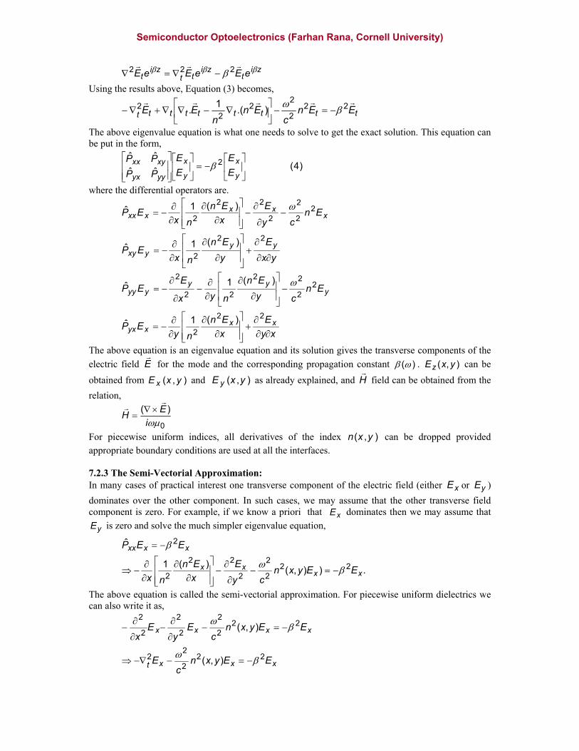
When the horizontal electric field component dominates the modes are sometimes called HEpq modes or TEpq modes (with a slight abuse of terminology). When the vertical electric field component dominates the modes are called EHpq modes or TMpq modes (again with a slight abuse of terminology). The two subscripts p and q indicate the number of nodes the dominant electric field component has in the horizontal and vertical directions, respectively.

7.2.4 The Scalar Field Approximation: If one component of the transverse electric field dominates over the other transverse component and the index differences among different regions in the structure are also relatively small, then one may use the semi-vectorial approximation and also do away with the boundary conditions on the normal component of the electric field at all dielectric interfaces. For example, if we know a priori that

),( yxEx dominates then we may solve the equation,

Semiconductor Optoelectronics (Farhan Rana, Cornell University)

),(),(),(),(

),(),(),(),(),(

222

22

222

2

2

2

2

2

yxEyxEyxnc

yxE

yxEyxEyxnc

yxEy

yxEx

xxxt

xxxx

assuming that the field and its derivative are continuous across all dielectric interfaces. This is called the scalar field approximation. Once the dominant electric field component has been found, the remaining field components can be found as in the case of the semi-vectorial approximation. Scalar field approximation seems crude but it gives very accurate answers for the propagation vector )(

(or the effective index )(effn ) as long as one is for away from the mode cut-off frequency. It is also very accurate in calculating mode confinement factors – as we will see in later Chapters. For most part of this course we will use the scalar field approximation to keep the computational overhead low. One disadvantage of the scalar field approximation is that it does not tell accurately whether the single-mode condition holds since the scalar field approximation is not accurate near mode cut-off. 7.2.5 Slab Waveguide Approximation: If the aspect ratio of the waveguide is such that one dimension is much larger than the other dimension, then the modes and the corresponding wavevectors and effective indices can be approximated by those of the corresponding slab waveguide as discussed earlier. 7.2.6 Energy and Power in Waveguides: The energy flow for electromagnetic fields is given by the complex Poynting vector,

)]()(*)(*)([4

1)(

)](*)(Re[2

1)(

rHrErHrErS

rHrErS

For waveguides electric and magnetic fields are of the form,

zi

zyx

zizyx

eyxHzyxHyyxHxzyxH

eyxEzyxEyyxExzyxE

),(ˆ),(ˆ),(ˆ),,(

),(ˆ),(ˆ),(ˆ),,(

The total energy flow (or power) in a waveguide is obtained by integrating the Poynting vector over the cross-section of the waveguide,

dxdyzHEHEdxdyzHEHEdxdyzSzP tttt ˆ.]**[4

1ˆ.]**[4

1ˆ.)(

Assuming the medium to be dispersive, the energy per unit length of the waveguide is,

dxdyHHEEnnn

dxdyHHEEzW

oMgo

oo

*.4

1*.2

4

1

*.4

1*.

4

1

Here, Mgn is the material group index, defined earlier as,

d

dnnnMg

The superscript “M“ is intended so as not to cause confusion with the group index of the optical mode. The following relation can also be proven,

dxdyHHdxdyEEn oo *.4

1*.

4

1 2

Therefore, the energy per unit length can be written as,

Semiconductor Optoelectronics (Farhan Rana, Cornell University)

dxdyEEnnzW Mgo *.

2

1

The effective index )(effn of a mode is,

)()( effnc

The group velocity of a mode is,

)(

1

gv

gv is frequently expressed in terms of the group index of the mode,

)(

)(

g

g n

cv

where )(gn is called the group index. One can prove the following relation between the power

)(zP and the energy per unit length )(zW ,

)()( zWvzP g

which can also be written as,

dxdyzHE

dxdyEEnn

zP

zW

c

n

tt

Mgog

ˆ.*Re

*.

)(

)(

In the slab-waveguide approximation, assuming TE modes with the transverse component of the electric field given by yx, , one obtains the following expressions for various quantities of interest,

dxdynndxdyEEnnzW Mgo

Mgo

2

2

1*.

2

1

dxdydxdyzHEHEzPo

tttt 2

2

1ˆ.]**[4

1)(

dxdy

dxdynnnn

Mg

effg 2

2

7.2.7 Properties of Waveguide Modes and Orthogonality of Modes: Frequently, solutions in various cases involve expansions in terms of all the waveguide modes. In such cases, knowledge of the orthogonality of the modes is useful. The electric and the magnetic fields for the m-th mode can be written as,

zimz

mt

m meyxEzyxEE ),(ˆ,

zimz

mt

m meyxHzyxHH ),(ˆ,

Some useful properties of the waveguides modes are listed below: i) When the indices are real, the propagation vectors are also real, and the transverse field components can be chosen to be real as well. Equations (1) and (2) show that in this case the z-components of the fields are purely imaginary. ii) When the indices are real, the complex conjugate of the electric field mode gives the field for the mode propagating in the opposite (time-reversed) direction. For example, if,

zimz

mt

m meyxEzyxEE ),(ˆ,

represents the field for the forward propagating mode then,

zimz

mt

m meyxEzyxEE ),(ˆ,*

represents the field for the backward propagating mode.

Semiconductor Optoelectronics (Farhan Rana, Cornell University)

iii) When the indices are real, the negative of the complex conjugate of the magnetic field mode gives the field for the mode propagating in the opposite (time-reversed) direction. For example, if,

zimz

mt

m meyxHzyxHH ),(ˆ,

represents the field for the forward propagating mode then,

zimz

mt

m meyxHzyxHH ),(ˆ,*

represents the field for the backward propagating mode. iv) Consider two different modes, “m“ and “p“ with the same propagation vector but different frequencies then the orthogonality between the mode fields is expressed as,

pmEEyxndxdy pm for0*.,2

pmHHdxdy pm for0*.

v) Consider two different modes, “m“ and “p“ with the same frequency but different propagation vectors then the orthogonality between the mode fields is expressed as,

pmzHEdxdy pt

mt for0ˆ.*

vi) The most general way of expanding a time harmonic field of a particular frequency inside a waveguide is in terms of the waveguide modes,

m

zimz

mtm

m

zimz

mtm

mm eyxEzyxEbeyxEzyxEazyxE ),(ˆ,),(ˆ,,,

m

zimz

mtm

m

zimz

mtm

mm eyxHzyxHbeyxHzyxHazyxH ),(ˆ,),(ˆ,,,

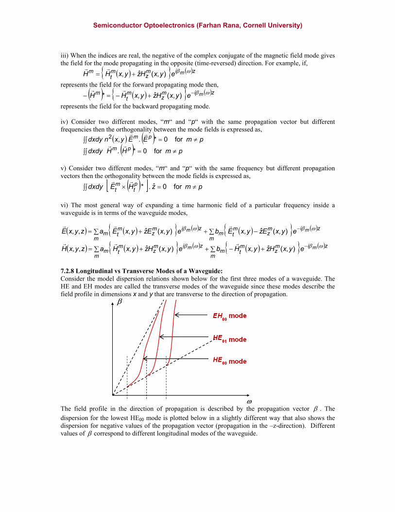
7.2.8 Longitudinal vs Transverse Modes of a Waveguide: Consider the model dispersion relations shown below for the first three modes of a waveguide. The HE and EH modes are called the transverse modes of the waveguide since these modes describe the field profile in dimensions x and y that are transverse to the direction of propagation.

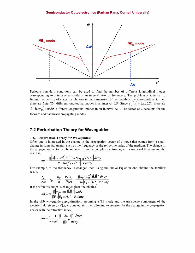
The field profile in the direction of propagation is described by the propagation vector . The

dispersion for the lowest HE00 mode is plotted below in a slightly different way that also shows the dispersion for negative values of the propagation vector (propagation in the –z-direction). Different values of correspond to different longitudinal modes of the waveguide.

HE00 mode

HE01 mode

EH00

mode

Semiconductor Optoelectronics (Farhan Rana, Cornell University)

Periodic boundary conditions can be used to find the number of different longitudinal modes corresponding to a transverse mode in an interval of frequency. The problem is identical to finding the density of states for photons in one dimension. If the length of the waveguide is L then there are 2L different longitudinal modes in an interval . Since gv , there are

22 gvL different longitudinal modes in an interval . The factor of 2 accounts for the

forward and backward propagating modes.

7.2 Perturbation Theory for Waveguides 7.2.7 Perturbation Theory for Waveguides: Often one is interested in the change in the propagation vector of a mode that comes from a small change in some parameter, such as the frequency or the refractive index of the medium. The change in the propagation vector can be obtained from the complex electromagnetic variational theorem and the result is,

dxdyzHE

dxdyHHEEn

tt

o

ˆ.*Re2

*.*. 02

For example, if the frequency is changed then using the above Equation one obtains the familiar result,

dxdyzHE

dxdyEEnn

zP

zW

c

nv

tt

Mgog

gˆ.*Re

*.

)(

)(

If the refractive index is changed then one obtains,

dxdyzHE

dxdyEEnn

tt

o

ˆ.*Re

*.

In the slab waveguide approximation, assuming a TE mode and the transverse component of the electric field given by yx, , one obtains the following expression for the change in the propagation vector with the refractive index,

dxdy

dxdynn

nc eff2

21

HE00

mode HE

00 mode

Semiconductor Optoelectronics (Farhan Rana, Cornell University)

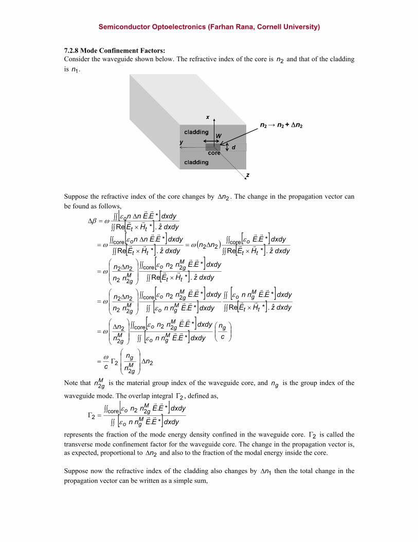
7.2.8 Mode Confinement Factors: Consider the waveguide shown below. The refractive index of the core is 2n and that of the cladding

is 1n .

Suppose the refractive index of the core changes by 2n . The change in the propagation vector can be found as follows,

22

2

core 22

2

2

core 22

22

22

core 22

22

22

core22

core

*.

*.

ˆ.*Re

*.

*.

*.

ˆ.*Re

*.

ˆ.*Re

*.

ˆ.*Re

*.

ˆ.*Re

*.

nn

n

c

c

n

dxdyEEnn

dxdyEEnn

n

n

dxdyzHE

dxdyEEnn

dxdyEEnn

dxdyEEnn

nn

nn

dxdyzHE

dxdyEEnn

nn

nn

dxdyzHE

dxdyEEnn

dxdyzHE

dxdyEEnn

dxdyzHE

dxdyEEnn

Mg

g

gMgo

Mgo

Mg

tt

Mgo

Mgo

Mgo

Mg

tt

Mgo

Mg

tt

o

tt

o

tt

o

Note that M

gn2 is the material group index of the waveguide core, and gn is the group index of the

waveguide mode. The overlap integral 2 , defined as,

dxdyEEnn

dxdyEEnn

Mgo

Mgo

*.

*.core 222

represents the fraction of the mode energy density confined in the waveguide core. 2 is called the transverse mode confinement factor for the waveguide core. The change in the propagation vector is, as expected, proportional to 2n and also to the fraction of the modal energy inside the core. Suppose now the refractive index of the cladding also changes by 1n then the total change in the propagation vector can be written as a simple sum,

n2 → n2 + n2

Semiconductor Optoelectronics (Farhan Rana, Cornell University)

22

211

1 nn

n

cn

n

n

c Mg

gMg

g

In the slab waveguide approximation, assuming a TE mode and the transverse component of the electric field given by yx, , one obtains the following expression for the transverse mode confinement factor for the core,

dxdynn

dxdynn

Mg

Mg2

core2

222

The waveguide perturbation theory can be used to calculate the change in the propagation vector in the presence of material loss (or gain). Suppose the core of the waveguide becomes lossy and the imaginary part of the core refractive index acquires a non-zero value given by,

22

22

cinn

In this case, we can take the index perturbation 2n to be,

22

2

cin

The change in the waveguide propagation constant becomes,

2

~

2

~

222

22

22

2

222

22

iin

ni

ci

n

n

cn

n

n

c Mg

gMg

gMg

g

where,

2222

2~~~

Mg

g

n

n

The propagation vector acquires a small imaginary part because of optical loss in the waveguide

core. The imaginary part of the propagation vector will cause the wave energy to decay with distance as it propagates in the waveguide.