Chapter 8: Flow in Pipes - unige.it · Meccanica dei Fluidi I (ME) 9 Chapter 8: Flow in Pipes...
39
Chapter 8: Flow in Pipes
Transcript of Chapter 8: Flow in Pipes - unige.it · Meccanica dei Fluidi I (ME) 9 Chapter 8: Flow in Pipes...

Chapter 8: Flow in Pipes

Chapter 8: Flow in PipesMeccanica dei Fluidi I (ME) 2
Objectives
1. Have a deeper understanding of laminar and turbulent flow in pipes and the analysis of fully developed flow
2. Calculate the major and minor losses associated with pipe flow in piping networks and determine the pumping power requirements
Chapter 8: Flow in PipesMeccanica dei Fluidi I (ME) 3
Introduction
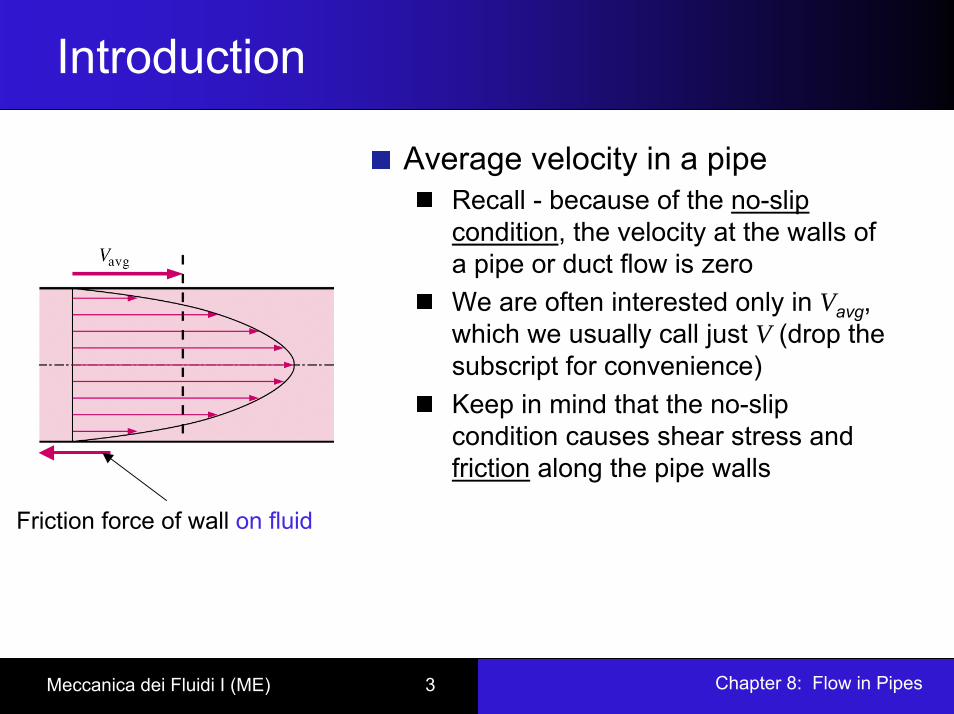
Average velocity in a pipeRecall - because of the no-slip condition, the velocity at the walls of a pipe or duct flow is zeroWe are often interested only in Vavg, which we usually call just V (drop the subscript for convenience)Keep in mind that the no-slip condition causes shear stress and friction along the pipe walls
Friction force of wall on fluid

Chapter 8: Flow in PipesMeccanica dei Fluidi I (ME) 4
Introduction
For pipes of constant diameter and incompressible flow
Vavg stays the same down the pipe, even if the velocity profile changes
Why? Conservation of Mass
Vavg Vavg
samesame
same
Chapter 8: Flow in PipesMeccanica dei Fluidi I (ME) 5
Introduction
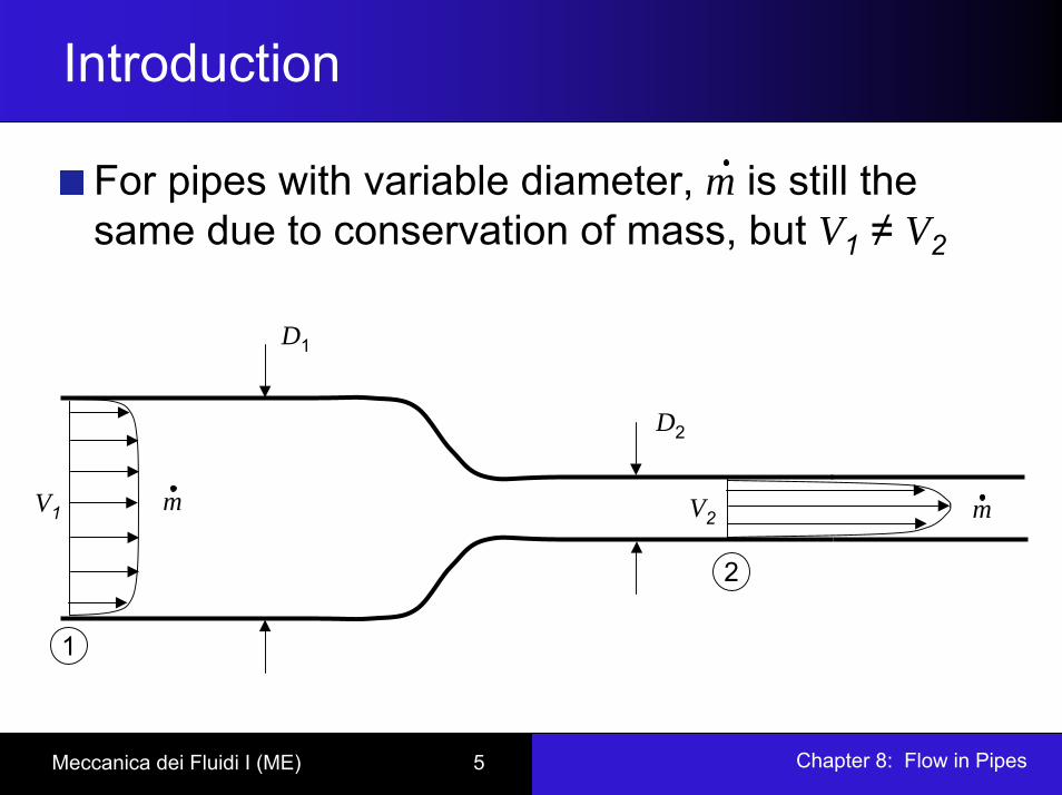
For pipes with variable diameter, m is still the same due to conservation of mass, but V1 ≠ V2
D2
2
V2
1
V1
D1
m m

Chapter 8: Flow in PipesMeccanica dei Fluidi I (ME) 6
Laminar and Turbulent Flows
Inertial forcesViscous forces
Clay Institute Millennium Prize
Re =
Chapter 8: Flow in PipesMeccanica dei Fluidi I (ME) 7
Laminar and Turbulent Flows
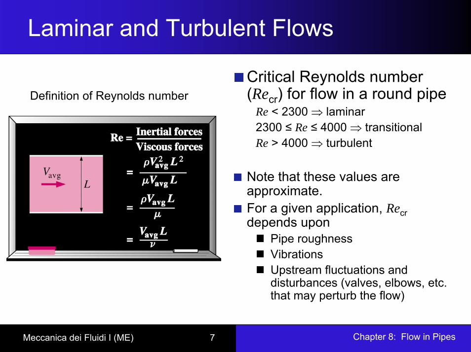
Critical Reynolds number (Recr) for flow in a round pipe
Re < 2300 ⇒ laminar2300 ≤ Re ≤ 4000 ⇒ transitional Re > 4000 ⇒ turbulent
Note that these values are approximate.For a given application, Recrdepends upon
Pipe roughnessVibrationsUpstream fluctuations and disturbances (valves, elbows, etc. that may perturb the flow)
Definition of Reynolds number

Chapter 8: Flow in PipesMeccanica dei Fluidi I (ME) 8
Osborne Reynolds (1842-1912)
Chapter 8: Flow in PipesMeccanica dei Fluidi I (ME) 9
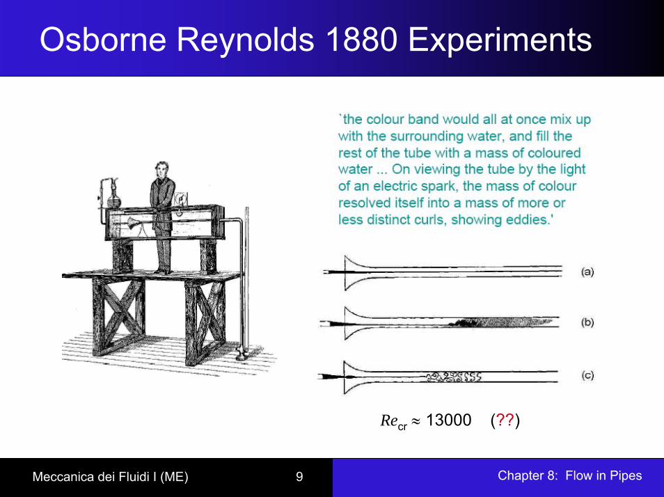
Osborne Reynolds 1880 Experiments
Recr ≈ 13000 (??)
Chapter 8: Flow in PipesMeccanica dei Fluidi I (ME) 10
Laminar and Turbulent Flows
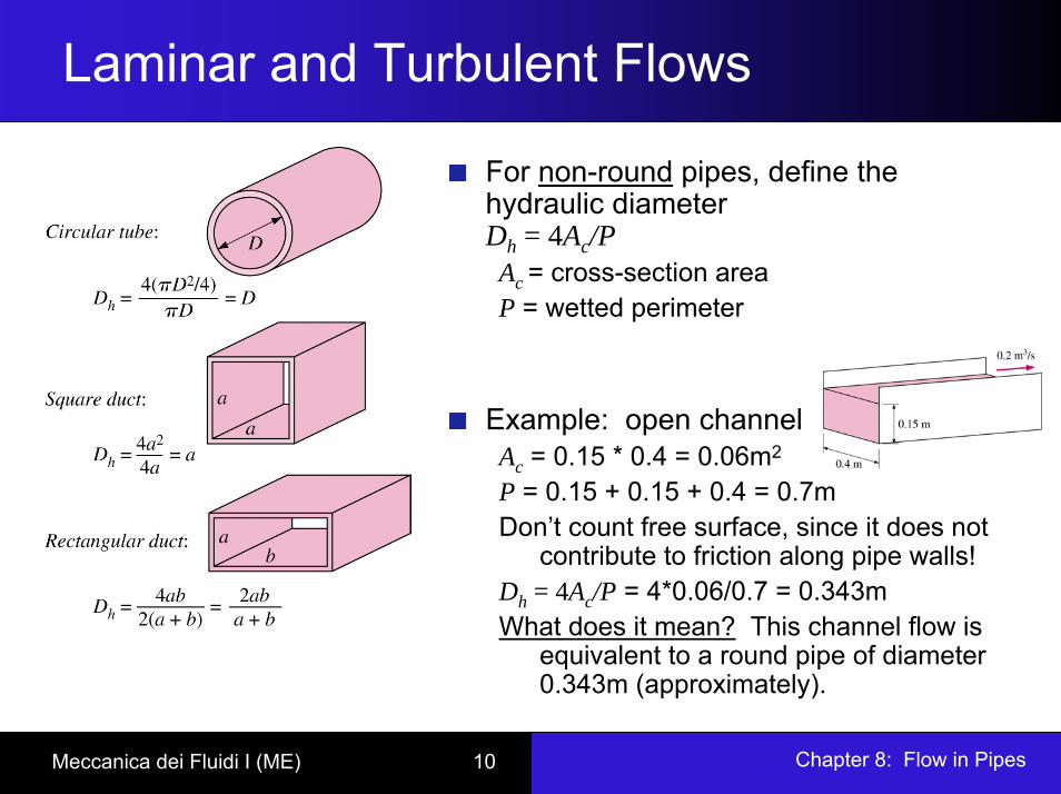
For non-round pipes, define the hydraulic diameter Dh = 4Ac/PAc = cross-section areaP = wetted perimeter
Example: open channelAc = 0.15 * 0.4 = 0.06m2
P = 0.15 + 0.15 + 0.4 = 0.7mDon’t count free surface, since it does not
contribute to friction along pipe walls!Dh = 4Ac/P = 4*0.06/0.7 = 0.343mWhat does it mean? This channel flow is
equivalent to a round pipe of diameter 0.343m (approximately).
Chapter 8: Flow in PipesMeccanica dei Fluidi I (ME) 11
The Entrance Region
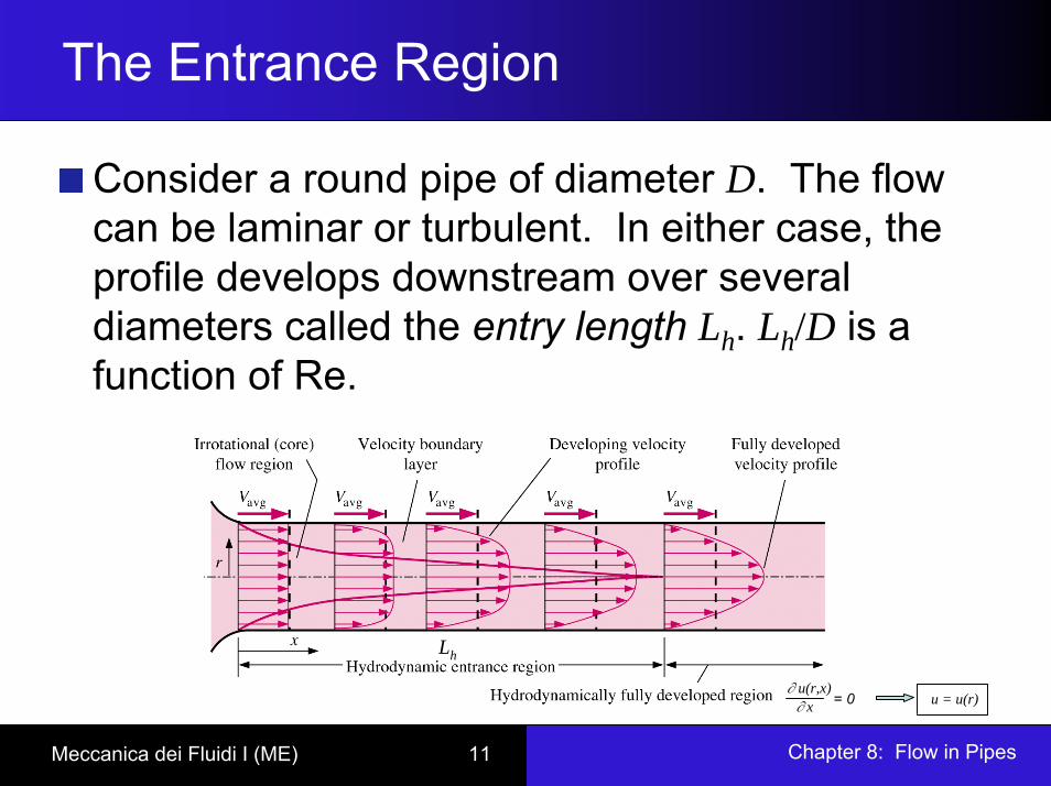
Consider a round pipe of diameter D. The flow can be laminar or turbulent. In either case, the profile develops downstream over several diameters called the entry length Lh. Lh/D is a function of Re.
Lh
∂ u(r,x)∂ x = 0 u = u(r)
Chapter 8: Flow in PipesMeccanica dei Fluidi I (ME) 12
Fully Developed Pipe Flow
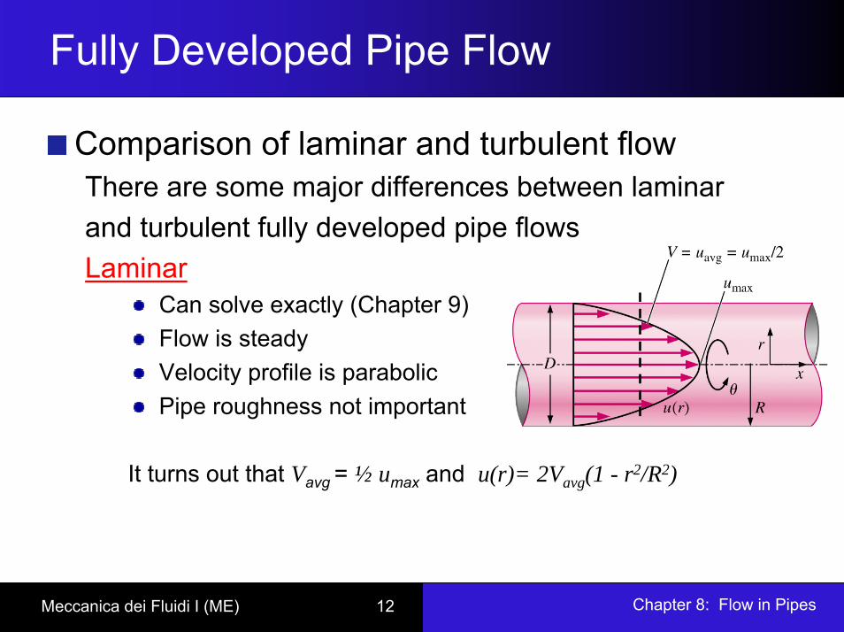
Comparison of laminar and turbulent flowThere are some major differences between laminar and turbulent fully developed pipe flowsLaminar
Can solve exactly (Chapter 9)Flow is steadyVelocity profile is parabolicPipe roughness not important
It turns out that Vavg = ½ umax and u(r)= 2Vavg(1 - r2/R2)
Chapter 8: Flow in PipesMeccanica dei Fluidi I (ME) 13
Fully Developed Pipe Flow
= − µ du/dr
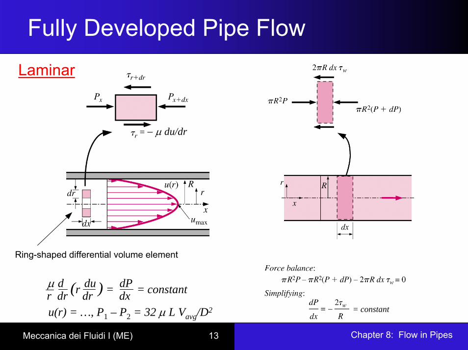
Laminar
= constant
Ring-shaped differential volume element
µ d du dPr dr dr dx(r ) = = constant
u(r) = …, P1 – P2 = 32 µ L Vavg/D2
Chapter 8: Flow in PipesMeccanica dei Fluidi I (ME) 14
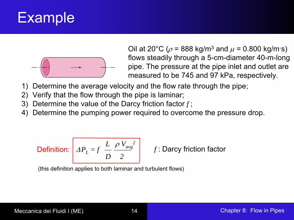
Example
1) Determine the average velocity and the flow rate through the pipe;2) Verify that the flow through the pipe is laminar;3) Determine the value of the Darcy friction factor f ;4) Determine the pumping power required to overcome the pressure drop.
Oil at 20°C (ρ = 888 kg/m3 and µ = 0.800 kg/m.s)flows steadily through a 5-cm-diameter 40-m-longpipe. The pressure at the pipe inlet and outlet aremeasured to be 745 and 97 kPa, respectively.
Definition: ∆PL = fL ρ Vavg
2
D 2f : Darcy friction factor
(this definition applies to both laminar and turbulent flows)
Chapter 8: Flow in PipesMeccanica dei Fluidi I (ME) 15
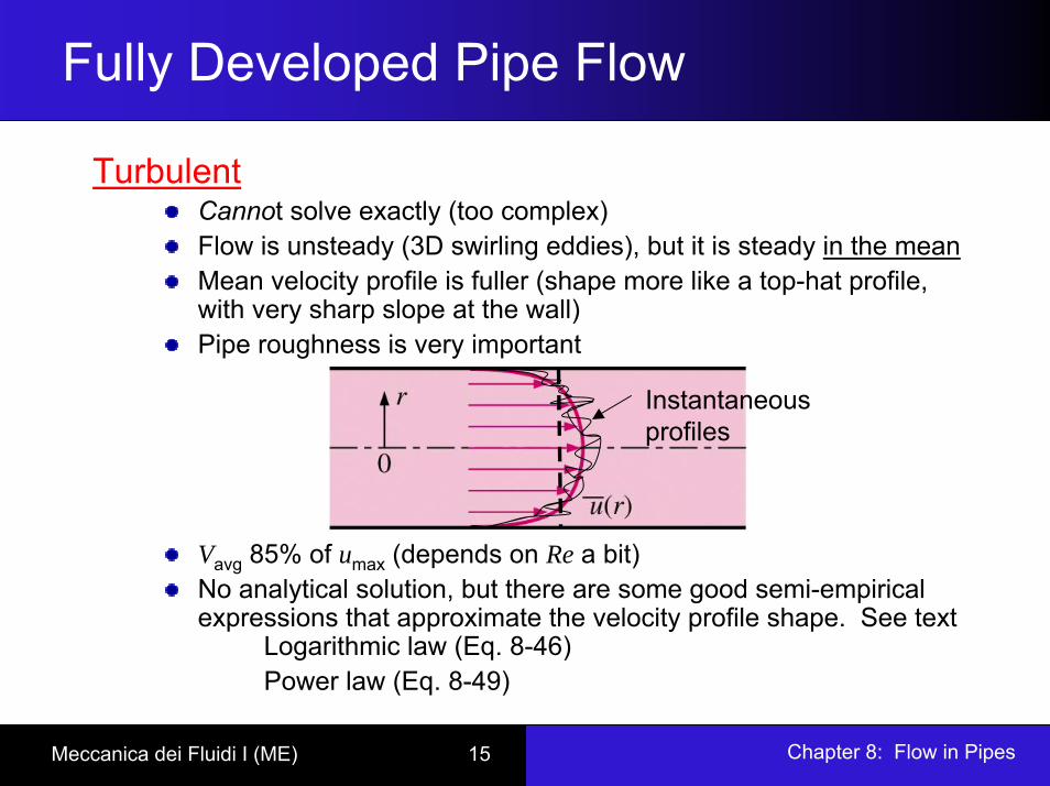
Fully Developed Pipe Flow
TurbulentCannot solve exactly (too complex)Flow is unsteady (3D swirling eddies), but it is steady in the meanMean velocity profile is fuller (shape more like a top-hat profile, with very sharp slope at the wall) Pipe roughness is very important
Vavg 85% of umax (depends on Re a bit)No analytical solution, but there are some good semi-empirical expressions that approximate the velocity profile shape. See text
Logarithmic law (Eq. 8-46)Power law (Eq. 8-49)
Instantaneousprofiles

Chapter 8: Flow in PipesMeccanica dei Fluidi I (ME) 16
Fully Developed Pipe Flow Wall-shear stress
Recall, for simple shear flows u=u(y), we had τ = µ du/dy
In fully developed pipe flow, it turns out thatτ = -µ du/dr
slope
slope
Laminar Turbulent
τw τw
τw,turb > τw,lamτw = shear stress at the wall,
acting on the fluid
Chapter 8: Flow in PipesMeccanica dei Fluidi I (ME) 17
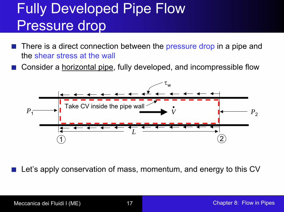
Fully Developed Pipe Flow Pressure drop
There is a direct connection between the pressure drop in a pipe and the shear stress at the wallConsider a horizontal pipe, fully developed, and incompressible flow
Let’s apply conservation of mass, momentum, and energy to this CV
1 2L
τw
P1 P2VTake CV inside the pipe wall

Chapter 8: Flow in PipesMeccanica dei Fluidi I (ME) 18
Fully Developed Pipe Flow Pressure drop
Conservation of Mass
Conservation of x-momentum
Terms cancel since β1 = β2and V1 = V2
Chapter 8: Flow in PipesMeccanica dei Fluidi I (ME) 19
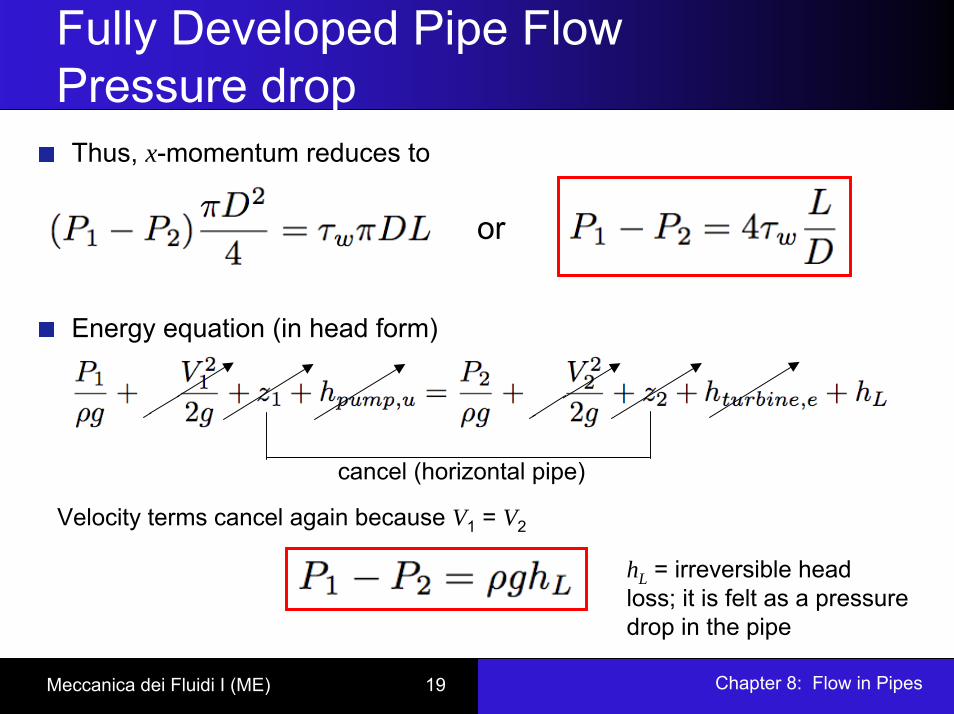
Fully Developed Pipe Flow Pressure drop
Thus, x-momentum reduces to
Energy equation (in head form)
or
cancel (horizontal pipe)
Velocity terms cancel again because V1 = V2
hL = irreversible head loss; it is felt as a pressuredrop in the pipe
Chapter 8: Flow in PipesMeccanica dei Fluidi I (ME) 20
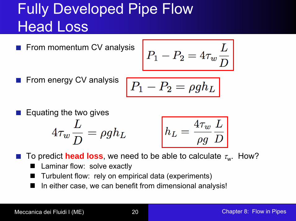
Fully Developed Pipe Flow Head Loss
From momentum CV analysis
From energy CV analysis
Equating the two gives
To predict head loss, we need to be able to calculate τw. How?Laminar flow: solve exactlyTurbulent flow: rely on empirical data (experiments)In either case, we can benefit from dimensional analysis!
Chapter 8: Flow in PipesMeccanica dei Fluidi I (ME) 21
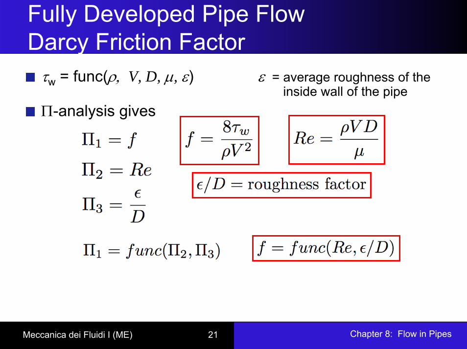
Fully Developed Pipe Flow Darcy Friction Factor
τw = func(ρ, V, D, µ, ε) ε = average roughness of the inside wall of the pipe
Π-analysis gives

Chapter 8: Flow in PipesMeccanica dei Fluidi I (ME) 22
Fully Developed Pipe Flow Friction Factor
Now go back to equation for hL and substitute f for τw
Our problem is now reduced to solving for Darcy friction factor f
RecallTherefore
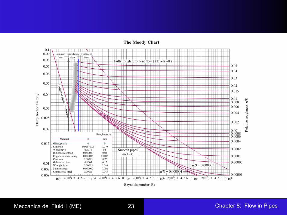
Laminar flow: f = 64/Re (exact)Turbulent flow: Use charts or empirical equations (Moody Chart, a famous plot of f vs. Re and ε/D)
But for laminar flow, roughness does not affect the flow unless it is huge
Chapter 8: Flow in PipesMeccanica dei Fluidi I (ME) 23
Chapter 8: Flow in PipesMeccanica dei Fluidi I (ME) 24
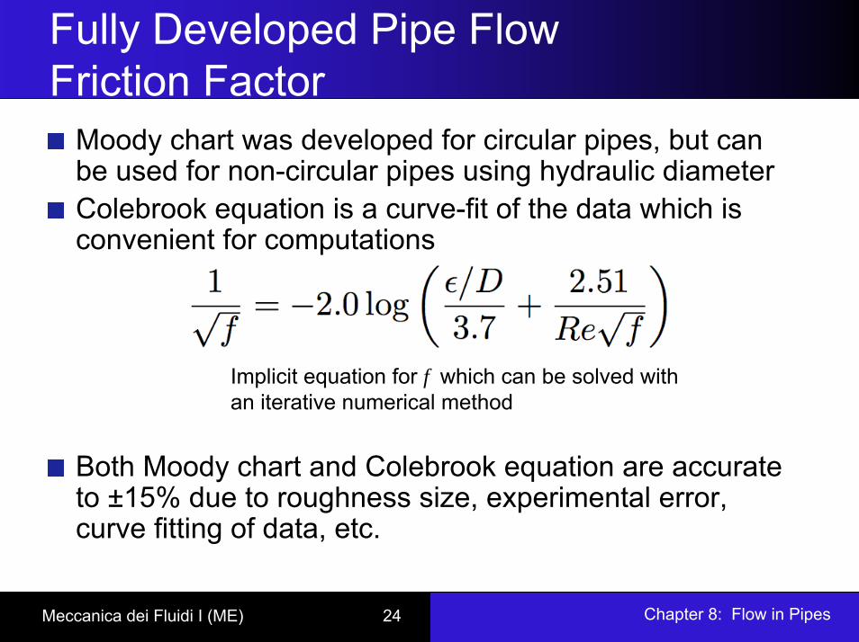
Fully Developed Pipe Flow Friction Factor
Moody chart was developed for circular pipes, but can be used for non-circular pipes using hydraulic diameterColebrook equation is a curve-fit of the data which is convenient for computations
Both Moody chart and Colebrook equation are accurate to ±15% due to roughness size, experimental error, curve fitting of data, etc.
Implicit equation for f which can be solved with an iterative numerical method

Chapter 8: Flow in PipesMeccanica dei Fluidi I (ME) 25
Types of Fluid Flow Problems
In design and analysis of piping systems, 3 problem types are encountered
1. Determine ∆p (or hL) given L, D, V (or flow rate)Can be solved directly using Moody chart and Colebrook equation
2. Determine V, given L, D, ∆p3. Determine D, given L, ∆p, V (or flow rate)Types 2 and 3 are common engineering design problems, i.e., selection of pipe diameters to minimize construction and pumping costs. However, iterative approach required since both V and D are in the Reynolds number.
Chapter 8: Flow in PipesMeccanica dei Fluidi I (ME) 26
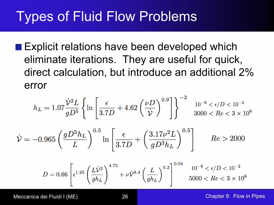
Types of Fluid Flow Problems
Explicit relations have been developed which eliminate iterations. They are useful for quick, direct calculation, but introduce an additional 2% error

Chapter 8: Flow in PipesMeccanica dei Fluidi I (ME) 27
Example
Heated air at 1 atm and 35°C is to be transported in a 150-m–long circular plastic duct at a rate of 0.35 m3/s. If the head loss in the pipe is not to exceed 20 m, determine the maximum required pumping power, the minimum diameter of the duct, average velocity, the Reynolds number and the Darcy friction factor.
ρ = 1.145 kg/m3, ν = 1.655 10-5 m2/s
Chapter 8: Flow in PipesMeccanica dei Fluidi I (ME) 28
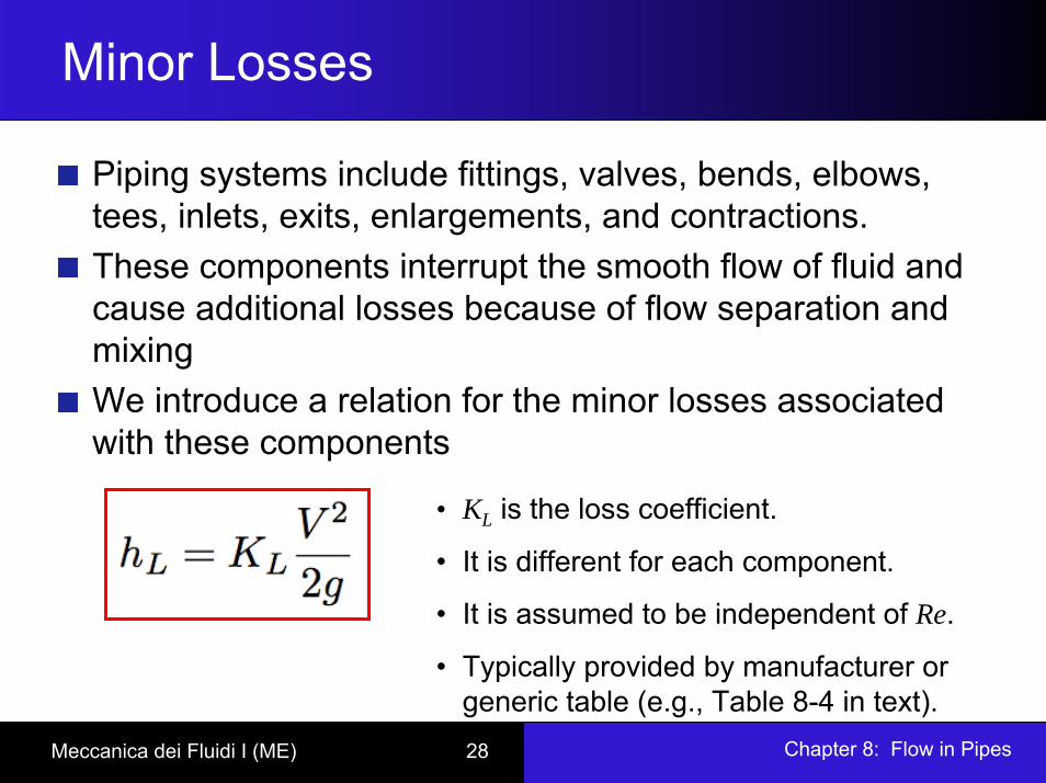
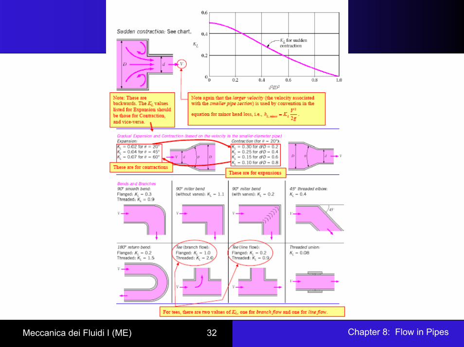
Minor Losses
Piping systems include fittings, valves, bends, elbows, tees, inlets, exits, enlargements, and contractions.These components interrupt the smooth flow of fluid and cause additional losses because of flow separation and mixingWe introduce a relation for the minor losses associated with these components
• KL is the loss coefficient.
• It is different for each component.
• It is assumed to be independent of Re.
• Typically provided by manufacturer or generic table (e.g., Table 8-4 in text).
Chapter 8: Flow in PipesMeccanica dei Fluidi I (ME) 29
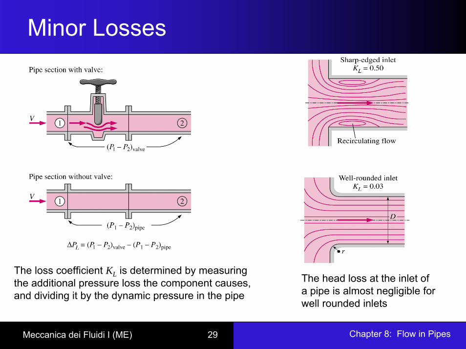
Minor Losses
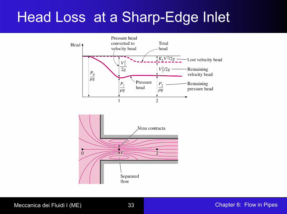
The loss coefficient KL is determined by measuringthe additional pressure loss the component causes,and dividing it by the dynamic pressure in the pipe
The head loss at the inlet ofa pipe is almost negligible forwell rounded inlets
Chapter 8: Flow in PipesMeccanica dei Fluidi I (ME) 30
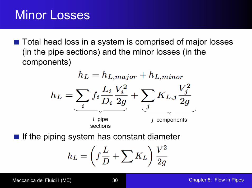
Minor Losses
Total head loss in a system is comprised of major losses (in the pipe sections) and the minor losses (in the components)
If the piping system has constant diameter
i pipe sections
j components

Chapter 8: Flow in PipesMeccanica dei Fluidi I (ME) 31
α = 2 for fully developed laminar flow
α ≈ 1 for fully developed turbulent flow
Chapter 8: Flow in PipesMeccanica dei Fluidi I (ME) 32
Chapter 8: Flow in PipesMeccanica dei Fluidi I (ME) 33
Head Loss at a Sharp-Edge Inlet

Chapter 8: Flow in PipesMeccanica dei Fluidi I (ME) 34
Example
A 9-cm-diameter horizontal water pipe contracts gradually to a 6-cm-diameter pipe. The walls of the contraction section are angled 30° fromthe horizontal. The average velocity and pressure of water at the exit ofthe contraction section are 7 m/s and 150 kPa, respectively. Determine the head loss in the contraction section and the pressure in the larger-diameter pipe.
12
Turbulent fully developed flow at sections 1 and 2, ρ = 1000 kg/m3, KL ?
Chapter 8: Flow in PipesMeccanica dei Fluidi I (ME) 35
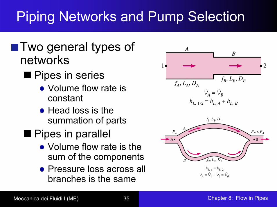
Piping Networks and Pump Selection
Two general types of networks
Pipes in seriesVolume flow rate is constantHead loss is the summation of parts
Pipes in parallelVolume flow rate is the sum of the componentsPressure loss across all branches is the same

Chapter 8: Flow in PipesMeccanica dei Fluidi I (ME) 36
Piping Networks and Pump Selection
For parallel pipes, perform CV analysis between points A and B
Since ∆ P is the same for all branches, head loss in all branches is the same

Chapter 8: Flow in PipesMeccanica dei Fluidi I (ME) 37
Piping Networks and Pump Selection
Head loss relationship between branches allows the following ratios to be developed
so that the relative flow rates in parallel pipes are established from the requirements that the head loss in each pipe is the same
Real pipe systems result in a system of non-linear equations. Note: the analogy with electrical circuits should be obvious
Flow rate (V ): current (I)Pressure gradient (∆p): electrical potential (V)Head loss (hL): resistance (R), however hL is very nonlinear
.

Chapter 8: Flow in PipesMeccanica dei Fluidi I (ME) 38
Piping Networks and Pump Selection
When a piping system involves pumps and/or turbines, pump and turbine head must be included in the energy equation
The useful head of the pump (hpump,u) or the head extracted by the turbine (hturbine,e), are functions of volume flow rate, i.e., they are not constants.Operating point of system is where the system is in balance, e.g., where pump head is equal to the head loss (plus elevation difference, velocity head difference, etc.)
Chapter 8: Flow in PipesMeccanica dei Fluidi I (ME) 39
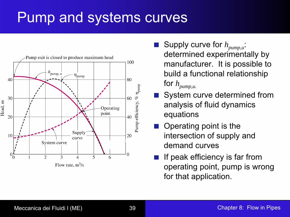
Pump and systems curves
Supply curve for hpump,u: determined experimentally by manufacturer. It is possible to build a functional relationship for hpump,u.
System curve determined from analysis of fluid dynamics equationsOperating point is the intersection of supply and demand curvesIf peak efficiency is far from operating point, pump is wrong for that application.