Chapter 7 Time-varying Electromagnetic Fields

Displacement Current, Maxwell’s EquationsBoundary Conditions, Potential Function

Energy Flow Density, Time-harmonic Electromagnetic Fields Complex Vector Expressions

1. Displacement Electric Current 2. Maxwell’s Equations 3. Boundary Conditions for Time-varying Electromagnetic Fields 4. Scalar and Vector Potentials 5. Solution of Equations for Potentials 6. Energy Density and Energy Flow Density Vector 7. Uniqueness Theorem 8. Time-harmonic Electromagnetic Fields 9. Complex Maxwell’s Equations 10. Complex Potentials 11. Complex Energy Density and Energy Flow Density Vector

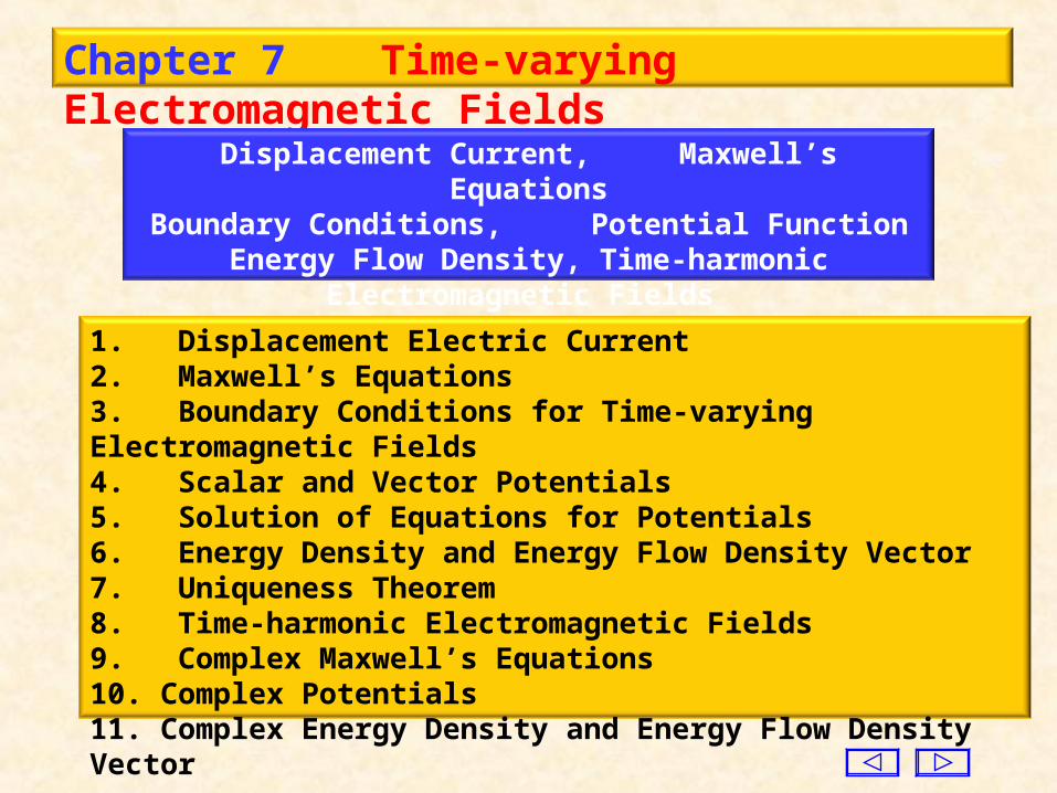
1. Displacement Electric Current

The displacement current is neither the conduction current nor the

convection current, which are formed by the motion of electric

charges. It is a concept given by J. C. Maxwell.

For static fields 0d S SJ 0 J

Based on the principle of electric charge conservation, we have

t

qS

SJ d

t

J

which are called the continuity equations for electric

current.

For time-varying electromagnetic fields, since the charges are

changing with time, the electric current continuity principle cannot be

derived from static considerations. Nevertheless, an electric current is

always continuous. Hence an extension of earliest concepts for steady

current need to be developed.

Gauss’ law for electrostatic fields, , is still valid for time-

varying electric fields, we obtain

qS

d SD

0d

SS

t

DJ

The current in a vacuum capacitor is

neither the conduction current nor the

convection current, but it is actually the

displacement electric current.

Obviously, the dimension of is the same as that of the current

density.tD

0

t

DJ

t

D

Jd

0d)( d S

SJJ 0)( d JJWe obtain

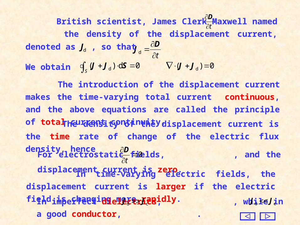
British scientist, James Clerk Maxwell named the density of the

displacement current, denoted as Jd , so thattD

The introduction of the displacement current makes the time-

varying total current continuous, and the above equations are called

the principle of total current continuity.

The density of the displacement current is the time rate of change

of the electric flux density, hence

For electrostatic fields, , and the displacement current is zero. 0

t

D

In time-varying electric fields, the displacement current is larger if

the electric field is changing more rapidly.

In imperfect dielectrics, , while in a good conductor, . cd JJ cd JJ

Maxwell considered that the displacement current must also produce

magnetic fields, and it should be included in the Ampere circuital law, so

thatSJJlH d)(d

d Sl

SD

JlH d)(d

Sl t t

D

JHi.e.

Which are Ampere’s circuital law with the displacement current. It

shows that a time-varying magnetic field is produced by the conduction

current, the convection current, and the displacement current.

The displacement current, which results from time-varying electric

field, produces a time-varying magnetic field.

Maxwell deduced the coexistence of a time-varying electric field and

a time-varying magnetic field, and they result in an electromagnetic

wave in space. This prediction was demonstrated in 1888 by Hertz.

The law of electromagnetic induction shows that a time-varying

magnetic field can produce a time-varying electric field.

2. Maxwell’s Equations

For the time-varying electromagnetic field, Maxwell summarized

the following four equations:

SD

JlH d)(d

Sl t

SB

lE dd

Sl t

0d

S SB

qS

d SD

The integral form

t

D

JH

t

BE

0 B

D

The differential form

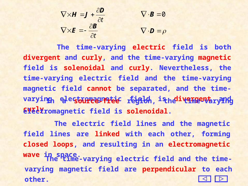
The time-varying electric field is both divergent and curly, and the

time-varying magnetic field is solenoidal and curly. Nevertheless, the

time-varying electric field and the time-varying magnetic field cannot

be separated, and the time-varying electromagnetic field is divergent

and curly.

In a source-free region, the time-varying electromagnetic field is

solenoidal.

The electric field lines and the magnetic field lines are linked with

each other, forming closed loops, and resulting in an electromagnetic

wave in space.

The time-varying electric field and the time-varying magnetic field

are perpendicular to each other.

t

D

JH

t

BE

0 B

D

In order to describe more completely the behavior of time-varying

electromagnetic fields, Maxwell’s equations need to be supplemented by

the charge conservation equation and the constitutive relations:

t

J ED HB JEJ

The four Maxwell’s equations are not independent. Equations 4 and

3 can be derived from Equation 1 and 2, respectively, and vise versa.

For static fields, we have

0

tttt

BHDE

Maxwell’s equations become the former equations for electrostatic

field and steady magnetic field. Furthermore, the electric field and the

magnetic field are independent each other.

where stands for the impressed source producing the time-varying

electromagnetic field.

J

“These equations are the laws representing the structure of the

field. They do not, as in Newton’s laws, connect two widely separated

events; they do not connect the happenings here with the conditions

there”.

As the founder of relativity, Albert Einstein (1879-1955), pointed

out in his book “The Evolution of Physics” that

“The field here and now depends on the field in the immediate

neighborhood at a time just past. The equations allow us to predict

what will happen a little further in space and a little later in time, if we

know what happens here and now”

“The formulation of these equations is the most important event in

physics since Newton’s time, and they are the quantitative

mathematical description of the laws of the field. Their content is much

richer than we have been able to indicate, and the simple form conceals

a depth revealed only by careful study”.

Maxwell’s equations have made important impact on the

history of mankind, besides the advancement of science and

technology.

As American physicist, Richard P. Feynman, said in his book

“The Feynman Lectures on Physics”, that “From along view of the

history of mankind──seen from say, ten thousand years from now

──there can be little doubt that the most significant event of the 19-

th century will be judged as Maxwell’s discovery of the laws of

electrodynamics. The American civil war will pale into provincial

insignificance in comparison with this important scientific event of

the same decade.”

In this information age, from baby monitor to remote-controlled

equipment, from radar to microwave oven, from radio broadcast to

satellite TV, from ground mobile communication to space communi-

cation, from wireless local area network to blue tooth technology,

and from global positioning to navigation systems, electromagnetic

waves are used as to make these technologies possible.

To appreciate the contributions Maxwell and Hertz have made to

the progress of mankind and our culture, one only needs to look at

the wide usage of electromagnetic waves.

The wireless information highway makes it possible that we can

reach anybody anywhere at anytime, and to be able to send text,

voice, or video signals to the recipient miles away. Electromagnetic

waves can recreate the experience of events far away, making

possible wireless virtual reality.

3. Boundary Conditions for Time-varying Electromagnetic Fields

In principle, all boundary conditions satisfied by a static field can be

applied to a time-varying electromagnetic field.

(a) The tangential components of the electric field intensity are

continuous at any boundary, i.e.

As long as the time rate of change of the magnetic flux density is

finite, using the same method as before we can obtain it from the

equation:

2t1t EE

or 0)( 12n EEe

SB

lE dd

Sl t

For linear isotropic media, the above equation can be rewritten as

2

t2

1

t1

DD

①

② en

(b) The normal components of magnetic flux intensity are

continuous at any boundary.

From the principle of magnetic flux continuity, we find

2nn1 BB

or 0)( 12n BBe

(c) The boundary condition for the normal components

of electric flux density depends on the property of the media.

In general, from Gauss’ law we find

SDD 1n2n

or S )( 12n DDe

where S is the surface density of the free charge at the boundary.

For linear isotropic media, we have n22 n11 HH

At the boundary between two perfect dielectrics, because of the

absence of free charges, we have

2n1n DD

(d) The boundary condition for the tangential components of the

magnetic field intensity depends also on the property of the media.

In general, in the absence of surface currents at the boundary, as

long as the time rate of change of the electric flux density is finite, we

find t21t HH

0)( 12n HHeor

However, surface currents can exist on the surface of a perfect

electric conductor, and in this case the tangential components of the

magnetic field intensity are discontinuous.

For a linear isotropic dielectric, we have 2n2 n11 EE

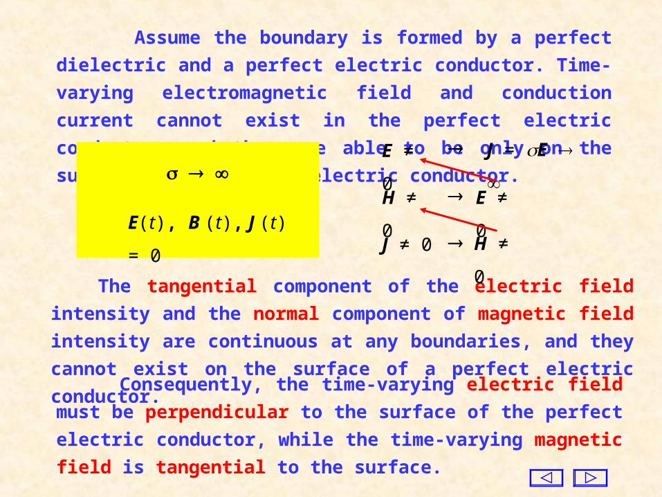
Assume the boundary is formed by a perfect dielectric and a

perfect electric conductor. Time-varying electromagnetic field and

conduction current cannot exist in the perfect electric conductor, and

they are able to be only on the surface of the perfect electric

conductor.

The tangential component of the electric field intensity and the

normal component of magnetic field intensity are continuous at any

boundaries, and they cannot exist on the surface of a perfect electric

conductor.

E(t), B (t), J (t) = 0

E ≠ 0 J = E

H ≠ 0 E ≠ 0

J ≠ 0 H ≠ 0

Consequently, the time-varying electric field must be perpendicular

to the surface of the perfect electric conductor, while the time-varying

magnetic field is tangential to the surface.

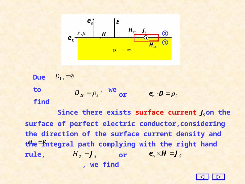
Due to ， we find 01n D

SD 2n or SDen

Since there exists surface current JS on the surface of perfect

electric conductor,considering the direction of the surface current

density and the integral path complying with the right hand rule,

, we find01t H

SH J2t SJHe nor

E

H ,

en

et ①②

H1t

H2t JS

Example. The components of the time-varying electromagnetic

field in a rectangular metal waveguide of interior cross-section a b

are

) sin(π

cos0 zktxa

HH zzz

) cos(π

sin0 zktxa

HH zxx

) cos(π

sin0 zktxa

EE zyy

Find the density of the

displacement current in

the waveguide and the

charges and the currents

on the interior walls of the

waveguide. The inside is

vacuum.

a

z

y

x

b

x

z y

x

y

z

g

b

a

Magnetic field lines Electric field lines

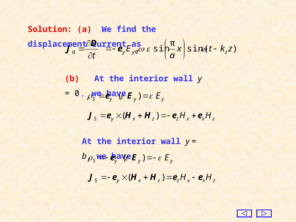
Solution: (a) We find the displacement current as

t

D

Jd ) sin(π

sin 0 zktxa

E zyy

e

(b) At the interior wall y = 0 ， we

have yyyS E ) ( Ee

zxxzzxyS HH eeHHeJ )(

At the interior wall y = b, we have

yyyS E ) ( Ee

zxxzzxyS HH eeHHeJ )(

At the lateral wall x = 0 , , we have0xH

) sin() sin( 00 zktHzktH zzyzzzxS eeeJ

) sin()) sin(( 00 zktHzktH zzyzzzxS eeeJ

At the lateral wall x = a , , we find 0xH

At the lateral walls x = 0 and x = a, due to , and . 0yE 0S

z

y

x

The currents on the interior walls

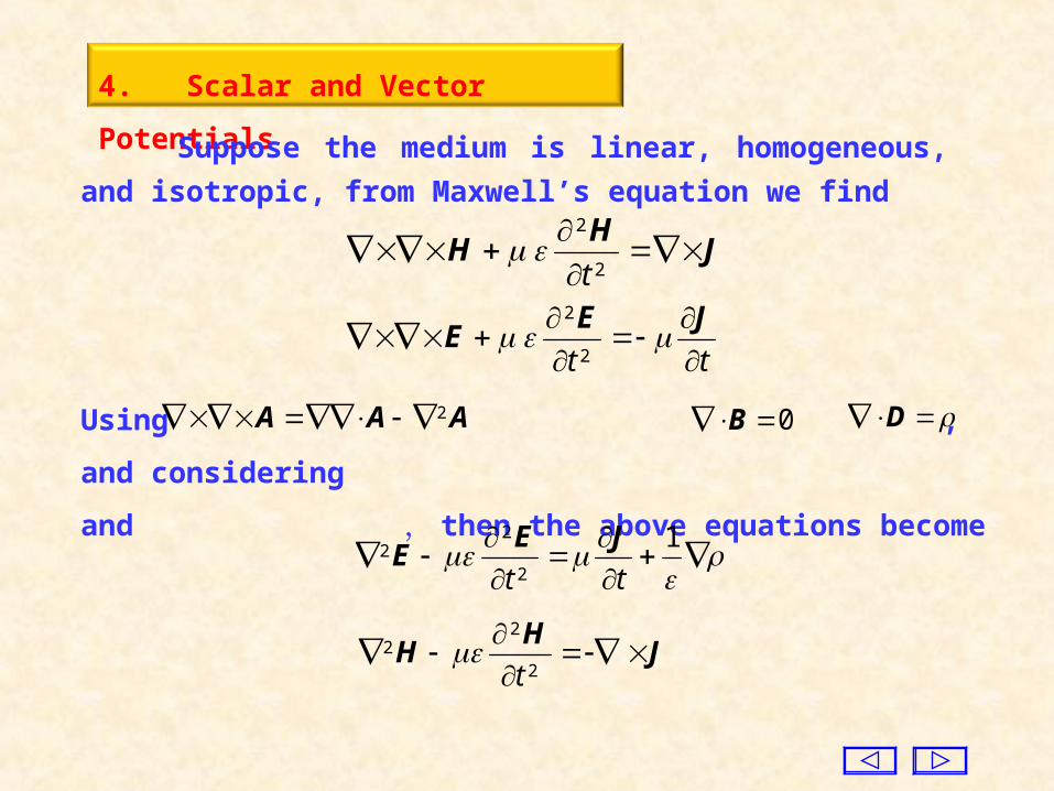
4. Scalar and Vector Potentials

JH

H

2

2

t

Suppose the medium is linear, homogeneous, and isotropic,

from Maxwell’s equation we find

tt

JE

E 2

2

Using , and considering

and ， then the above equations become

0 BAAA 2 D

JH

H

2

22

t

1

2

22

tt

JEE

JH

H

2

22

t

1

2

22

tt

JEE

The relationship between the field intensities and the sources is

quite complicated. To simplify the process, it will be helpful to solve

the time-varying electromagnetic fields by introducing two auxiliary

functions: the scalar and the vector potentials.

AB

where A is called the vector potential. Substituting the above equation

into givest

BE

)( AE

t

Due to , hence B can be expressed in terms of the curl of

a vector field A, as given by

0 B

The above equation can be rewritten as 0

t

AE

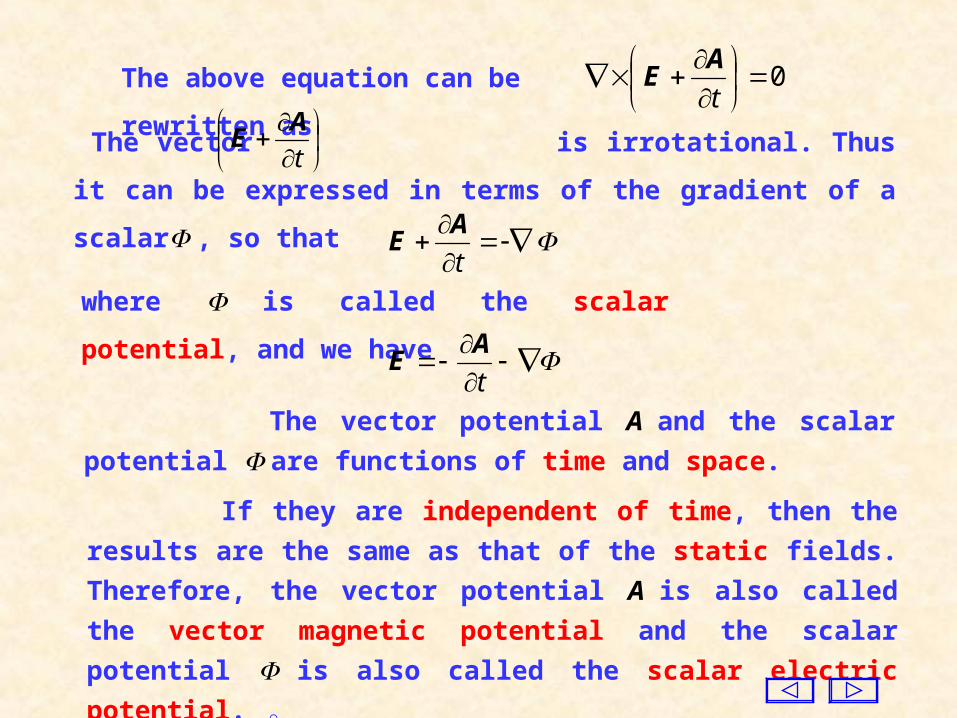
The vector is irrotational. Thus it can be expressed in terms of

the gradient of a scalar , so that

t

AE

t

AE

where is called the scalar potential, and we have

t

AE

The vector potential A and the scalar potential are functions of

time and space.

If they are independent of time, then the results are the same as

that of the static fields. Therefore, the vector potential A is also called

the vector magnetic potential and the scalar potential is also called

the scalar electric potential. 。

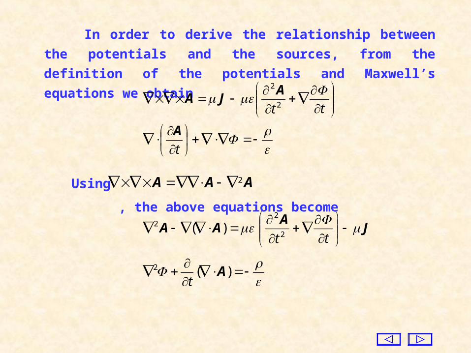
In order to derive the relationship between the potentials and the

sources, from the definition of the potentials and Maxwell’s equations

we obtain

t

tt

A

AJA

2

2

JA

AA

tt 2

22 )(

)(2 At

Using , the above equations becomeAAA 2

The curl of the vector field A is given as , but the divergence

must be specified.

BA

t

Φ

A

Then the above two equations become

JA

A 2

22

t

2

22

t

ΦΦ

Lorentz condition

After the divergence of the vector potential A is given by the

Lorentz condition, the equations are simplified. The original equations

are two coupled equations, while new equations are decoupled.

In principle, the divergence can be taken arbitrarily, but to simplify

the application of the equations, we can see that if let

The vector potential A only depends on the current J, while the scalar

potential is related to the charge density only.

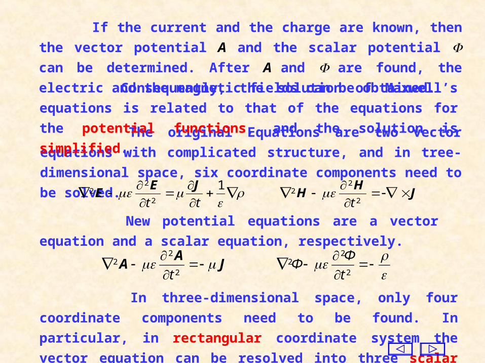
If the current and the charge are known, then the vector potential A

and the scalar potential can be determined. After A and are found,

the electric and the magnetic fields can be obtained.

The original Equations are two vector equations with complicated

structure, and in tree-dimensional space, six coordinate components

need to be solved.

New potential equations are a vector equation and a scalar

equation, respectively.

JH

H

2

22

t

1

2

22

tt

JEE

Consequently, the solution of Maxwell’s equations is related to that

of the equations for the potential functions, and the solution is

simplified.

In three-dimensional space, only four coordinate components need

to be found. In particular, in rectangular coordinate system the vector

equation can be resolved into three scalar equations。

JA

A 2

22

t

2

22

t

ΦΦ

Here we find the solution by using an analogous method based on

the results of static fields.

5. Solution of Equations for Potentials

If the source is a time-varying point charge placed at the origin, the

distribution of the field should be a function of the variable r only, and

independent of the angles and .

The scalar potential caused by a point charge is obtained first, then

use superposition principle to obtain the solution of the scalar potential

due to a distribution of time-varying charge.

rt

r

vr

r0 0

) (1) (2

2

22

2

1

vwhere

In the open space excluding the origin, the scalar potential function

satisfies the following equation

The above equation is the homogeneous wave equation for the

function ( r), and the general solution is

v

rtf

v

rtfr 21

We will know that the second term is contrary to the physical

situation, and it should be excluded. Therefore, we find the scalar

electric potential as

rvr

tftΦ

1

),(r

The electric potential produced by the static elemental charge

at the origin isVq d

r

V

π4

d )(

r

Comparing the above two equations, we

know

Vvr

t

v

rtf d

π4

1

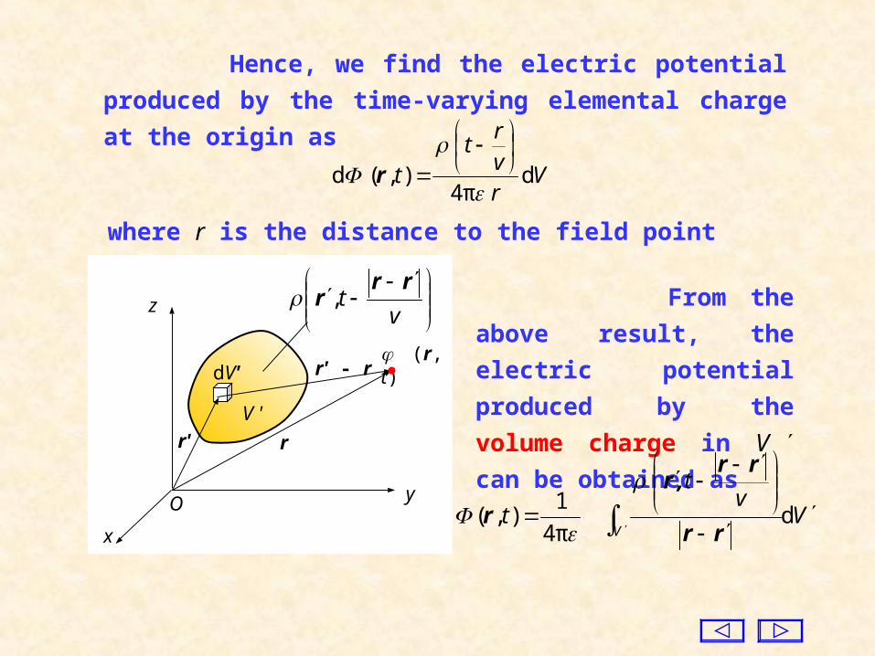
Hence, we find the electric potential produced by the time-

varying elemental charge at the origin as

Vrvr

tt d

π4

),( d

r

where r is the distance to the field point from the charge dV .

From the above result,

the electric potential produced

by the volume charge in V can be obtained as

Vv

t

tV

dπ4

1),(

rr

rr,r

r

r' r

z

y

x

(r, t)

V '

dV'

vt

rrr ,

r' - r

O

To find the vector potential function A, the above equation can

be expanded in rectangular coordinate system, with all coordinate

components satisfying the same inhomogeneous wave equation, i.e.

x

xx J

t

AA

2

22

yy

y Jt

AA

2

22

zz

z Jt

AA

2

22

Apparently, for each component we can find a solution similar

to that of scalar potential equation. Incorporating the three

components gives the solution of the vector potential A as

Vv

t

tV

d

,

π4),(

rr

rrrJ

rA

Vv

t

tV

dπ4

1),(

rr

rr,r

r

V

vt

tV

d

,

π4),(

rr

rrrJ

rA

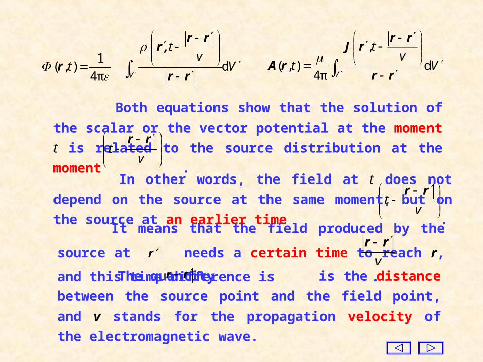
Both equations show that the solution of the scalar or the

vector potential at the moment t is related to the source distribution

at the moment .

vt

rr

It means that the field produced by the source at r needs a

certain time to reach r, and this time difference is . v

rr

vt

rr In other words, the field at t does not depend on the source at the

same moment, but on the source at an earlier time .

The quantity is the distance between the source point

and the field point, and v stands for the propagation velocity of the

electromagnetic wave.

rr

From we can see that the propagation velocity of

electromagnetic wave is related to the properties of the medium. In

vacuum,

1

v

m/s103m/s2997924581 8

00

v

which is the propagation velocity of light in vacuum, also called the

speed of light, usually denoted as c.

It is worth noting that the field at a point away from the source

may still be present at a moment after the source ceases to exist.

Energy released by a source travels away from the source and

continuous to propagate even after the source is taken away. This

phenomenon is a consequence of electromagnetic radiation.

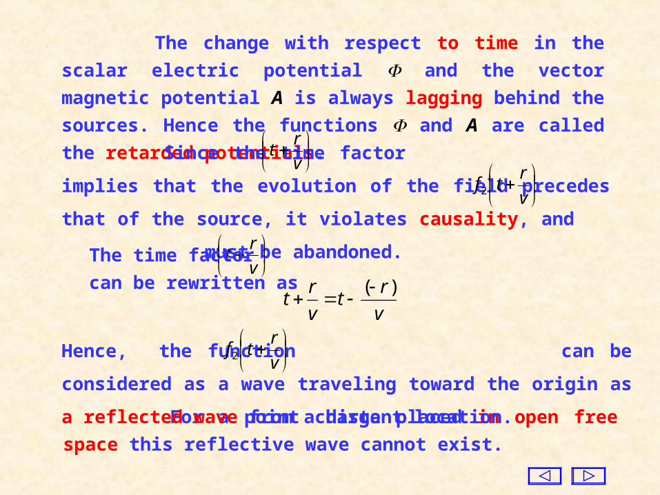
The change with respect to time in the scalar electric potential

and the vector magnetic potential A is always lagging behind the

sources. Hence the functions and A are called the retarded

potentials.

Since the time factor implies that the evolution of the

field precedes that of the source, it violates causality, and

must be abandoned.

v

rtf2

v

rt

v

rtThe time factor can be rewritten as

v

rt

v

rt

)(

For a point charge placed in open free space this reflective wave

cannot exist.

Hence, the function can be considered as a wave traveling

toward the origin as a reflected wave from a distant location.

v

rtf2

For surface or line charge and current, consider the following

substitutions:

All of the above equations are valid only for linear,

homogeneous, and isotropic media.

lSV lS ddd lJJ ddd ISV S

S

S

Sv

t

t d

,

π4

1),(

rr

rrr

r

S

S

Sv

t

t d

,

π4),(

rr

rrrJ

rA

l

l

lv

t

t d

,

π4

1),(

rr

rrr

r

l

lv

tI

t d

,

π4),(

rr

rrr

rA

We obtain

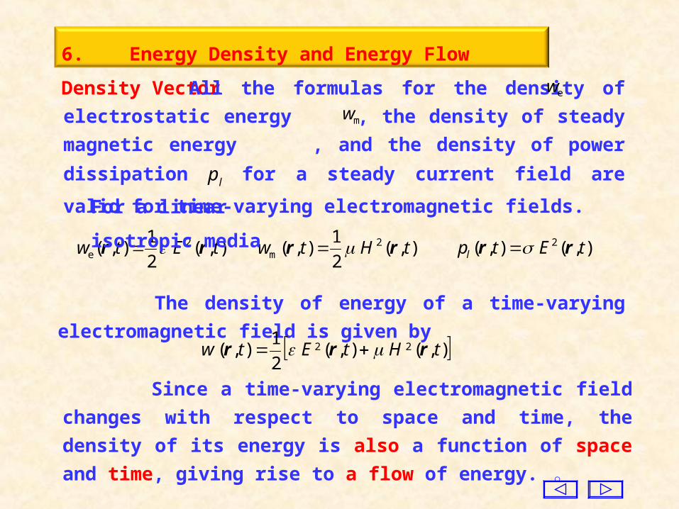
6. Energy Density and Energy Flow Density Vector

),( 2

1),( 2

e tEtw rr ),( 2

1),( 2

m tHtw rr ),( ),( 2 tEtpl rr

The density of energy of a time-varying electromagnetic field is

given by ),( ),(

2

1),( 22 tHtEtw rrr

For a linear isotropic media

Since a time-varying electromagnetic field changes with respect to

space and time, the density of its energy is also a function of space and

time, giving rise to a flow of energy. 。

All the formulas for the density of electrostatic energy , the

density of steady magnetic energy , and the density of power

dissipation pl for a steady current field are valid for time-varying

electromagnetic fields.

mwew

t

E

EH

t

H

E

0) ( H

0) ( E

Using , we haveHEEHHE )(

222

2

2

)( E

E

t

H

t

HE

Integrating both sides of the equation over the volume V, we have

V V V

VEVHEt

V

222 d d) (2

1d)( HE

, ,

E, HV

Suppose there is a linear isotropic medium in the region V

without any impressed source , and the parameters of

the medium are . Then in this region the electromagnetic

field satisfies the following Maxwell’s equations:

)0 0( ,J , ,

Considering , we have V S

V

d)(d)( SHEHE

V VS

VHEt

VE

222

d) (

2

1d d)( SHE

Based on the definition of energy density, the above equation

can be rewritten as

V lSV

VpVwt

dd )(d SHE

which is called the energy theorem for time-varying electromagnetic

field, and any time-varying electromagnetic field satisfying Maxwell’s

equation must obey the energy theorem. The vector ( ) represents

the power passing through

unit cross-sectional area and

that is just the energy flow

density vector S, given by

HE

, ,

E, H

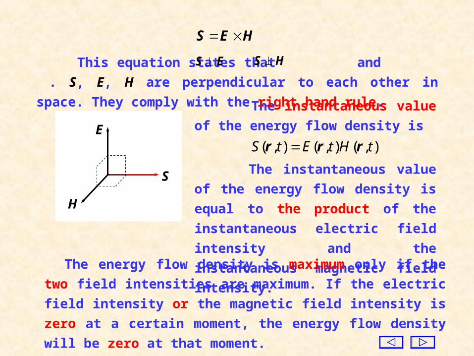
HES

S

HES

S

E

H

The instantaneous value of the energy

flow density is

),(),(),( tHtEtS rrr

The instantaneous value of the energy

flow density is equal to the product of the

instantaneous electric field intensity and

the instantaneous magnetic field intensity.

The energy flow density is maximum only if the two field intensities

are maximum. If the electric field intensity or the magnetic field

intensity is zero at a certain moment, the energy flow density will be

zero at that moment.

This equation states that and . S, E, H are perpendicular

to each other in space. They comply with the right hand rule.

ES HS

7. Uniqueness Theorem

In a region V bound by a closed surface S, if the initial values of the

electric field intensity E and the magnetic field intensity H are given at

the time t = 0, as long as the tangential component Et of the electric field

intensity or the tangential component Ht of the magnetic field intensity

is given at the boundary for t > 0, then the electromagnetic field will be

uniquely determined by Maxwell’s equations at any moment t (t > 0) in

the region V.

Based on the energy theorem and using the method of contrary,

this theorem can be proved.

V

SE t (r, t) or H t (r, t)

E(r, 0)&

H(r, 0 )

E( r, t), H(r, t )

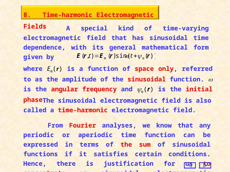
8. Time-harmonic Electromagnetic Fields

A special kind of time-varying electromagnetic field that has

sinusoidal time dependence, with its general mathematical form

given by))( sin()(),( em rrErE tt

where Em(r) is a function of space only, referred to as the amplitude

of the sinusoidal function. is the angular frequency and e(r) is the

initial phase.

From Fourier analyses, we know that any periodic or

aperiodic time function can be expressed in terms of the sum of

sinusoidal functions if it satisfies certain conditions. Hence, there is

justification for us to concentrate on sinusoidal electromagnetic

fields.

The sinusoidal electromagnetic field is also called a time-

harmonic electromagnetic field.

A sinusoidal electromagnetic field is produced by charge and

current that have sinusoidal time dependence. The time dependence

of the field is the same as that of the source in a linear medium.

Thus the field and the source of a sinusoidal electromagnetic field

have the same frequency.

The electric field intensity can be expressed in terms of a

complex vector as)(m rE)(j

mmee )()( rrErE

The original instantaneous vector can be expressed in terms of

the complex vector as

]e )(Im[),( jm

tt rErE

A complex vector can be used to represent these sinusoidal

quantities with the same frequency. Namely, only the amplitude

and the space phase are considered, while the time

dependent part is omitted.

)(e r

t

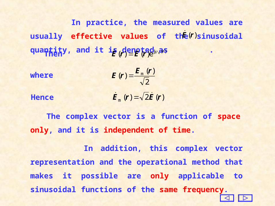
In practice, the measured values are usually effective values

of the sinusoidal quantity, and it is denoted as .)(rE

2

)()( m rE

rE where

)(2)(m rErE Hence

The complex vector is a function of space only, and it is

independent of time.

In addition, this complex vector representation and the

operational method that makes it possible are only applicable to

sinusoidal functions of the same frequency.

)(j ee)()( rrErE Then

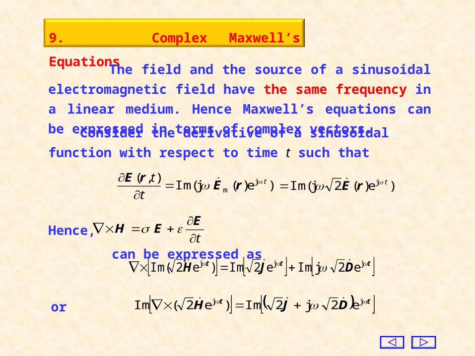
9. Complex Maxwell’s Equations

The field and the source of a sinusoidal electromagnetic field

have the same frequency in a linear medium. Hence Maxwell’s

equations can be expressed in terms of complex vectors.

)e)( jIm(),( j

mt

t

t rErE

)e)(2jIm( j t rE

Consider the derivative of a sinusoidal function with respect to

time t such that

ttt DJH jjj e2 jIme2Im)e2Im(

tt DJH jj e2 j2Im)e2(Im or

Hence, can be expressed ast

E

EH

In the same way, we find

BE j

0 B

D

j J

ED HB

JEJ

and

The above equations are called Maxwell’s equations in the

frequency domain, with all field variables being complex.

Since the above equation holds for any moment t, the

imaginary symbol can be eliminated.

DJH 2 j22 DJH j

tt DJH jj e2 j2Im)e2(Im

Example. The instantaneous value of the electric field intensity

of a time-variable electromagnetic field in vacuum is

) sin() π10sin(2),( zktxt zy erE

Find complex magnetic field intensity.

Solution: From the instantaneous value we have the complex

vector of the electric field intensity as zk

yzx je) π10sin()( erE

Since the electric field has only the y-component, and it is

independent of the variable y, so that , then0

y

E y

x

E

z

E yz

yx

eeE zk

zzk

zxzz xxk jj e ) π10cos( π10e) π10sin(j ee

Due to HBE 0jj EH 0

j

zkz

zx

zxxk j

0 0

e) π10cos(

π10j) π10sin(

eeHWe find

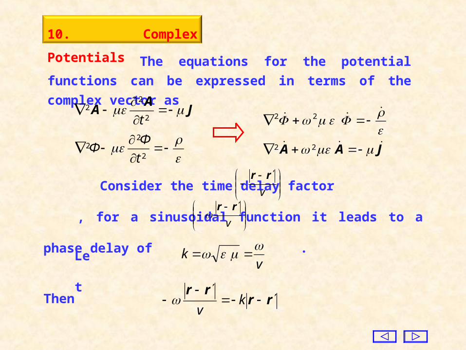
10. Complex Potentials

The equations for the potential functions can be expressed in

terms of the complex vector as

Consider the time delay factor , for a sinusoidal

function it leads to a phase delay of .

v

rr

v

rr

Letv

k

rrrr

kv

Then

JA

A 2

22

t

2

22

t

ΦΦ JAA 22

22

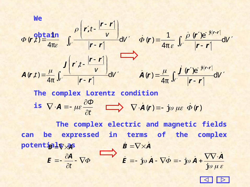
We obtain

The complex Lorentz condition is

The complex electric and magnetic fields can be expressed in

terms of the complex potentials as

Vv

t

tV

dπ4

1),(

rr

rr,r

r

Vv

t

tV

d

,

π4),(

rr

rrrJ

rA

VV

k

de)(

π4)(

j

rr

rJrA

r-r

VV

k

de)(

π4

1)(

j

rr

rr

r-r

t

Φ

A )( j)( rrA

t

AE

AB AB

j j j

AAAE

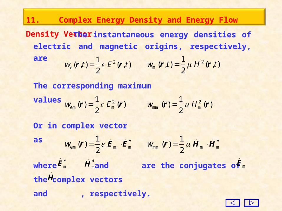
11. Complex Energy Density and Energy Flow Density Vector

The instantaneous energy densities of electric and magnetic

origins, respectively, are

),( 2

1),( 2

e tEtw rr ),( 2

1),( 2

m tHtw rr

The corresponding maximum values

)( 2

1)( 2

mem rr Ew )( 2

1)( 2

mmm rr Hw

*EEr mmem 2

1)( w *HHr mmmm

2

1)( w

Or in complex vector as

where and are the conjugates of the complex vectors

and , respectively.

*Em *Hm

mE

mH

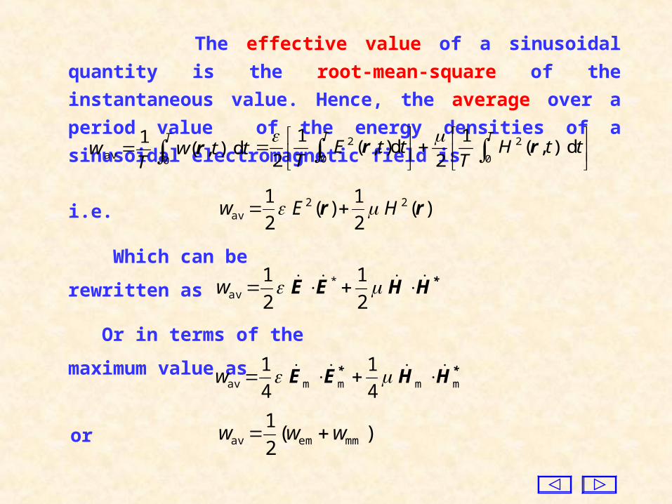
The effective value of a sinusoidal quantity is the root-mean-

square of the instantaneous value. Hence, the average over a period

value of the energy densities of a sinusoidal electromagnetic field is

ttwT

wT

d ),(1

0 av r

ttH

TttE

T

TTd ),(

1

2d),(

1

2

0

2

0

2 rr

)( 2

1)(

2

1 22av rr HEw i.e.

Or in terms of the maximum value as

** HHEE mmmmav 4

1

4

1 w

)(2

1mmemav www or

*HHEE 2

1

2

1 *av w

Which can be rewritten as

)(2

1mmemav www

which states that the average value of the energy density of a sinusoidal

electromagnetic field is equal to half of the sum of the maximum values

of the electric energy density and the magnetic energy density.

Similarly, the power dissipation per unit volume can also be

expressed in terms of the complex vector, and the maximum value is

*EErr mm2mm )()( Epl

*mm

2av

2

1 )( )( EEEErr * Ep l

The time average is

The time average of the power dissipation per unit volume is also

the half of the maximum value.

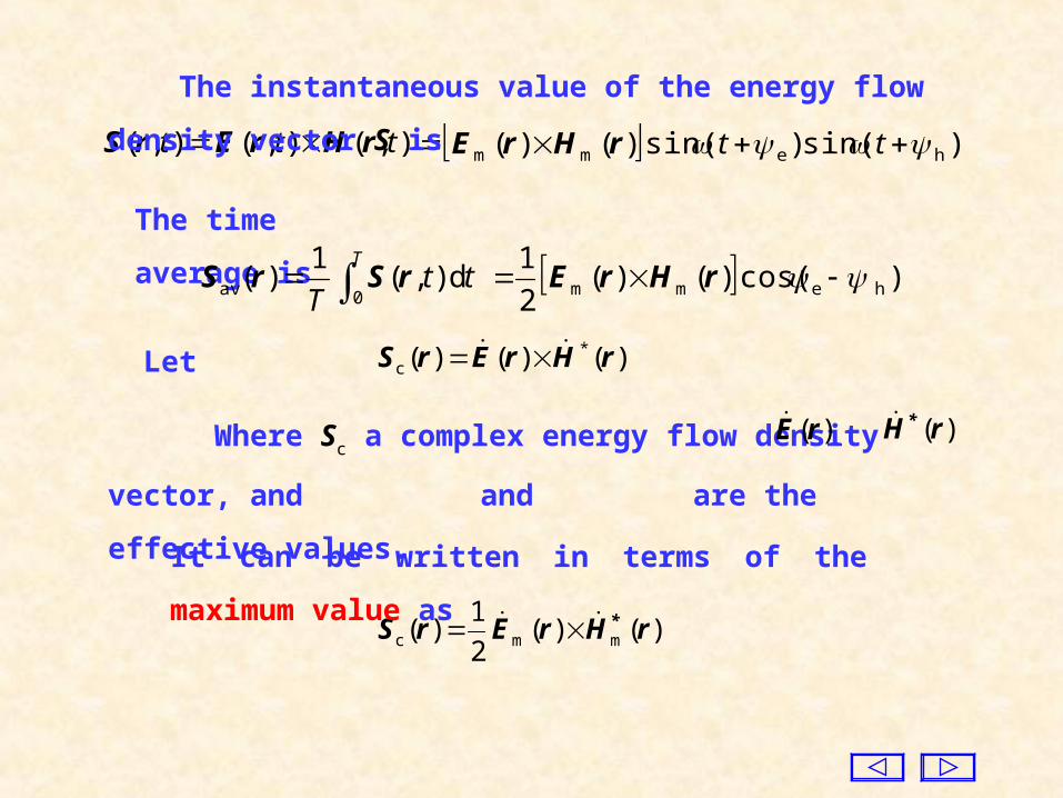
),(),(),( ttt rHrErS ) sin() sin()()( hemm ttrHrE

The instantaneous value of the energy flow density vector S is

The time average is

ttT

Td ),(

1)(

0 av rSrS )cos()()(2

1h emm rHrE

Where Sc a complex energy flow density vector, and and

are the effective values.

)(rE )(rH *

)()(2

1)( mmc rHrErS *

It can be written in terms of the maximum value as

)()()( *c rHrErS Let

Then the real part and the imaginary part of the complex energy

flow density vector Sc, are

)cos()()(2

1)Re( hemmc rHrES

)sin()()(2

1)Im( hemmc rHrES

we can see that the real part of the complex energy flow density

vector is just the time average of the energy flow density vector, i.e.

)()Re( avc rSS

The real part and the imaginary part of the complex energy flow

density vector depend not only on the magnitudes of the electric and

the magnetic fields but also on the phases.

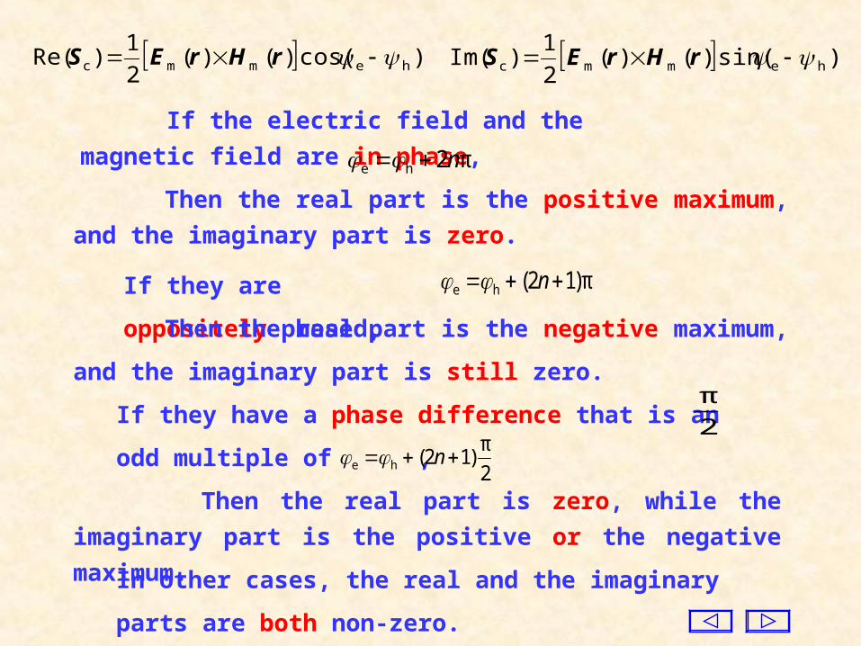
If the electric field and the magnetic field are in phase,

π2he n

If they are oppositely

phased,

π)12(he n

If they have a phase difference that is an odd multiple of , 2

π

2

π)12(he n

)cos()()(2

1)Re( hemmc rHrES )sin()()(

2

1)Im( hemmc rHrES

In other cases, the real and the imaginary parts are both non-zero.

Then the real part is the positive maximum, and the imaginary

part is zero.

Then the real part is the negative maximum, and the imaginary

part is still zero.

Then the real part is zero, while the imaginary part is the positive

or the negative maximum.

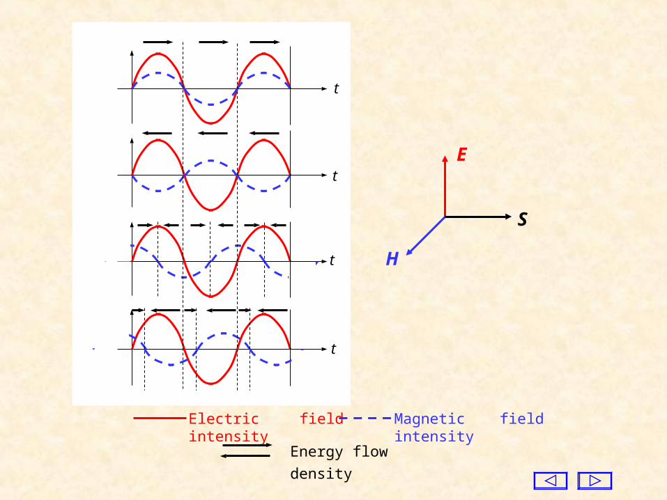
Electric field intensity Magnetic field intensity

t

t

t

t

Energy flow density

E

H

S

V

V

V

VS

d) ( j

d d)(

*

**

*

EEHH

EESHE

The energy theorem can also be expressed by complex vectors as

Vww

V

V

V lS

d )()(2 j

d )( d)(

eavmav

c

rr

rPSrS

i.e.

which is called the complex energy

theorem. The real part of the flux of complex energy flow density vector

flowing into the closed surface S is equal to the power dissipation

within the closed surface. It shows clearly that the real part of Sc

stands for the energy flowing along a certain direction.

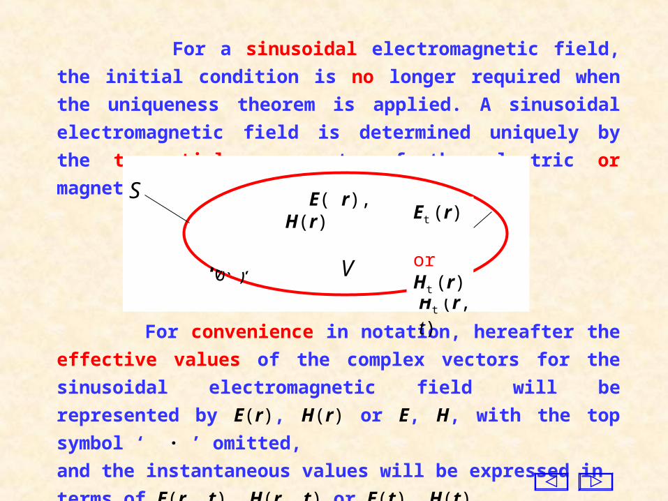
For convenience in notation, hereafter the effective values of the

complex vectors for the sinusoidal electromagnetic field will be

represented by E(r), H(r) or E, H, with the top symbol ‘ · ’ omitted,

and the instantaneous values will be expressed in terms of E(r, t), H(r,

t) or E(t), H(t) .

For a sinusoidal electromagnetic field, the initial condition is no

longer required when the uniqueness theorem is applied. A sinusoidal

electromagnetic field is determined uniquely by the tangential

components of the electric or magnetic fields at the boundary.

V

SE(r, 0)

&H(r, 0 )

E( r, t), H(r, t ) E( r), H(r)Et (r, t) orHt (r, t)

Et (r) orHt (r)

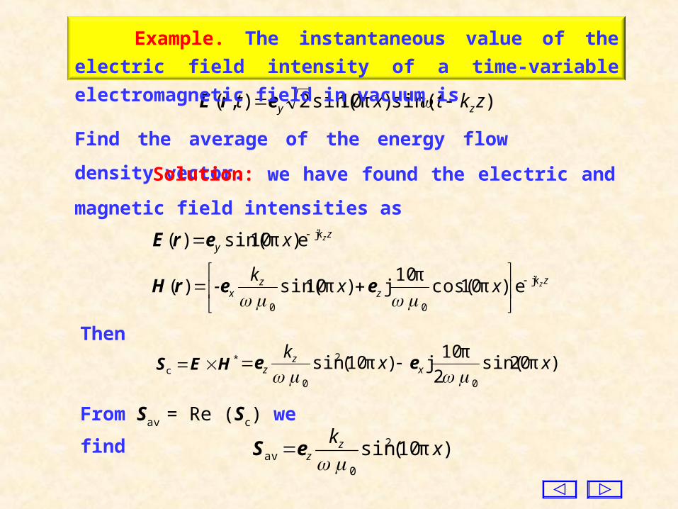
) sin() π10sin(2),( zktxt zy erE

Find the average of the energy flow density vector.

Solution: we have found the electric and magnetic field

intensities as

Example. The instantaneous value of the electric field intensity

of a time-variable electromagnetic field in vacuum is

From Sav = Re (Sc) we find

*c HES ) π20sin(

2

π10j) π10(sin

0

2

0

xxk

xz

z ee

Then

) π10(sin

2

0 av x

kzz

eS

zkz

zx

zxxk

- j

0 0

e) π10cos(

π10j) π10sin(

)(

eerH

zky

zx je) π10sin()( erE