Chapter 7 - Results and Discussion

7 .1 Introduction 7 .1

7 .2 Probe Measurements of Magnetic Field 7 .2

7 .3 Langmuir Probes 7 .11

7 .4 Microwave Interferometer 7 .12

7 .5 Interpretation of Spectrosco?icMeasurements

7 .17

7 .6 Discussion 7 .23

7 .7 Possible Studies Arising from this Work 7 .34

7 .1

Introduction

From the shapes of the wave fields presented later in this chapter,

it can be seen that 0 :e coil structure surrounding the vacuum vessel does

in fact excite a helicon wave . It will be shown that for a constant gas

pressure, increasing the magnetic field Bc :_ increased the degree of ionization

by greater than an order of magnitude . . The helicon wave fields are obviously

interacting strongly with the electrons which acquire considerable energy,

sufficient to ionize the neutral atoms . Formally, then, the problem is far

from being linear With the wave fields causing considerable perturbation

to the plasma parameters, and the linear theory presented in chapter 3,

section 5 is a very approximate model to the actual situation .

Before presenting the experimental results, a phenomenological

description of the plasma will be given for a constant neutral gas pressure

of 1 .5 millitorr and changing B0

.

When Bo is less than about 381) gauss, the plasma exhibits the

characteristic pink glow of the low ionized positive column of Argon .

Magnetic probe measurements show that for Bo L 50 gauss the radial field

components are all of about the same magnitude

The average density

suddenly increases at Bo ti 180 gauss and the wavelength becomes less than

the impressed wavelength . Between 180 and 380 gauss tha average density

increases linearly with Bo but the wave gradually develops a much longer

wavelength component . A sudden change in average density at 380 gauss

is associated with the longer wavelength component becoming dominant

although a much shorter low amplitude component of the wavelength can still

be measured .

The plasma is then a light blue colour

7 .1

7 .2

due to excitation of All lines, implying a greater number of excited ions

radiating . The wavelength slowly decreases asBo

is further increased

until at about 750 gauss the wavelength suddenly decreases to be approxi-

mately the same wavelength as that impressed by the R .F . coil, accompanied

by another large increase in the density .

In this final mode, the plasma has a very peaked density distribu-

tion which shows as a bright blue central core . The b e and b r fields are

about an order of magnitude greater than the b z field at these higher

average densities and wave fields

The experimental data presented below were taken in these regions

with special attention- paid- to the - two- sudden - changes in . wavelength and

plasma parameters . All experiments were carried out at 8 .6 MHz .

7 .2

Probe Measurements of Magnetic Field

As the plasma being investigated was formed by the interaction of

the wave fields and currents with the electrons of the plasma, the effect

of inserting a finite sized cold Pyrex tube into the plasma needed to be

known . As a first check, the gas pressure, magnetic field Bo and power

into the plasma were kept constant while a probe was pushed axially into

the plasma at a distance 3 cm from the central axis . The probe was oriented

to measure the bz component of the wave which was recorded every 2 cm

over an axial distance of 90 cm from the top of the vacuum tube . This

probe was then withdrawn and the bz

component outside the plasma, but

along a line parallel to the previous set of measurements, was determined

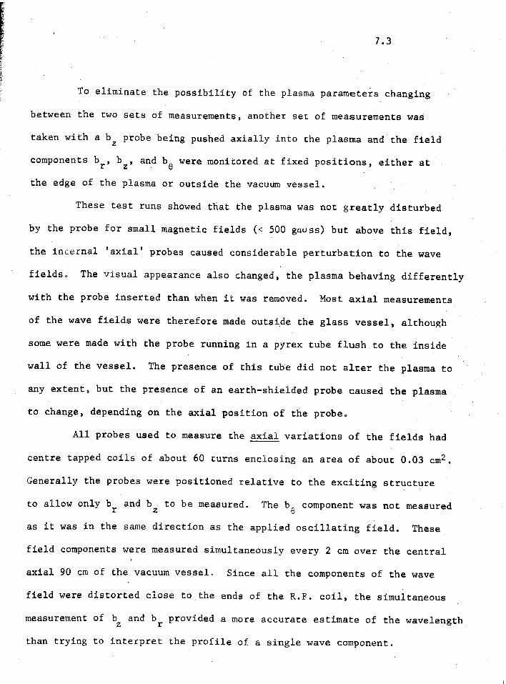
To eliminate the possibility of the plasma parameters changing

between the two sets of measurements, another set of measurements was

taken with a b Z probe being pushed axially into the plasma and the field

components br , b Z , and b e were monitored at fixed positions, either at

the edge of the plasma or outside the vacuum vessel .

These test runs showed that the plasma was not greatly disturbed

by the probe for small magnetic fields (< 500 gauss) but above this field,

the internal 'axial' probes caused considerable perturbation to the wave

fields . The visual appearance also changed, the plasma behaving differently

with the probe inserted than when it was removed . Most axial measurements

of the wave fields were therefore made outside the glass vessel, although

some were made with the probe running in a pyrex tube flush to the inside

wall of the vessel . The presence of this tube did not alter the plasma to

any extent, but the presence of an earth-shielded probe caused the plasma

to change, depending on the axial position of the probe .

All probes used to measure the axial variations of the fields had

centre tapped coils of about 60 turns enclosing an area of about 0 .03 cm2 .

Generally the probes were positioned relative to the exciting structure

to allow only b r and b Z to be measured . The b e component was not measured

as it was in the same direction as the applied oscillating field . These

field components were measured simultaneously every 2 cm over the central

axial 90 cm of the vacuum vessel . Since all the components of the wave

field were distorted close to the ends of the R .F . coil, the simultaneous

measurement of bZ and b r provided a more accurate estimate of the wavelength

than trying to interpret the profile of a single wave component .

7 . 3

B0 (gauss) ( m) ak

47 56 0.56

103 56 0 .56

188 35 0 .90

226 32 0 .98

282 32 0 .98

385 64 04q

507 64 C :49

602 64 0 .49

696 62 0 .51

800 51 0 .62

7 .4

As mentioned before, the probes were very susceptible to electro-

static pickup (and also to breakage)' and although the probes used had a

minimum amount of pickup, this tended to distort the shape of the wave

field to a certain degree, A good example of a bZ, br axial plot is shown

in figure 7 .1 . The error in measuring the amplitude of the bZ field would

be about ± 5% whereas the error in measuring br would be about double this,

due mainly to difficulty in keeping the probe correctly aligned . Each

minimum in the wave fields has an associated phase change of 180° . Table

7 .1 sets out the measured axial wavelength for a number of different axial

magnetic fields Bo, There was a relative phase difference of 90°

between br and bZ and the phase remained constant between minima,

Table 7 .1Measured wavelengths for different Bo, RF coil 25 cm long (ti A/2),

pressure 1 .5 p .

7 . 5

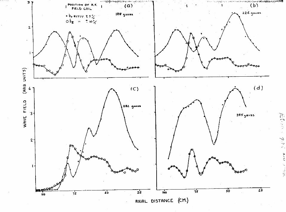
Fig . 7 .1

Graphs of the wave fields br and b Z as a function of axial

distance for an Argon plasma, pressure 1 .5 millitorr . Graphs a, b and c

show the gradually increasing long wavelength component and graph d shows

this wavelength dominant . after the density jump at 380 gauss . A smaller

amplitude short wavelength component can just be seen in graph d .

7 .6

The wavelength impressed on the plasma by the R .F . coil structure

was approximately 50 cm, giving a value of ak = 0 .63 . The wavelength

could not be given a unique. value as it varied along the vessel as can

be seen from figure 7 .1 . In general, the distance between a central pair

of maxima was taken to be a half wavelength . Between I .?(). gauss' and 380

gauss and between 1,90 gauss and 752 gauss, the plasma and wave parameters

changed little . Above 752 gauss, the electron density gradually increased

.with increasing B o to the maximum experimentally attainable of 1500 gauss

with no sudden changes in the plasma or wave parameters . As can be seen,

there is a rapid change in A at 180 gauss and other sudden changesat

3 30 gauss ufJ 751- cj ,:A uss

A difficulty arises in the interpretation of the wavelength measure-

ments since the impressed wavelength is not always the same as the length

of the wave in the plasma . These two modes of oscillation will then inter-

fere making the determination of the plasma wavelength quite difficult .

The wavelengths given in table 7 .1 are therefore only taken to be within

± 50% of the true plasma wavelength .

The measurement of the radial variation of the wave components

proved to be extremely difficult due to perturbation of the plasma by

the probe . After a great number of probes were made and tested, those

shown in figure 6 .1 (numbers 2 and 3) were decided upon . The bent probe

figure 6 .1 (number 4) was used to measure the radial variation of b Z by

rotating the probe about an axis 3 cm from the central axis of the vacuum

vessel . Since this type of probe has a large perturbing effect on the

plasma and pickup by the probe is quite large, b Z was only measured at

very low Bo

30 gauss (figure 7 .2) . The radial measurements of b r and

7 .7

Fig.7 .2

Plot of bZ as a function of radius for low Bo (ti 30 gauss) .

b e were made with short probes inserted radially into the plasma through

one of two side ports . The br probes were of relatively simple construc-

tion with the coil being wound on the outside of a 2 mm piece of pyrex

formed by drawing the end 4 cm of a 20 cm long piece of 6 mm O .D . pyrex

down to 2 mm . This, thin 4 cm of the probe was the only part which entered

the central region of the plasma .

A probe inserted in the other radial port served as a check on the

perturbing effect of the probe making the measurements . If any noticeable

change occurred in the control probe signal as the other was being pushed

in, that set of measurements was discarded .

The be probe utilized a similar piece of pyrex, but the axis of the

probe coil was rotated 900 relative to the axis of the pyrex sheath . The

angular calibration was carried out as described in chapter 6 . Although

this probe could theoretically-measure b z by rotating the probe 900 about

its axis, the b e signal was found to be about an order of magnitude greater

than bz . A slight error in the probe alignment caused large errors in the

wave field and it was decided to measure only b0

. As b 8 has a minimum and

associated phase change between 0 .5 a and 0 .9 a for the m = 1 helicon, this

field component would be sufficient to determine the azimuthal mode, but

the br component was measured radially for the same plasma conditions as

a check . The output of the b 0 and b r probes were calibrated relative to

a constant field of the same frequency (8 .6 MHz) and these normalized

fields are shown as functions of the plasma radius in figures 7 .3 and 7 .4

for a number of axial magnetic fields . As can be seen the wave fields

are representative of the m = 1 helicon over all values of B .0

7 . 8I

7 .9

Mg t 7 .3 .

Plots of br and b6

as functions of radius for a number o

axial magnetic fields .

The b6

component has a 1800 phase change at its minimum value Q 4 3 -

7 .11

7 .3

Langmuir Probes

Initially a floating double Langmuir probe was inserted radially

into the plasma . As the probe had an outside diameter of 6 mm, the

perturbing effects on the plasma column were considerable . A 'bent' probe,

shown in figure 6 .1 (number 1) was then constructed so the probe could be

inserted axially into the plasma and the axial distance at which the radial

measurements of saturation ion current were taken could be varied for

minimum perturbation . This position was generally about 10 cm above the

R .F . coil structure .

Since the probe .. was inserted through a seal 3 cm from the plasma

central axis, the probe could be rotated through all radial positions from

the centre to the wall . The axial magnetic field was varied up to 1200

gauss where the ion Larmor radius was greater than 1 cm assuming an ion

temperature of about 0 .5 eV . For all magnetic fields B 0 'the ion Larmor

radius can be considered to be much larger than the probe electrode

diameter of 0 .1 cm . Therefore, over the greater range of magnetic fields

used in the experiments, the ion saturation current can be considered to

be little effected by the magnetic field . Magnetic fields will, however,

change the ion-collection mechanism . Since the mean-free path of the

electron is of the same order as the length of the vacuum vessel, the

probe can be considered to be collecting ions and electrons from a thin

cylinder of plasma, the length of the column . A measure of the saturated

ion current across a radius will therefore give a reasonably accurate

relative measurement of the charged particle density distribution . The

probe characteristic cannot be interpreted to yield the absolute density

and measurements at different fields cannot be compared to determine

differences in the plasma density,

If the charged particle distribution is Maxwellian, the probe

characteristic can still give the temperature of the electrons for the

lower fields . However, for the high fields (= 1000 gauss), the plasma

may not be isotropic and the plasma should be described by a perpendicular

temperature T1

and a parallel temperature T 11 relative to the field Bo .

The temperature determined from the probe characteristic would therefore

be T // for the high field while the low field determination would give

the isotropic temperature . Figures 7 .5a and 7 .5b show the relationship

between the ion saturation current and radius of the plasma,normalized

to the same central current, while table 7 .3 presents the temperature

deduced from the probe characteristic for a number of different axial

magnetic fields .

The radial variation in the ion saturation current was fitted

with a polynomial using an I .B .M . 1130 computer using a least squares

fitting technique . This approximation, to a typical set of experimental

measurements'is shown in figure 7 .6 . As mentioned previously, the

saturation ion current is directly proportional to the charged particle

density and therefore these radial variations were interpreted as n(r),

the radial density variation, in the computer program describing standing

helicons .

7 .4

Microwave Incerferometer

As the Langmuir probe could not provide an absolute determination

of the plasma density an 8 mm microwave interferometer was used for these

7 . 1 2

I7 .13

Fig .7 .5(a)

Normalized density profiles as a function of radius

determined from Langmuir probe measurements for low magnetic fields .

I7 .14

F4 . 1.5(b)

Normalized density profiles as a function of radius

determined from Langmuir probe measurements for high magnetic fields .

The curves marked 'Iligh' and 'Low' refer to the density jump at 752 gauss .

7 .15

Fig .7 .6

Polynomial fit to measured density profile as a function

of radius . B,=752- cywss )'Low' clenst t y

7 .16

measurements . The average density was 'calculated from the phase shift

measured by the interferometer and the density profile measured with the

Langmuir probe .

The

density across a diameter of the plasma measured by the

interferometer is quite accurate providing the wavelength of the micro-

waves is much smaller than the diameter of the plasma column . In most

modes of operation this was so, but the highly-peaked distribution at

high axial fields would tend to scatter the microwaves . The resultant

phase measurement could only be regarded as a reasonable indication as

to what the true density was . Assuming the microwave beam obeys the laws

of geometric optics, other errors can arise . The main ones are refraction

of the transmitted beam by the plasma and reflection of the beam by the

plasma and by the glass walls of the vacuum vessel . Errors involved in

refraction can be minimized by accurate aligning of the microwave horns

across a diameter of the plasma . This was checked without a plasma by

moving the receiving horn small distances in the axial direction and in

a direction perpendicular to the axis of the horn and maximizing the

transmitted signal .

Reflection of the beam by the glass walls was not negligible as

seen by standing wave maxima and minima when the receiving horn was moved

away from the tube . An estimate of the error associated with these

reflections and those associated with reflection from the plasma was

achieved in the following manner . The frequency of the klystron was

varied by 10% about either side of the frequency used for the measurements

with the plasma between the horns . The density calculated from these

measurements showed a variation of ± 8% . The error involved in the actual

measurement of the density was estimated to be about ±3 degrees of phase

shift which was quite a large error for small densities where the micro-

waves suffered a phase shift of about 20° . For higher densities (> 10 12

electrons/cc) this experimental error decreased to only a few percent as

the phase change increased .

As mentioned above, increasing non-uniformity will introduce large

errors into the interpretation of the phase shift . The magnitude of these

errors are extremely difficult to ascertain as the problem becomes one of

microwave scattering from a thin column of plasma . The density measurements

in these high axial field regions could be up to a factor of two in error .

Table 7 .3 summarizes the variation of density with axial field for a gas

pressure of 1 .5 millitorr . Also included are values of w , 0e, and 0eT,

where T is the time between electron-atom collisions for 3 eV electrons

in Argon (Brown 1959) .

7 .5

Interpretation of Spectroscopic Measurements

Since the'temperatures, densities, and mean-free paths of particles

are different in the large tube and the small tube, the results and dis-

cussion will be presented separately .

Measurements in the Small Tube

A gas pressure of 20 millitorr of Argon was maintained during

these experiments . Measurements taken with 8 mm microwave interferometer

yielded electron densities between 10 11 and 10 13 /cm 3 which varied with

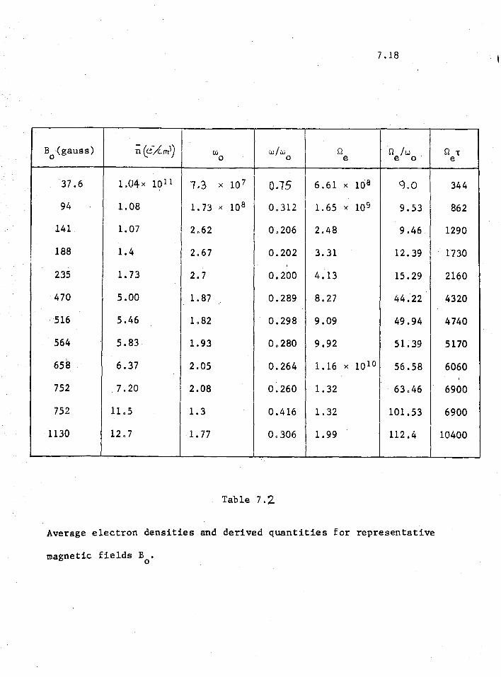
Table 7 .2,

Average electron densities and derived quantities for representative

magnetic fields Bo .

B0 (gauss) n(e/MI) wo 0 Q -r

37 .6

94

141

188

235

470

516

564

658

752

752

1130

1 .04x 10 11

1 .08

1 .07

1 .4

1 .73

5 .00

5 .46

5 .83

6 .37

7 .20

11 .5

12 .7

7 .3 x 10'

1 .73 x 108

2 .62

2 .67

2 .7

1 .87

1,82

1 .93

2 .05

2 .08

1 .3

1 .77

0 .75

0 .312

0,206

0 .202

0 .200

0 .289

0 .298

0 .280

0 .264

0 .260

0 .416

0 .306

6 .61 x 108

1 .65 x 109

2 .48

3 .31

4 .13

8 .27

9 .09

9 .92

1 .16 x 10 10

1 1 .32

1 .32

1 .99

9 ..0

9 .53

9 .46

12 .39

15 .29

44 .22

49 .94

51 .39

56.58

63 .46

101 .53

112 .4

344

862

1290

1730

2160

4320

4740

5170

6060

6900

6900

10400

7 .18

7 .19

B0 in a similar manner to that described in section 1 of this chapter, The

Doppler broadening measurements on the Ha line yielded an ion temperature

of 6000 ± 2000°K over all values of B° and consequently over all values of

density , measured . The relative intensities of eleven Argon II lines were

measured and the electron temperature so deduced was 12,000 ± 2400°K . In

one experiment Hydrogen was used as a trace gas in Argon at a pressure of

20 millitorr . The relative intensities of the Argon II lines yielded the

Same temperature as mentioned above, but the relative intensities of the

Balmer lines of Hydrogen showed a large deviation from L .T .E . (figure 7 .7) .

As mentioned in chapter 6, section 4, quantum states can be considered to

be in quasi L .T .E . if they lie close together and close to the ionization

potential . It can be seen from figure 7 .7 that the graph of the intensities

is approaching an asymptote for the higher energy levels . This asymptote

represents an electron temperature of 1300°K .

In the case of Hydrogen, atomic transitions were being observed and

since the plasma density was highly peaked in the centre of the tube, the

neutral density was a maximum at the walls where the electron temperature

would be quite low (Cross, James and Watson-Munro 1969) . The greater part of

the light measured would arise from these neutrals, resulting in the low

electron temperature measurement .

Langmuir double probe

measurements gave an electron temperature

of 18,000 + 2,000 °K or approximately 50% greater than that deduced from

the Argon II lines . This discrepancy is probably due to the fact that the

plasma density was too low to assume L .T .E . and the excitation mechanism

for electrons in the Argon II lines is not a simple collisional phenomena .

The de-excitation coefficient X(T e, p, q) is not known accurately at

present for low density plasmas and could introduce large errors into the

7 . 2 0

Fig . 7 .7

Plot of the relative intensities of a number of Balmer lines

against the energy of the transition . For the small tube with 20 millitorr

of Argon and a trace of hydrogen, RF = 8 .6 MHz .

7 .21

temperature measurements . The R .F . fields may also produce an incorrect

temperature in the Langmuir probe measurements .

The high energy group of electrons reported by Schluter was not

observed in the plasma . However, if the density of this group of electrons

was very low it is unlikely that they would affect significantly the

intensity distribution of the Argon II lines, or the shape of the Langmuir

probe characteristic .

As the measurements in the small tube were made mainly to test

different diagnostic methods, no further measurements were carried out,

and temperature determination in the large tube was restricted to Langmui .r

.probe and Argon II line intensity measurements .

Measurements in the Large Tube

Although the line densities in this apparatus were similar to those

in the small apparatus, the neutral gas pressure was about an order of

magnitude lower and was generally kept at 1 .5 millitorr . Consequently,

the mean-free path of the electrons was considerably greater than in the

Small tube and was greater than the length of the vacuum vessel . Relative

line intensities of thirteen Argon II lines were measured and a log-linear

plot of the intensity against excitation energy yielded a temperature of

3 .2 x 104 OK with an error of ± 10% . The line of best fit to the experi-

mental points was determined by using a least squares analysis on an I .B .M .

1130 computer .

Electron temperatures were also deduced from Langmuir double probe

measurements taken at a fixed position on the central axis of the tube .

Table 7 . 2

Errors involved in the experimental measurements using the probe

were ± 7% at most .

The average temperature can be seen to be approximately 3 eV,

agreeing well with the temperature measured spectroscopically . The

temperature deduced from the probe measurements assumes only that the

electrons have a Maxwellian distribution of energies, The temperature

deduced from the spectroscopic measurements assumes that the levels

involved in the transitions are in local thermodynamic equilibrium (L .T .E .)

7 .22

The temperatures so deduced are set out in the table below .

B0 (gauss) Te ( 0K)

37,6

141

235

29,000

33,000

32,000

I

470 28,000

516 30,000

564 27,000

658 35,000

752 33,000

752 37,000

7 .23

with each other and with the free electrons, which are assumed to have a

Maxwellian distribution . Although the electron densities (ti 1012/ cc) are

too low to invoke the L .T .E . model, the agreement between these two methods

which involve different assumptions implies that the temperature so meas-

ured is that of the majority of the electrons . The possibility of the

existance of a much higher energy group of electrons is not discounted .

By analogy with the measurements taken on the smaller apparatus, a high-

energy group of electrons would be expected and the damping of the helicon

wave (discussed below) can be explained by the existance of these electrons .

7 .6

Discussion

For clarity of presentation, this final section is divided into two

parts . The first part will deal with the bulk properties of the plasma

formed by the interaction of the R .F . fields with the Argon . The second

part will consist of a discussion of the interaction between the helicon

wave and the charged particles constituting the plasma .

Bulk Propertiesofthe Plasma

It has been shown in the previous sections of this chapter that

an Argon plasma in a magnetic field with an average density of 2 x 10 12

charged particles/cm3 over a volume of 7,500 cm3 can be achieved with

low power (< 200 watts) radio-frequency power . The gas pressure was 1 .5

millitorr representing a neutral density of 5 k- 10' 3 atoms/cm 3 . The

percentage ionization was therefore 4% over the volume occupied by the

plasma . Since the plasma was highly non-uniform, the density at the

7 . 24

central axis was a factor of four greater than the average, representing

a percentage ionization of 16% . The plasma could be run continuously or

in a pulsed mode .

Wavelength and Density Measurements

Before the detailed measurement's of wavelength and density were

taken, a number of runs were carried out for pressures ranging from 0 .5

to 5 .0 millitorr of Argon . It was found that the maximum plasma densities

were achieved at about 1 .5 millitorr . Above and below this pressure the

large density jumps (b and c in figure 7 .8) did not occur and the measured

wavelength remained approximately the same as the impressed wavelength .

The density increased proportionally with B0

so that w/wo remained

approximately constant as would be expected from the simple theory of

Helicons . The most interesting phenomena occured at 1 .5 millitorr where

the strong interaction between the wave fields and the plasma appeared as

large jumps in density and wavelength . The detailed measurements described

in this chapter were therefore restricted to this pressure . Although

there is no adequate theory at present, the dispersion of the wave can be

described qualitatively by referring to the simple plane wave theory

(W/W0 a k2) and to the effect of radial density non-uniformity (Christiansen

(1969)) .

For fields of a few tens of gauss, the wave did not couple well

into the plasma but as B0increased to 180 gauss, the wave fields became well

formed and the dispersion can be described by the plane wave theory with

a small degree of non-uniformity which gives a rather shorter wavelength

than would be expected . At 180 gauss, the density increased by a factor

of 1 .4 and the wavelength decreased by a factor of 1 .3, in reasonable

agreement with theory . Between 180 and 380 gauss the wavelength decreased

slightly while the density and non-uniformity increased, again in general

t

7 . 2 5

agreement with theory . However, as can be seen from figure 7 .1 a, b and

c, the wave fields became progressively more distorted . The'large density

jump at 380 gauss and the large increase in wavelength cannot be explained

by the simple theory of Helicons . This can be explained qualitatively

if the the wave is considered to be within a cavity about 100 cm long defined

by the axial magnetic field . In general, the simplest mode of a cavity will

be least damped, with more complicated modes suffering progressively

greater attenuation . The distortion noted in figure 7 .1 a, b and c, was

probably due to mode competition between the wavelength impressed by the

R .F . coil and the much longer wavelength defined by the cavity . As Bo

increased from 188 gauss, the cavity mode gradually increased in amplitude

until at 380 gauss it suddenly became the dominant wavelength (Figure 7 .1 d) .

This change had an associated rapid increase in density implying that the

cavityy mode interacted strongly with the plasma .

The dispersion of the wave from 380 gauss to 752 gauss can be

described by gradually increasing density and non-uniformity . At 752 gauss,

the density increased by a factor of 1 .6 and the wavelength decreased by a

factor of 1 .2 in good agreement with theory . For Bo greater than 752 gauss,

the density and non-uniformity gradually increased with B o with little

resulting change in the measured wavelength .

As Boincreased, the wave fields became more peaked in the centre

of the tube (figures 7 .3, 7 .4) . The br and be components became far larger

than b z causing the energy dissipation of the wave (t1j 2 ) to become more

concentrated in the centre of the tube (section 3 .3) . This would appear

as an increase in the radial density non-uniformity, as can be seen in

figure 7 .5 a and b .

Although the density increased by an order of magnitude as B o

increased, the R .F . power being fed into the R .F . coil increased by only 10% .

7 .26

This discrepancy was presumably due to power radiated into the laboratory

at lowBo

rather than being absorbed in the plasma .

Although' the standing Helicon wave described in this chapter is of

quite low amplitude (b/Bb 4 1%) the sudden density jumps and changes in

wavelength implied a strong interaction existed between the wave and the

plasma . At present no theory exists which can adequately describe the

dispersion and attenuation characteristics of the system described above .

The most comprehensive theoretical model for the dispersion of Helicon waves

in a non-uniform plasma that has been developed at this time is given in

section 3 .5 . As mentioned in section 4 .2, it adequately describes the

dispersion and attenuation of small amplitude Helicons in collision

dominated plasmas (pressures of 10 - 70 millitorr in the case of Lehane and

Thonemann (1965)) .

The experiments described in this chapter were carried out at a

pressure of 1 .5 millitorr where the electron mean free path was quite

large (greater than 30 cm) and the wave attenuation would be dominated by

non-linear effects such as wave-particle interactions and ionization . It

is reasonable to assume that these effects will manifest themselves

throughout the volume of the plasma and therefore a damping parameter can

be assigned to the interaction . Any difference between the theoretical

value of the damping parameter Qe T (where T is calculated from the cross

section for momentum transfer) and the value required to fit the experi-

mentally measured wave fields would give an indication of the magnitude

of the non-linear attenuation of the wave . The theory given in section

3 .5 was used with the assumption that S2 eT was a fitted parameter covering

all forms of volume damping .

Fig . 7 .8

Sketch of electron density as a function of ho for 1 .5 milli-

torr of Argon (derived from table 7 .2) .

7 . 2 7

7 .28

As we are dealing with a standing wave, the angular frequency has

an imaginary part (w=wr+iwi) which describes the damping of the wave in

time . The experimentally determined values of the parameters are given

in table 7 .3 . The polynomial approximation to the radial density profile

for each value of Bo was also inserted into the program. A collision fre-

quncy appropriate to 3 eV electrons in 1 .5 millitorr of Argon was used in

determining 0e T . As the values of 0eT are very large, an extremely low

damping would be expected . The anamolous damping postulated by K.M.T . was

shown in chapter 4 to be non-existant when electron inertia was included .

Computation of the dispersion relation for these high values of 0eT

produced wave fields with a radial variation greatly different from the

experimentally measured variation . Since the experimentally measured wave

fields were considered to be the most reliable measurements of the wave

characteristics, the value of 0T was varied to make the radial positione

of the phase change in b e coincide with the experimental measurement

(figure 7 .9 a,b) . Two values of the wavelength were chosen to be double

the

length of the exciting coil (ak = 0,63) and four times the

length of the exciting coil (ak = 0 .31) . The real part of the wave

frequency is fixed by the R .F . oscillator frequency . Sets of curves were

computed for these two values of ak for differing values of QeT (figure

7 .10) .

Numerical errors in computing solutions for Bo > 800 gauss were

considerable due to the high degree of radial density non-uniformity and

the last two experimental points were not considered theoretically . It

can be seen from figure 7 .10 that for fields between 450 gauss and 750

gauss, the experimental results can be described by a standing helicon

7 .29

Fib 7 .9 (a te)

'Theoretical curves for two different values of r2 T inc

an attempt to fit the experimentally measured b r and b0 profiles . Argon

at 1 .5 Millitorr, Bo = 37 gauss, RF = 8 .6 MHz, fitted value of ak = 0 .63 .

0

0

Experimental points

S2T =3e

Z T = 300 .

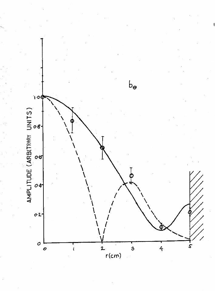
Fig . 7 .10

Theoretical fitting of solutions for a number of values of

SZ -r and ak .e

W (D

Theoretical curves .

Experimental points .

7 .30

7 .31

wave in a cold plasma with ak ti 0 .6 and 3 < 0eT < 4 . Experimental points

for magnetic fields less than 450 gauss are not well described by these

values of ak and 0eT . If the experimental values of ak in this region are

used (ak % 1) the theoretical values diverge further from the experimental

values . The increase in w/wo at Bo = 750 gauss has an associated increase

in the wave number which is in qualitative agreement with the linear theory .

In the region 450 gauss < Bo < 750 gauss, the value of 0eT from

table 7 .3 yields a damping factor due to electron-atom collisions :

wi

' 10-3wr toll

To estimate the damping due to Cherenkov mechanism in cylindrical geometry,

the formula derived by Dolgopolov (1963) is used :

wi ti ki kvTwr

kr

Qe

ti k? + k2 /''T

Pe

To estimate k1, the perpendicular wave number, we assume .a uniform plasma

with conducting boundaries,with the boundary condition, b r = 0

i .e . J1(kja) = 0

kla = 3 .8

kZ ti 0 .76 cm -1 .

7 .32

Assuming ak// = 0 .63, then k// u 0 .13 ,

therefore wi`

8 x 10-3 ,wr cher

(since for 3 eV electrons, the thermal speed (VT) is ti 108 cm/sec) .

The Cherenkov mechanism is about an order of magnitude greater than

the collisional damping mechanism, but is still far less than damping for a

fitted value of Q T - 3 :e

witi 4 .

Wr fit

Although there is a large difference in the damping due to the Cherenkov

mechanism and the 'fitted' damping, the electrons contributing to the

damping in the model proposed by Dolgopolov are assumed to obey a Maxwellian

distribution . This assumption has been shown to be invalid for low density

(10 13 electrons/cm 3) R .F . maintained plasmas earlier in this chapter .

Another complication arises from the basic property of helicon

waves that the electrons are tied to the lines of force of the wave .

Since w << 0e the electrons will move with the moving field lines with

a small cycloidal motion. The electron temperature will be anisotropic

and will be a function of r, 6, and z, i .e . vT(r,6,z) .

In sections 5 and 6 of this chapter the electron temperature meas-

ured by an axial Langmuir probe is discussed . It was shown that this

temperature can only be taken to represent the z-component . Since this

temperature was constant for all values of the magnetic field Bo it would

seem to be a good estimate of the parallel component . The electrons moving

radially would have a number of collisions with the walls in the distance

7 .33

of a mean-free path and would not gain a significant amount of energy from

the wave .

Electrons moving in the azimuthal direction can continuously absorb

energy from the wave and would be reflected by the "magnetic mirrors" of

the standing helicon field . As the z-component of the velocity remains

constant for all Bo, the electrons moving in the d direction would be

trapped in the magnetic field of the wave and would acquire energy from

the helically moving wave fields . A high-energy group of electrons is

required to keep the plasma in a stationary state and they must gain their

energy from the wave fields . Qualitatively it can be seen that these

electrons will have a considerable effect on the damping of the wave since

in the collisionless mechanism the damping of the wave is proportional to

the number of electrons absorbing energy .

The investigations described in this, thesis have shown that the

linear theory, including the effects of electron inertia and radial

density non-uniformity, for the propagation and attenuation of a standing

helicon wave is inadequate to describe the wave discussed above . The

effects on the wave of conducting and non-conducting boundaries have been

investigated and the case of low resistivity for a wave in a plasma with

non-conducting boundaries has been examined in some depth . Although the

real part of the frequency predicted by the linear theory was only a

factor of 2 or' 3 away from the measured value, the dampin g wwas about

r,

four orders of magnitude smaller than the measured value . To explain this

large difference, it was shown above that the inclusion of thermal effects

can increase the damping by an order of magnitude over the linear theory,

but is still far less than expected experimentally .

7 .34

To formally solve this problem, a full theoretical analysis

involving the calculation of anisotropic thermal effects on the wave

dispersion and attenuation with the Boltzmann equation is required .

7 .7

Possible Studies Arising from this Work

The study of instabilities is of considerable interest in working

toward controlled thermonuclear reactions . The anomalous high resistivity

in the Tokomak machines is thought to be due to the presence of instab-

ilities arising from particle wave interactions . Since the helicon wave

can be heavily damped due to the Cherenkov mechanism, this study indicates

that the suggestions outlined below may be of of interest .

(1)

A theoretical analysis of anisotropic thermal effects on a wave

propagating within a cylindrical plasma .

(2)

Injecting beams of electrons parallel to the axis of the plasma

to examine the Doppler shifted cyclotron absorption .

(3) Injecting beams of electrons at the same angle as the lines of

force of the helicon wave to confirm the qualitative results of

this thesis .

(4)

Wave echo experiments to validate the assumption of a collisionless

plasma and to investigate the echo phenomena .

(5)

Propagating waves near the

cyclotron frequency to investigate

the collisionless cyclotron damping mechanism .