CHAPTER 7OPTIMAL LOCATION OFISOLATION VALVES IN WATERDISTRIBUTION SYSTEMS:A RELIABILITY/OPTIMIZATIONAPPROACH

Sukru OzgerCarollo EngineersPhoenix, Arizona

Larry W. MaysDepartment of Civil and Environmental EngineeringArizona State UniversityTempe, Arizona

7.1 INTRODUCTION

7.1.1 Before September 11, 2001

The cornerstone of any healthy population is access to safe drinking water. The goal of the UnitedNations International Drinking Water Supply and Sanitation Decade from 1981 to 1990 was safedrinking water for all. A substantial effort was made by the United Nations to provide drinking waterand sanitation services to populations lacking those services. Unfortunately, however, the growth indeveloping country populations almost entirely wiped out the gains. In fact nearly as many peoplelack those services today as at the beginning of the 1980s (Gleick, 1993, 1998).

The lack of adequate water supply systems is due to both the deterioration of aging water sup-plies in older urbanized areas, and to the nonexistence of water supply systems in many areas thatare undergoing rapid urbanization, such as in the southwestern United States. In other words, methodsfor evaluation of the nation’s water supply services needs to consider not only rehabilitation of exist-ing urban water supply systems but also the future development of new water supply systems to serveexpanding population centers. Both the adaptation of existing technologies and the development of newinnovative technologies will be required to improve the efficiency and cost-effectiveness of futureand existing water supply systems and facilities necessary for industrial growth.

An EPA survey (Clark et al., 1982) of previous water supply projects concluded that the distri-bution facilities in water supply systems account for the largest cost item in future maintenancebudgets. The aging deteriorating systems in many areas raise tremendous maintenance decision-making problems that are further complicated by the expansion of existing systems. Deterioration ofthe water distribution systems in many areas has translated into a high proportion of unaccounted-forwater due to leakage, which is not only a loss of a valuable resource, but also raises concerns of safedrinking water by possible contamination through cracked pipes.

The reliability of the existing aging systems is continually decreasing. Only recently have manymunicipalities been willing or able to finance rehabilitation of deteriorating pipelines, and are stilldeferring needed maintenance and replacement of systems components until a catastrophe or themagnitude of leakage justifies the expense of repair. Water main failures have been extensive in manycities.

7.1

Ch07_Mays_144381-9 9/28/04 12:01 AM Page 7.1

As a result of governmental regulations and consumer-oriented expectations, a major concernnow is the transport and fate of dissolved substances in water distribution systems. The passage ofthe Safe Drinking Water Act in 1974 and its amendments in 1986 (SDWAA) changed the manner inwhich water is treated and delivered in the United States. The U.S. Environmental Protection Agency(USEPA) is required to establish maximum contaminant level (MCL) goals for each contaminantthat may have an adverse effect on people’s health. These goals are set to the values at which noknown or expected adverse effects on health can occur. By allowing a margin of safety (Clark et al.,1987; Clark, 1987) previous regulatory concerns were focused on water as it leaves the treatment plantbefore entering the distribution system (Clark, 1987), disregarding the variations in water quality thatoccur in the water distribution systems.

7.1.2 After September 11, 2001

Water utilities are implemented to construct, operate, and maintain water supply systems. In the pastthe basic function of these water utilities was to obtain water from a source, treat the water to anacceptable quality, and deliver the desired quantity of water at the desired time. The events ofSeptember 11, 2001 and subsequent anthrax attacks have shown the vulnerability of basic civilianinfrastructure, somewhat changing the function of water utilities to include protection from variousthreats. Drinking water supply systems around the world offer great opportunities for terrorism asthese systems are extensive, relatively unprotected and accessible, and often isolated. The threats tothese systems include cyber, physical, chemical, and biological threats.

The events of September 11, 2001 have significantly changed the approach to management ofwater utilities. Previously the consideration of terrorist threats to our nation’s drinking water supplywas minimal. New trends in the technical management of water supply systems will be heavilyfocused upon security issues as related to the design, operation, and management of these systems.Of particular interest will be the evaluation of risk and reliability issues of the various components,the subsystems, and the systems as a whole from the viewpoint of their susceptibility to terrorism.

Within a very short time after September 11, 2001 we began to see a concerted effort at all levelsof government to begin addressing issues related to the threat of terrorist activities to the U.S. watersupply. We saw a number of acts passed such as the “Security and Bioterrorism Preparedness andResponse Act” and the “Homeland Security Act” that addressed the nation’s water supply. These actsresulted in agencies such as the U.S. Environmental Protection Agency (EPA) developing new pro-tocols to address their new responsibilities under these acts.

7.1.3 Water Distribution Systems: A Brief Description

Water distribution systems are composed of three major components: pumping stations, distributionstorage, and distribution piping. These components may be further divided into subcomponents,which in turn can be divided into subsubcomponents. For example, the pumping station componentconsists of structural, electrical, piping, and pumping unit subcomponents. The pumping unit can bedivided further into subsubcomponents: pump, driver, controls, and power transmission. The exactdefinition of components, subcomponents, and subsubcomponents depends on the level of detail ofthe required analysis and to a somewhat greater extent on the level of detail of available data. In fact,the concept of component-subcomponent- subsubcomponent merely defines a hierarchy of buildingblocks used to construct the water distribution system.

A water distribution system operates as a system of independent components. The hydraulics ofeach component is relatively straightforward; however, these components depend directly upon eachother and as a result affect each other’s performance. The purpose of design and analysis is to deter-mine how the systems perform hydraulically under various demands and operating conditions. Theseanalyses are used for the following situations:

� Design of a new distribution system� Modification and expansion of an existing system

7.2 CHAPTER SEVEN

Ch07_Mays_144381-9 9/28/04 12:01 AM Page 7.2

� Analysis of system malfunction such as pipe breaks, leakage, valve failure, and pump failure� Evaluation of system reliability� Preparation for maintenance� System performance and operation optimization

Books on the subject of water supply/water distribution systems include Mays (1989, 2000, 2002,2004a). The subject of security of these systems is covered in detail in Water Supply Security Systemsby Mays (2004b).

Distribution systems, consisting of pipelines, pipes, pumps, storage tanks, and the appurtenancessuch as various types of valves, meters, and the like, offer the greatest opportunity for terrorismbecause they are extensive, relatively unprotected and accessible, and often isolated. The physicaldestruction of a water distribution system’s assets or the disruption of the water supply could be morelikely than contamination. A likely avenue for such an act of terrorism is a bomb, carried by car ortruck, similar to recent events. Truck or car bombs require less preparation, skill, or manpower thancomplex attacks such as those of September 11, 2001. However, we must consider all possiblethreats no matter how remote we may think that they could be.

7.2 DEMAND-DRIVEN ANALYSIS VERSUS PRESSURE-DRIVENANALYSIS

7.2.1 Definitions

Hydraulics of a water distribution network can be approached from two different perspectives. Thedifference between them comes from the level of primacy given to nodal demands vs. nodal pres-sures. The first approach assumes that consumer demands are always satisfied regardless of the pres-sures throughout the system and formulates the constitutive equations accordingly to solve for theunknown nodal heads. This approach is called demand-driven analysis and is used by almost all thetraditional network hydraulic solvers. Examples are EPANET by Rossman (1994) and KYPIPE byWood (1980).

A water distribution network can be designed or operated using demand-driven analysis undernormal operating conditions. This is usually done by adjusting such independent decision variablesas simple or rule-based controls for pump operations, valve settings, reservoir/tank levels, and so on.If a proper design has been made for a given design demand loading, then nodal pressures through-out the system should be well above the minimum pressure required. On the other hand, if the samenetwork were analyzed with a higher demand loading, it would not be surprising to see warning mes-sages such as “Negative pressures at 6:00 hrs” from the EPANET model while nodal demands arefully satisfied at the same time period. Almost all demand-driven models possess a partial recogni-tion of this weakness with similar warning messages when negative pressures are calculated from anetwork hydraulic analysis.

The major drawback of the demand-driven approach is that it fails to measure a partially failednetwork performance resulting from abnormalities in physical and nonphysical system components(e.g., pipe breaks, fire-fighting demands, etc.). In such cases, if demand-driven analysis is used, itmay produce very unrealistic results; for example, negative pressures are calculated at some nodesin the system. It is not uncommon that a hydraulic analysis using a demand-driven approach yieldslarge negative pressures at one or more junctions of a distribution network.

The second approach to a network hydraulic analysis is called head-driven (occasionally calledpressure-driven or pressure-dependent) analysis. Here, the primacy is given to pressures. A node issupplied its full demand only if a minimum required supply pressure is satisfied at that node. If theminimum pressure requirement cannot be met, then only a fraction of the nodal demand can be satis-fied. That fraction is determined by a predefined relationship between nodal head and nodal outflow.

As mentioned above, demand-driven models work well under normal operating conditions.Major applications of head-driven analysis, on the other hand, are for analysis of network perfor-mance under partially failed conditions. Because a network reliability assessment requires evalua-

OPTIMAL LOCATION OF ISOLATION VALVES 7.3

Ch07_Mays_144381-9 9/28/04 12:01 AM Page 7.3

tion of partially failed conditions of a network, pressure-dependent analysis is much more suitablefor reliability assessment of water distribution networks.

One of the major problems with the pressure-driven approach is that it requires extensive fielddata collection to determine the relationship between nodal heads and nodal flows. Such a relation-ship may be unique for each junction of a network inasmuch as it depends on such physical charac-teristics as type of service connection and the development type that the junction serves (e.g.,residential, high-rise, schools, hospitals, etc.). Calibration of models using field data is also part ofthe extensive effort needed to be able to use pressure-dependent analysis.

The second major drawback of head-driven analysis is that it lacks robust methods for the com-putational solution of the constitutive equations (Tanyimboh et al., 2001). Almost all the traditionalnetwork hydraulic models are built upon the demand-driven approach. Therefore, it is very desirablethat reliability analysis techniques based on interpretations or transformations of existing demand-driven analysis from a pressure-driven approach be developed.

7.2.2 Hydraulic Equations for a Network Simulation Problem

Two sets of equations are needed to solve a network simulation problem. First, conservation of flowmust be satisfied at each network junction. The second set of equations describes a nonlinear rela-tion between flow and headloss in each pipe, such as the Hazen-Williams or Darcy-Weisbach equation.These equations form a coupled set of nonlinear equations whenever the network contains loops ormore than one fixed-head source (Rossman, 2000). The fact that most distribution systems arelooped and/or have multiple sources requires the aid of a computer to solve the nonlinear set of equa-tions using an iterative procedure. The basic equations in a network model are described by Rossman(2000) for a network with N junction nodes and NF fixed grade nodes (tanks and reservoirs).

Let the flow-headloss relation in a pipe between nodes i and j be given as:

Hi � Hj � hij � rQifn � mQif

2 (7.1)

where H � nodal headh � headlossr � resistance coefficient

Q � flow raten � flow exponent

m � minor loss coefficient

The value of the resistance coefficient and the corresponding flow exponent depend on which fric-tion headloss formula is being used. Most network models use one of the following flow-headlossrelationships: (1) Hazen-Williams, (2) Darcy-Weisbach, or (3) Chezy-Manning.

In addition to the first set of equations described above, conservation of flow around all nodesmust be satisfied, which forms the second set of equations

�j

Qif � Di � 0 for i � 1,…,N (7.2)

where Di � flow demand (or supply) at node ij � set of nodes directly connected to node i

Qij � flow in pipe ij

By convention, flow is positive if it is into the subject node and negative, otherwise.As previously mentioned the conventional network hydraulic solvers such as EPANET by

Rossman (1994) and KYPIPE by Wood (1980) are demand-driven. Demand-driven analysis seeks asolution for all heads Hi and flows Qij that satisfy the two sets of equations, (7.1) and (7.2), for a setof known heads at the fixed grade nodes. The basic assumption in demand-driven analysis is thatnodes are assigned demands that are assumed fully satisfied. For example, variables used in the solu-tion algorithm of EPANET are divided into unknown and known variables (Rossman, 1994).

7.4 CHAPTER SEVEN

Ch07_Mays_144381-9 9/28/04 12:01 AM Page 7.4

The unknown variables are

ys � height of water stored at tank node s

Qs � flow into storage tank node s

Qij � flow in pipe connecting nodes i and j

Hi � hydraulic grade line elevation at node i (elevation plus pressure head)

and the known variables (constants) are:

As � tank cross-section area

Es � elevation of node s

Di � demand (or supply) at node i

The major assumption of demand-driven analysis, that demands are fully satisfied, works wellunder normal operating conditions. However, it is not uncommon that under abnormal conditions asolution arises where pressures are negative or unacceptably low, because demands are satisfiedregardless of validity of calculated pressures at network nodes (Bouchart and Goulter, 2000). A fewexamples of such abnormal conditions may occur when demand loading on the network exceeds thedesign demand loading, fire-fighting demands for which the network was not designed, or closure ofa portion of a network because of contamination or pipe main breaks. In reality, a shortfall in the vol-ume of water actually delivered to consumers begins as the pressure in the network drops below somethreshold value. Naturally and ideally, a lower bound for this threshold value is zero gauge pressure.

Water distribution networks are almost always skeletonized to some degree, depending on themodeling purpose forcing demands from secondary networks to be lumped into nearby junctions.Because of various headlosses associated with secondary networks and different elevations of outletsin these networks, it is very difficult, if not impossible, to define a relationship between the pressureat a junction and the flow available from that junction into the secondary network it serves. A tediousway of doing this is field data collection and calibration. A typical value for threshold pressure isbelow the minimum of 20 m in network studies (Bouchart and Goulter, 2000). Tanyimboh et al.(1999) state that pressures of 15 to 25 m are the minimum acceptable standards with the use of net-work models. All this implies that demand-driven algorithms cannot cope with situations where pres-sures are less than satisfactory at some demand nodes (Tanyimboh et al., 2001) and thus fail to depictdeficient network performances.

7.2.3 Service Pressures

Criteria for assessing acceptable service pressures in a distribution network may vary from systemto system. Therefore, there are no universally acceptable pressure ranges. Chin (2000) lists the fol-lowing considerations for assessing the adequacy of service pressures:

1. Flow is adequate for residential areas when pressures are above 240 kPa (35 psi);

2. The pressure required at street level for excellent flow to a 3-story building is about 290 kPa (42 psi);

3. Adequate flow to a 20-story building would require about 830 kPa (120 psi) of service pressureat street level, which is not desirable because of the associated leakage and waste. Thus, very tallbuildings are usually served with their own pumping system;

4. In general, pressures in the range of 410 to 520 kPa (60 to 75 psi) would be adequate for

� Supplying normal water delivery to buildings up to 10 stories� Providing adequate sprinkler service in buildings of 4 to 5 stories� Supplying water for fire protection� Handling fluctuations in pressure caused by clogged pipes and excessive length of service

pipes.

OPTIMAL LOCATION OF ISOLATION VALVES 7.5

Ch07_Mays_144381-9 9/28/04 12:01 AM Page 7.5

Overall, pressures in most cases should be maintained above 207 kPa (30 psi) and below 689 kPa(100 psi) during normal operations. Pressures above 689 kPa tend to increase water waste through unde-tected leaks and may cause damage to residential and commercial plumbing systems or pipe breaks. Theminimum pressure requirement may be lowered to 138 kPa (20 psi) during emergency conditions, suchas a fire. A 138 kPa pressure is sufficient to supply the suction side of pumps on a fire pumper truck.According to Walski (2000), the threshold pressure value below which a failure to satisfy the fulldemands occurs is usually assumed to be below the minimum of 20 m (�196 kPa or 28.4 psi).

The Office of Water Services in England specifies a minimum acceptable static pressure of 7 m(�68.5 kPa or 10 psi) below which customers may be entitled to compensation for less than satis-factory service. On the other hand, it is not uncommon that minimum acceptable pressure is specifiedas high as 25 m (�245 kPa or 35 psi), to allow for possible increases in demand (Tanyimboh et al.,1999). In general, nodal pressures of 15 to 25 m will guarantee satisfactory service at all related stoptaps in a distribution system. Pressures that are lower may cause a shortfall in supply and failure tosupply the full demands. Tanyimboh et al. (1999) also suggest that in the absence of field test data,a good approximation to critical pressures can be obtained by the equivalent static pressure to theheight above ground level of rooftop water tanks in typical two-story residential areas.

Water-using devices in residential houses may also require certain minimum pressures to operate.For example, most dishwasher manufacturers specify minimum working pressures anywhere from20 to 40 psi.

Another factor that should be considered while estimating the critical pressure is the degree ofnetwork skeletonization. Typically, smaller pipes in a network are excluded from the modeling. Theresult is that total demand from the consumers located along those smaller lines is lumped intothe nearby junctions located on larger pipes. Thus, when choosing the critical pressure for a junc-tion, such characteristics as outlet elevations and headlosses of the secondary network that the junctionserves must also be taken into account.

7.2.4 Head-Driven Analysis

Demand-driven analysis explained in the previous section assumes that consumer demands in a dis-tribution network are fully satisfied regardless of validity of calculated pressures. It can be arguedthat many modern water-using devices such as toilets, washing machines, and dishwashers are essen-tially pressure-independent provided a minimum threshold pressure is available, which supports theassumption of primacy of demands.

The philosophical basis of head-driven analysis—the counterapproach to demand-driven analysis—is explained by Rossman (2001) as follows.

…[A] distribution system can be thought of as a completely closed, pressurized system witha set of variable sized orifices that connect to various devices that are open to the atmosphere(e.g., sinks, toilets, water heaters, washing machines, pipe leaks, etc.). For a specified opening ofthese orifices, the flow out of them will be dependent on the pressure maintained in the system(which in turn is dependent on the setting of the demand orifices).…

Thus, unlike demand-driven analysis, the head-driven approach treats demands as random vari-ables and recognizes the primacy of pressures by defining a relationship between the outflow and thepressure at each node. This relationship is given, in its general form, by (Tanyimboh et al., 1999)

Hj � Hjmin � KjQj

nj (7.3)

where Hj � head at node j corresponding to demand QjKj � flow resistance coefficientnj � exponent

Hjmin � minimum required nodal head below which outflow at node j is unsatisfactory or zero

Because demands are unknown, Eq. (7.3) can be rearranged:

7.6 CHAPTER SEVEN

Ch07_Mays_144381-9 9/28/04 12:01 AM Page 7.6

Qj � � �1/nj

(7.4)

The head-driven analysis requires substitution of Qj into Eq. (7.2) in the place of Di. The solutionalgorithms for solving the resulting problem have been described by Gupta and Bhave (1996) andTabesh (1998).

As explained in the previous section, demand-driven analysis may produce unrealistic results(i.e., pressures being negative or less than satisfactory) especially under partially failed conditions ofa system. In such cases, head-driven analysis is superior to the demand-driven approach in that theformer is able to determine the nodes with insufficient supply and the respective magnitudes ofthe shortfalls. On the other hand, performing a head-driven analysis requires extensive field data col-lection and calibration to determine K and n values, possibly for each node (Gupta and Bhave, 1997).In addition to these practical difficulties, lack of robust methods for computational solution of con-stitutive equations in head-driven analysis makes the demand-driven network models the primarychoice for hydraulic analysis or reliability assessments.

7.2.5 Node Flow Analysis

In order to overcome the weaknesses of demand-driven analysis, Bhave (1991) developed a methodcalled Node Flow Analysis (NFA) to predict performance when a distribution network is deficient.The method was based on the assumption that when a network is deficient and thus unable to satis-fy the nodal demands, the network will try to meet the demands, as far as possible, under the givenconditions. In other words, the flow in the network will adjust such that the total supply is maximizedunder deficient conditions. Thus, the network flow analysis problem is considered as an optimiza-tion problem in their node flow analysis subject to certain constraints that relate hydraulic gradelineat each junction to available flow at that junction.

The complete optimization problem is as follows:

� �j

qj (7.5a)

where qj is the flow available at node jSubject to:

Hm � Hom for all m (7.5b)

where m is number of source nodes and Hom is the specified hydraulic grade line (HGL) value atsource node m.

qj � qjreq if Hj � Hj

min (7.5c)

or

0 � qj � qjreq if Hj � Hj

min (7.5d)

or

qj � 0 if Hj � Hjmin (7.5e)

�i

Qij � qj � 0 for all j (7.5f)

where i is the set of all nodes connected to node j and assuming flow is positive if it is into node j.

�loop

hL � 0 for all loops (7.5g)

Maximize��Total outflow

Hj � Hjmin

��Kj

OPTIMAL LOCATION OF ISOLATION VALVES 7.7

Ch07_Mays_144381-9 9/28/04 12:01 AM Page 7.7

The basic differences from the usual demand-driven formulation are the additional constraintsdefined by Eqs. (7.5c) to (7.5f). Unlike Eqs. (7.3) and (7.4), a discrete flow-head relationship isdefined. The method still requires defining a minimum pressure threshold at each node.

The network-solvability rule known as the unknown-number rule requires that in order for a net-work problem to be feasible, the total number of unknowns must be equal to the total number ofnodes in the network. Let the number of source nodes and junctions in a network be S and J, respec-tively. For source nodes, the nodal flows are the only unknowns. However, neither the flows nor theHGL values at junctions are known in the NFA described above. Depending on the number ofdemand junctions, the number of these unknowns (junction heads � junction flows) will be betweenJ � 1 (the network must have at least one demand node) and 2J (all junctions are assigned nonzerodemands). Thus, the total number of unknowns for the entire network lies between M � N � 1 andM � 2N which is greater than the total number of nodes in the network, M � N.

In order to bring down the total number of unknowns, NFA analysis treats either the demand or theHGL as unknown at each demand node. In other words, if the constraint (7.5c) is chosen, then nodalflow is treated as known, being equal to the nodal demand, and the nodal head as unknown. On the otherhand, choosing the constraint (7.5d) implies a known nodal head but an unknown nodal flow, which isalso constrained to being less than the nodal demand. Finally, choosing constraint (7.5e) indicates astrictly zero nodal flow and an unknown nodal head subject to being less than the pressure threshold.

The solution procedure of the NFA described above begins by imposing constraint (7.5c) on alldemand junctions. Note that this is equivalent to the usual demand-driven analysis. Once the avail-able HGL values are determined at all demand nodes, it is determined which one of the constraints[Eqs. (7.5c) to (7.5e)] actually applies to each demand node and a new solution is obtained. The solu-tion should normally be stopped here if all the nodal constraints are indeed applicable, which can beverified from the results of the new solution. However, as Tanyimboh and Tabesh (1997) have alsofound, when a network with locally insufficient heads is simulated using the demand-driven approach,the deficiency appears to be far more serious and widespread than it is in reality. The result is that thereare almost always some demand junctions in the network that are pressure deficient from an initialdemand-driven analysis but then violate the constraint given by Eq. (7.5d), because of qj qj

req, atthe end of the next solution. Thus the solution proceeds in an iterative manner until a set of demandnodes is found in the deficient network that is truly pressure deficient. In other words, when no dis-crepancies are found between each nodal head and nodal flow and the constraint assigned to thatnode, the final solution is achieved.

7.3 SEMI-PRESSURE-DRIVEN ANALYSIS (SPDA) FRAMEWORK

Ozger (2003) developed a Semi-Pressure-Driven Analysis (SPDA) framework, using EPANET Toolkitfunctions and the C�� programming language, to facilitate the application of NFA (Bhave 1991) inthe EPANET network hydraulics solver. The method can be used to predict deficient performance,in terms of Available Demand Fraction (ADF), under partially failed conditions of a network thatmay include one or more of the following conditions:

1. Fire events.

2. One or more sources in the system are shut down.

3. A pump station is out of service.

4. A control valve that has logistic importance in terms of flow delivery is broken.

5. A transmission line is damaged and taken out of service for repair.

6. A given portion of the network has to be isolated because of contamination.

The input requirements for any what-if scenario are an accurate description of the equipment/net-work component that will be out of service, the network isolation valve scheme, and, if an EPSanalysis is needed, the duration of the repair/replacement process or emergency (e.g., fire-fighting).

7.8 CHAPTER SEVEN

Ch07_Mays_144381-9 9/28/04 12:01 AM Page 7.8

Once a semi-pressure-driven analysis is performed for any what-if scenario, the following questionscan be answered using the results:

1. Are there enough isolation valves so that the isolation can be reduced to as small an area aspossible?

2. How much of the demand can be supplied at each junction?

3. How much of the networkwide demand can be satisfied?

4. What is the temporal variation of nodal and networkwide ADFs?

5. What portions of the network are the most vulnerable to the given what-if scenario?

6. What operational changes could lessen the deficiency in network performance?

7. How long does it take for the network to fully recover, in terms of hydraulics and/or water quality,once the repair/replacement work is finished?

The terms minimum required pressure, critical pressure, and threshold pressure are used inter-changeably in the following discussion. By definition, critical pressure at a junction is the pressurevalue below which the system fails to supply the full demands lumped into that junction.

SPDA starts with a hydraulic analysis of the deficient network using EPANET2. In other words,the network is first simulated from a demand-driven point of view to identify junctions of the networkwith pressures below the predefined critical pressure values. Threshold values within a network mayvary from junction to junction depending on the characteristics of the service connection and the typeof development served by that node. Thus, ideally, the critical pressure value is a unique number foreach junction in the network and must be determined empirically by field testing. However, in theabsence of such field data, approximate values of critical pressures can be determined using one ormore of the guidelines discussed in Sec. 7.2.1.

Once the pressure-deficient nonzero demand junctions are identified from an initial demand-drivenanalysis, the next step is to determine the available flows at those nodes, presumably knowing thatthe remaining demand nodes are fully satisfactory in terms of both pressure and demand, and thezero demand nodes have pressures above the cavitation limit. For this purpose, the following modi-fications are made to each pressure-deficient nonzero demand node

1. {New node elevation} � {original node elevation} � {threshold pressure head}.

2. Set demand to zero.

3. Connect an artificial reservoir to the node by an infinitesimally short control valve (CV) pipe thatallows flow only from the node to the reservoir.

4. {Artificial tank elevation} � {new node elevation}.

With these modifications, demand at each pressure-deficient junction in the algorithm is treatedas an unknown while a pressure threshold is imposed. Figure 7.1 shows a flowchart of the semi-pressure-driven algorithm. Note that the algorithm proceeds in an iterative manner. That is, if one ormore artificial reservoirs receives more water than the nodes demand, those artificial reservoirs areremoved from the network and the original elevations and demands at the corresponding nodesare restored. A performance index, later to be used for network reliability/availability assessment,can be defined at each node for a steady-state analysis as

ADFj � (7.6)

where ADFj � available demand fraction at node jQj

avl � available flow to node jDj � total consumer demand allocated at node j

A networkwide-available-demand fraction is then given by

Qjavl

�Dj

OPTIMAL LOCATION OF ISOLATION VALVES 7.9

Ch07_Mays_144381-9 9/28/04 12:01 AM Page 7.9

7.10 CHAPTER SEVEN

Start with a given failure scenarioRemove the components that fail

Run hydraulics using EPANET

Run hydraulics using EPANET

Calculate Nodal and Network ADFs

Beginning of demand-driven ADF method

Display warning message:“Severe Failure Mode”

Record network nodes at whichpressures are below the minimum

acceptable

Record flow into artificial tankat each node

Modify pressure-deficientnode properties

Assign an artificial tank to eachpressure deficient node.

Do any of artificialtanks receive more water than

needed?

Are all pressuressufficient?

STOP

Yes

Yes

No

No

Remove those artificial tanksfrom the system. Setcorresponding node’s

properties to original values

FIGURE 7.1 Flowchart of SPDA algorithm.

Ch07_Mays_144381-9 9/28/04 12:01 AM Page 7.10

ADFnet � (7.7)

Similarly, for an extended period simulation (EPS) analysis, nodal ADFs are given by

ADFj � (7.8)

where t is the time step and nt is the total number of time steps from the time of component failureto when the network starts its normal operation following restoration of the malfunctioning equip-ment. Random pipe breaks typically take from several hours to a day to repair.

Systemwide ADF for an EPS analysis is then given by

ADFnet � (7.9)

It can be shown, mathematically, that the systemwide ADF is equivalent to the demand weightedaverage of nodal ADFs. Thus, unlike conventional reliability models based on pressure deficiencies,there is a deterministic relationship between nodal reliabilities and the system reliability in thisapproach.

7.4 RELIABILITY MODELS

SPDA, developed by Ozger (2003) for predicting deficient performance of a network under partiallyfailed conditions, can be used for network reliability assessment considering water pipe breaks. Watermain failures can be modeled using the homogeneous Poisson process (HPP) if failure rates arestationary with respect to pipe ages. Alternatively, if deterioration causes an increase in pipe breakrates with time, then the nonhomogeneous Poisson process (NHPP) can be used. Both models areapplicable for extended period simulation as well as steady-state analysis for reliability assessmentof a network.

7.4.1 HPP-Based Reliability Model

Pipe break rates in a distribution system can be determined from historical break/repair data. If suchdata indicate a monotonic break rate, the network is said to be nondeteriorating and consequently,reliability assessment of the network can be done using HPP for modeling the pipe failures. Twotypes of reliability measures are available if a network is found nondeteriorating. First, the reliabilitymeasure is based on individual pipe failure probabilities. Here, the probability of failure of an indi-vidual pipe is given by

pi � 1 � e�i (7.10a)

and

�nt

t � 1 �

all nodesQj

avl

��

�nt

t � 1 �

all nodesDj

�nt

t � 1Qjt

avl

�

�nt

t � 1Djt

a �all nodes

Qavl

���

all nodes

Dj

OPTIMAL LOCATION OF ISOLATION VALVES 7.11

Ch07_Mays_144381-9 9/28/04 12:01 AM Page 7.11

i � �i Li (7.10b)

where i � expected number of failures per year for pipe i�i � expected number of failures per year per unit length of pipe iLi � length of pipe i

Then, the first type of reliability measure based on individual pipe failure probabilities is given,following the work of Shinstine et al. (2002), by

Rnet � 1 � �np

i � 1(1 � ADFnet

i) pi (7.11)

where ADFneti � network available demand fraction resulting from pipe i failure

pi � probability of failure of pipe inp � the number of pipes in the network

The reliability measure in Eq. (7.11) does not consider that pipes are repairable components. Amore appropriate measure can be evaluated if the mean time between failure (MTBF) and the meantime to repair (MTTR) for individual pipes are known. This measure is called mechanical availabil-ity (ma) and given for individual pipes by (Ross, 1985; Cullinane, 1986)

ma � (7.12)

where MTTR is the mean time to repair and MTBF is the mean time between failures and is givenby

MTBF � (7.13)

where i is the expected number of failures per year per unit length of pipe i, and L is the pipe length.For simplicity, the constant value of 1 day can be assumed for MTTR.

Mechanical unavailability of a pipe is then given by

mu � 1 � ma � 1 � (7.14)

The probability that all the pipes in a distribution network are operational is given by

MAnet � �np

i � 1mai (7.15)

where np � total number of pipes. The probability of a failure of the ith pipe and all others remainingoperational is given by:

ui � MAnet � (7.16)

The event of simultaneous failure of two pipes (the ith and kth pipes) has a probability of

uik � MAnet � � (7.17)muk�mak

mui�mai

mui�mai

MTBF��MTBF � MTTR

1�� L

MTBF��MTBF � MTTR

7.12 CHAPTER SEVEN

Ch07_Mays_144381-9 9/28/04 12:01 AM Page 7.12

Finally, using the zero-, first-, and second-order pipe failure probabilities above, network avail-ability can be determined (Fujiwara and De Silva, 1990) from

Anet � ADFnet0 � MAnet � �

np

i � 1ADFnet

i � ui � �np � 1

i � 1�np

k � i

� 1 ADFnetik � uik (7.18)

where ADFnet0 � available demand fraction of the network with a fully functional network

ADFneti � available demand fraction of the network with the ith component removed

ADFnetik � available demand fraction of the network with the ith and kth components

removed

Individual nodal availabilities can be obtained using the ADF for the node of concern.It should be noted that there are two alternatives for calculating the ADFs above. First, they can

be determined with static demands at each node. In this case, ADFs can be calculated at each nodeusing a steady-state analysis and the resulting network ADF can be found from Eq. (7.7). If, on theother hand, a repetitive demand pattern exists (e.g., a diurnal pattern with 24-h cycles), nodal andsystemwide ADFs can be calculated using the results from an extended period analysis. Nodal ADFsare then given by

ADFj � (7.19)

where t is the time step and nt is the demand pattern length. Similarly, systemwide ADF is given by

ADFnet � (7.20)

7.4.2 NHPP-Based Reliability Model

If historical break data indicate a deteriorating network, the reliability model should be based on pipefailure probabilities modeled using the nonhomogeneous Poisson process. The two most commonlyapplied, time-dependent models for the mean cumulative repair function are the power relationmodel and the exponential model (Tobias and Trindade, 1995).

The power relation model is given by

M(t) � atb (7.21)

where M(t) is the expected number of failures between time zero and t, and b and c are empiricallydetermined parameters. The corresponding intensity function is

�(t) � � abtb�1 (7.22)

Note that if the parameter b is between 0 and 1, the network is deteriorating. On the other hand,b 1 indicates an improving network. The model parameters for the power relation model can bedetermined from either graphical or analytical analysis. Taking the natural logarithms of each side inEq. (7.21),

lnM(T) � ln(a) � bln(t) (7.23)

dM(t)�

dt

�nt

t � 1 �

all nodesQj

avl

��

�nt

t � 1 �

all nodesDj

�nt

t � 1Qjt

avl

�

�nt

t � 1Djt

OPTIMAL LOCATION OF ISOLATION VALVES 7.13

Ch07_Mays_144381-9 9/28/04 12:01 AM Page 7.13

from which it can be seen that, if the power relation model is appropriate, the plot ln M(t) versus lnt on linear by linear graph paper should approximate a straight line with intercept ln a and slope b.

For a nonrenewal process that can be modeled using a nonhomogeneous Poisson process, Crow(1974) has developed MLEs (Maximum Likelihood Estimates) for the parameters of the power rela-tion model above (Tobias and Trindade, 1995).

Alternatively, the exponential model can be used to model the nonrenewal pipe failure processes.The intensity function then becomes

�(t) � ec � bt (7.24)

The mean repair function can be found from simple integration of the intensity function

M(t) � �t

0�(u) du � �ebt � 1� � �ebt �1� (7.25)

where a � ec.Similar to the power relation model, parameters of the exponential model can be determined from

graphical or analytical analysis. Taking natural logarithms of both sides in Eq. (7.25) yields

ln M(t) � ln(a) � bt (7.26)

Thus, the plot of ln M(t) versus t should approximate a straight line with intercept ln a and slopeb, if the exponential model is appropriate. Alternatively, analytical approaches can be used to esti-mate model parameters from MLEs.

If the NHPP model parameters (for either the power relation model or exponential model) areestimated from the historical break data, then the expected number of failures between time t1 andtime t2 can be determined from the difference between the mean cumulative repair functions as

E(t1, t2) � M(t2) � M(t1) (7.27)

where M(t) is given by Eq. (7.21) or (7.25). What is more useful than the expected number of fail-ures for reliability assessment is the failure rate as a function of time given by the intensity functions,that is, Eqs. (7.22) and (7.24). Pipe failure probabilities and pipe availabilities at time t can be cal-culated from Eqs. (7.10) to (7.18) using the failure rates at time t given by the appropriate intensityfunctions. Then, Eqs. (7.11) and (7.18) would yield the instantaneous network reliability and avail-ability at the given time t.

The following derivation can be used if rather than an instantaneous measure, network availabilityis needed for a time horizon from a given base time. The expected volume of shortage at node j result-ing from link l failures between time t0 and t is given by

VSj,l (t0, t) � El (t0, t)(1 � ADFj,l)Qj,l (7.28)

where ADFj,l and Qj,l are the available demand fraction and total demand at node j, respectively, duringeach repair work on link l. If a repetitive demand pattern exists for the duration of given time horizonat node j, the availability for that node between t0 and t is then given by

Aj(t0,t) � 1 � (7.29)

where nc is the number of demand cycles from time t to t0 and Qj,c is the total demand at node j perdemand cycle. Note that the above formulation assumes single-order pipe failures only. In otherwords, it is assumed that no simultaneous pipe failures occur for the given time horizon. Equation(7.29) can be further simplified with the following three assumptions:

� Each failure occurs at the beginning of a demand cycle.� Repair times are identical for all links (i.e., Qj,l � Qj).� The duration of demand cycle and the repair time are equal (i.e., Qj,l � Qj,c).

1 �all links

El(t0, t)(1 � ADFj,l)Qjl

����ncQj,c

a�b

ec

�b

7.14 CHAPTER SEVEN

Ch07_Mays_144381-9 9/28/04 12:01 AM Page 7.14

Then Eq. (7.29) reduces to

Aj(t0, t) � 1 � (7.30)

Systemwide availability can be determined by considering all the nodes in the system

As(t0, t) � 1 �(7.31)

7.5 OPTIMIZATION MODEL

7.5.1 Effect of Valving on System Reliability

A valve is defined as a mechanical device by which the flow of fluid may be started, stopped, or regu-lated by a movable part that opens or obstructs passage. Valves are used in water distribution systemsfor a variety of purposes. Accordingly, different types of valves can be grouped into four (Ysusi, 2000):(1) isolation valves, (2) control valves, (3) blow-offs, and (4) air-release and vacuum-release valves.

Control valves are used to regulate flow or pressure at different points of the system by creatingheadloss or pressure differential between upstream and downstream sections. The mission of isola-tion valves is to isolate a portion of the system whenever system repair, inspection, or maintenanceis required at that segment. The two most common types of isolation valves are gate valves and but-terfly valves. Unlike the control valves, little attention has been paid to the layout and operation ofisolation valves. Yet, from a reliability point of view, isolation valves are of great interest becausethey determine the extent of isolation should a portion of the system need repair, inspection, or main-tenance. As an extreme example, a system with no valves would have to be shut down completely atthe source for any maintenance. On the other hand, if there is sufficient valving in the system the out-age or isolation can be limited to a small portion of the system.

Little is known about the reliability of isolation valves because such valves are fully opened undernormal operating conditions and fully closed only when isolation of a portion of the system is needed.Valves that remain in either position for extended periods of time become difficult (or even impos-sible) to operate (Ysusi, 2000). Therefore, they should be exercised at least once a year or more oftenif the water is corrosive or dirty. According to Walski (2000), valve exercising is the single mostimportant form of preventive maintenance for improving reliability.

Valves are typically located around junctions in a distribution system. Figure 7.2 shows a typicalvalve scheme for a typical city block. Their locations and numbers are usually determined using therules of thumb that have evolved over the years. The most commonly used rule of thumb is to installa minimum of n � 1 valves around a junction to which n links (pipes) are connected. In other words,a minimum of three valves should be placed at every cross-intersection and a minimum of two valvesis needed around every T-section.

Although regular exercising programs may increase their reliability, valves are not 100 percent reli-able whenever they need to be closed for isolation of a distribution segment. Therefore, another con-sideration for valve placement is that no more than four valves should need to be operated when anisolation is needed. Consider, for example, pipe 1 in Fig 7.2. Should this pipe fail, six valves (valves a,b, c, d, e, and f) need to be closed in order to isolate the break from the remainder of the network. Ifthe isolation is achieved through closing of all six valves, only those consumers whose service con-nection is linked to pipe segment 1 will be without water during the repair work. However, if there isa percent probability p that each valve can be operated (closed) successfully, the mission can only besuccessful with probability pn. For example, for p � 0.90, the chance of operating all six is 53 percent(0.906 � 0.53). If valve c fails to operate among the six,* three additional valves (k, l, and m) need to

l �all links

�all nodes

El (t0, t)(1 � ADFj,l)Qj,l

�����l �all nodes

nc � Qj,c

l �all links

El (t0, t)(1 � ADFj,l)

���nc

OPTIMAL LOCATION OF ISOLATION VALVES 7.15

*The probability of that scenario occurring is (1 � p) (ps) � (1 � 0.90) (0.905) � 5.9 percent.

Ch07_Mays_144381-9 9/28/04 12:01 AM Page 7.15

be closed for complete isolation. That means customers receiving water from pipe segment 4 will alsobe without water during the repair work on pipe segment 1.

The reliability of valves themselves has not been implicitly or explicitly incorporated in reliabilityassessments to date. Perhaps the main reason for this is that the human factor is the most importantfactor in determining their reliability. The more frequent the valve exercising programs, the greaterthe chance that they will operate when needed.

Walski (2000) gives a few more rules of thumb for locating isolation valves in distribution systems.The AWWA’s Introduction to Water Distribution (1986) states that “Isolating valves in the distributionsystem should be located less than 500 ft apart (150 m) in business districts and less than 800 ft (240 m)apart in other parts of the system. It is a good practice to have valves located at the end of each blockso that only one block will be without water during repair work.” Similarly, The Ten States Standardsstate “Where systems serve widely scattered customers and where future development is not expected,the valve spacing should not exceed one mile.” Finally, Walski (2000) points out a good practice,which requires placement of an isolation valve for every fire hydrant lateral.

The effect of valving in distribution system reliability has two aspects. First, some consumers willbe out of service when a pipe break occurs in the system. The spatial extent of isolation is mostlydetermined by the locations of valves in the system. It is theoretically possible to determine theimpact of isolation, induced by a link failure, by calculating the volume of water of which consumerslocated in the isolated portion of the system are deprived during the repair work. Let us call this theshut-off volume. Bouchart and Goulter (1991) studied this aspect of valving and expressed the reli-ability in terms of the expected volume of deficit along the isolated segment(s).

It should be noted, however, that network hydraulic models rarely possess the level of detail todetermine the shut-off volume accurately. Typically, demands from city blocks are assigned to near-by junctions whereas in reality demands are withdrawn via the service connections located along thesupply lines. The concept of lumping the continuous demands along the supply lines into single“point” loads at the network junctions using various demand allocation techniques is required inmany cases (e.g., hydraulic simulation) for mathematical tractability (Bouchart et al., 1991).

The second implication of the valve scheme, besides determining the extent of direct shut-off (orvolume of deficit), is the effect of isolation on system connectivity. The connectivity of a network issignificantly affected by the valving scheme. For example, when pipe 1 fails in Figs. 7.3 and 7.4,connectivity among pipe segments 2, 3, and 4 would be preserved in Fig. 7.3 and it would be lost inthe case of Fig. 7.4. The same goes for the links 5, 6, and 7.

Unlike the expected volume of deficit, the effect of the valve scheme on a network connectivitycan only be assessed with hydraulic simulation of the deficient network.

7.16 CHAPTER SEVEN

4

1

jg

m

lk

h

i

d

f

e

c

b

a

3

2

FIGURE 7.2 Example valve layout around a city block.

Ch07_Mays_144381-9 9/28/04 12:01 AM Page 7.16

7.5.2 Optimal Valve Scheme Problem

Perhaps the single most important factor affecting the extent of isolation resulting from a pipe failure ina water distribution network is the valve layout in the vicinity of the break. A network with no isolationvalves would have to be shut down at the source for any maintenance work. The more valves are situatedin a network, the less the impact of a failure because the isolation can be restricted to a smaller portionof the system. Thus, only by knowing the valve layout in the vicinity of a pipe break is it possible todetermine which links are to be closed and the deficient performance of the remaining network.

A fully valved network from a modeling approach is a network where each pipe in the networkhas isolation valves at both ends. Because demands are assumed lumped into junctions for mathe-matical tractability in conventional network modeling approaches, it would not make any differenceif there were intermediate valves or not from a modeling point of view. In real life, on the other hand,demands are almost continuously distributed along a pipeline (withdrawn via service connections).Thus, the more intermediate valves are located on a pipe, the smaller the number of out-of-serviceconsumers will be during the repair work following a pipe break.

In formulating the optimal valve location problem, a decision variable can be defined for eachjunction and the pipe that connects that junction to the rest of the system as

xl,j is the decision on whether to place a valve at the end of pipe l connected to junction j

xl,j is 1 if an isolation valve is placed and 0 otherwise

Thus the total number of decision variables is twice the number of pipes in a given network. Notethat a solution to the problem is a binary string resulting in a combinatorial optimization problem.Due to the complex nature of the problem it is impossible to write the objective function explicitlyin terms of the decision variables. It is well established that heuristic optimization techniques arevery efficient in finding a near-optimal solution to such complex problems.

OPTIMAL LOCATION OF ISOLATION VALVES 7.17

4 BA1

7

6

52

3

FIGURE 7.3 Valve scheme with pipe 1 fully valved.

BA1

7

6

52

3

4

FIGURE 7.4 Valve scheme with no valves on pipe 1.

Ch07_Mays_144381-9 9/28/04 12:01 AM Page 7.17

Because the decision variables of our problem are binary, the solution space for a network withn pipes contains 22n solutions. The multiplier 2 of n comes from the fact that each pipe carries twodecision variables, whether to place a valve at each end of a pipe. For a water distribution networkwith 50 pipes, there would be a total of 2100 � 1.26765 1030 solutions. As the number of pipesreaches thousands (typical for even midsize networks), problem solution space and the time requiredfor complete enumeration becomes even immeasurable.

Let us now add the following rule of thumb as a constraint to our problem: install n � 1 valvesaround a junction to which n links (pipes) are connected. For example, three valves should be placedat every cross-intersection and two valves are needed around every T-section. Mathematically, the“one less valve” constraint can be expressed as

�Lj

l

xl,j � Lj � 1 for j � 1,…, NJ (7.32)

where xl,j � binary decision variable defined aboveLj � number of links around junction j

NJ � number of junctions in the network excluding dead-end nodes

7.18 CHAPTER SEVEN

Optimizer(Simulated Annealing)

Valve Scheme

Pipe i breaks

Mechanical rel. of Pipe imri

Mechanical avl. of Pipe imai

Next pipe, i = i + 1 No All pipes simulated?

Network Hydraulic PerformanceADFinet

Close pipe(s) to isolate Pipe i

Yes

…

Network Reliability = ∑ mri x ADFinet

all pipes

i = 1

Network Availability = ∑ mai x ADFinet

all pipes

i = 1

FIGURE 7.5 Flowchart of valve optimization problem.

Ch07_Mays_144381-9 9/28/04 12:01 AM Page 7.18

It is assumed that this constraint does not apply to dead-end nodes where an isolation valve is alwaysassigned unconditionally. The size of the solution space with the one less valve constraint is thengiven by

NS � �NJ

j � 1Lj (7.33)

Thus, adding this constraint to the valve optimization problem would result in a significant reduc-tion in the size of solution space. Note that the degree of this reduction depends largely on the levelof looping in the network. Because total enumeration is impossible in many cases, local searchheuristics such as simulated annealing or genetic algorithms can be used to find a near-optimal solu-tion to the problem.

The objective function can be either the reliability or the availability of the given network

Maximize Anet

or

Maximize Rnet

Note that the objective function does not include any cost term that depends largely on valvediameters in a given solution. The cost of a valve decreases as pipe diameter gets smaller. On theother hand, the probability of a pipe failure increases as the diameter gets smaller. This suggeststhat smaller diameter pipes are more likely to affect network reliability than larger diameter pipesand thus are more likely to have isolation valves in an optimal solution. However, this does notnecessarily mean that isolation valves should be placed on all but the largest diameter pipearound each junction in an optimal valve scheme subject to the “one less valve” constraint,because there are other factors affecting a pipe’s break rate such as a pipe’s length. Connectivityalso determines how important a pipe is from a reliability point of view. For example, a trans-mission main may have a low probability of failure but large supply deficiencies may result fromits failure. Nevertheless, we expect that an optimal valve scheme subject to the “one less valve”constraint will also be one of the least-cost solutions for the reasons explained above and thuscost can be omitted from the objective function.

7.5.3 Simulated Annealing for Valve Optimization Problem

Simulated annealing (SA) has been termed a “biased random walk.” The simulated annealing algo-rithm requires defining a local search neighborhood of the current solution in order to make its ran-dom moves. Although there are no strict rules for defining a neighborhood, a neighboring solutionshould be only slightly different from the current solution in order for the algorithm to be efficient.In order to maintain solution feasibility with respect to the “one less valve” constraint in the valveoptimization problem, a random move to a neighboring solution is achieved as follows.

A junction in the network is chosen randomly and an isolation valve is added to the only valvelesspipe around that junction. Next, a random pipe around the same junction is selected and the valve onthat pipe is removed. However, this random pipe cannot be the same pipe as the valveless pipe, whichis just assigned an isolation valve. This is done in order not to repeat the current solution. With thisstrategy, the “one less valve” constraint is maintained and the next solution is guaranteed feasible. Thenumber of neighboring solutions NS with this random move approach is given by

NS � �NJ

j � 1(Lj � 1) (7.34)

where Lj is the number of pipes connected to junction j and NJ is the number of junctions in thenetwork excluding dead-end nodes.

Figure 7.5 shows the flowchart of valve optimization problem where ADF-based hydraulic per-formance is measured using the SPDA explained in previous sections.

OPTIMAL LOCATION OF ISOLATION VALVES 7.19

Ch07_Mays_144381-9 9/28/04 12:01 AM Page 7.19

The primary advantage of SA is the ability to escape from local optima. Thus, the ability to findthe global optimum is not related to the initial conditions (i.e., the starting solution). Analogous tothe physical process, simulated annealing slowly reduces the temperature T of the solution, thusgradually reducing the probability of accepting a poor move with time. The schedule by which T isreduced is called the cooling schedule and is critical to the success of SA. Two important parametersgoverning the cooling schedule are the step size for perturbation and T.

The major difficulty (art) in implementation of the simulated annealing algorithm is that there is noobvious analogy for the temperature T with respect to a free parameter in the combinatorial problem.If the initial temperature is too low or cooling is done insufficiently slowly the algorithm may trap in alocal minimum. In order to avoid entrainment in local minima (quenching) the annealing schedule, thechoice of initial temperature, number of iterations performed at each temperature, and how muchthe temperature is decremented at each step as cooling proceeds should be carefully planned.

The recommended parameter settings are step sizes and T values that allow approximately 80 per-cent of the poor moves to be accepted. The initial temperature for the SA algorithm can be determinedto allow a certain fraction of poor moves to be accepted. One way of doing this is to search the entireneighborhood of the initial solution before the optimization starts and determine the average decrease�obj

� of the objective function (assuming the objective is to maximize) with poor moves. Then the ini-tial acceptance rate using the probability of acceptance for the Metropolis algorithm e�obj/T, is given by

Pinit � e��obj/Tinit (7.35)

where ��obj � average decrease of objective value from all poor moves

Pinit � initial acceptance rateTinit � user-specified initial temperature

Similarly, the final acceptance rate can be estimated using the final temperature Tfinal in the place ofTinit in Eq. (7.35). Rearranging Eq. (7.35), initial temperature required for Pinit is given by

Tinit � (7.36)

For example, if approximately 60 percent of the poor moves are accepted at the beginning of SA,then Eq. (7.36) reduces to Tinit � �1.95762��

obj. Because this approach of setting the initial temper-ature might be sensitive to the initial solution the algorithm starts with, this procedure can be repeatedfor several different initial solutions and taking the average of the objective function decrease withpoor moves.

The way in which the temperature is decreased in SA is known as the cooling schedule. The two mostcommonly used cooling schedules, in practice, are a linear cooling schedule (Tnext � Tprevious � �T)and a geometric cooling schedule (Tnext � C Tprevious) where C � 1.0. The choice of coolingschedule is usually problem specific and should be considered as another tune-up parameter for anefficient optimization run.

There are several ways of determining when to stop an SA optimization. One way is to stop whenthe incumbent solution has not changed for a predetermined number of iterations. Another approach ishalting the process when the total number of iterations reaches a predetermined limit. Another criterionis to stop when neighbors are being accepted at a rate of �f or less (e.g., �f � 0.01).

A less likely stopping criterion is when the incumbent value is sufficiently close to a good pre-determined upper bound for the global optima. This is less likely because in most optimization prob-lems, it is difficult, if not impossible, to find a good upper bound for the global optimal solutionbecause the objective function is somewhat the combination of a problem-specific measure (e.g.,reliability or availability) and the cost of the given solution. In the valve optimization problem, how-ever, cost is eliminated from the objective function. Therefore, a good upper bound for the globaloptima can be obtained by determining the objective value (i.e., reliability or availability) of the fullyvalved network. Figure 7.6 shows the flowchart of valve optimization using simulated annealing.

��obj

�ln(Pinit)

7.20 CHAPTER SEVEN

Ch07_Mays_144381-9 9/28/04 12:01 AM Page 7.20

OPTIMAL LOCATION OF ISOLATION VALVES 7.21

Start with a random or user-specified feasible solutionsubject to “One less valve constraint”

Calculate initial network R/A using SPDA

Randomly choose a feasible move: (1) Choose a random junction. (2) Add a valve to the valveless pipe around that junction. (3) Choose a random pipe around the same junction and remove the existing valve.

Calculate the new network R/A for the new solution using SPDA

If ∆obj ≥ 0, accept the new solution.

else, generate a random number 0 < r < 1, accept the new solution if e∆obj/T ≥ r reject otherwise and return to the previous solution.

∆obj ≥ 0?

If the new solution has a superior R/A tothat of the incumbent solution, set the newsolution as the new incumbent solution.

YesNo

At least one stopping criteriamet?

Yes STOP

No

Beginning a new loop? Yes

No

Reduce temperature: Tnew = C * Tprevious

FIGURE 7.6 Flowchart of the simulated annealing search for valve optimization.

Ch07_Mays_144381-9 9/28/04 12:01 AM Page 7.21

7.6 EXAMPLE APPLICATION OF RELIABILITY/OPTIMIZATIONMODEL

The valve optimization using SA is illustrated using the example network shown in Fig. 7.7. The networkconsists of two fixed reservoirs, 21 pipes, and 13 junctions. Pipe characteristics and the junctionproperties are summarized in Tables 7.1 and Table 7.2, respectively. Demands are expressed in m3/hour(CMH) and the calculated pressures are in meters. The total network demand for the steady-statesimulation is 3146.4 cubic meters per hour.

A global value of 20 psi is assumed as threshold pressure for all nonzero demand junctions. Meantime to repair (MTTR) is assumed one day. The cooling schedule targets 1000 iterations with an initialtemperature of 6, and 16 iterations per loop, and the temperature multiplier is 0.85. In other words, tem-perature is reduced by a factor of 0.85 every 16 iterations in the geometric cooling schedule. The initialsolution is specified random and the optimization type is reliability-based.

7.22 CHAPTER SEVEN

1

2 3

4

9 8

7 5

10 11

6

14

20 16

15

17

18

19

21

13 12

1 2 3 4

7 6 5

8910

11 12

13

RES1

RES2

FIGURE 7.7 Application network.

Ch07_Mays_144381-9 9/28/04 12:01 AM Page 7.22

OPTIMAL LOCATION OF ISOLATION VALVES 7.23

TABLE 7.1 Pipe Characteristics

Pipe ID Length, m D, mm C, H-W*

1 609.60 762 1302 243.80 762 1283 1524.00 609 1264 1127.76 609 1245 1188.72 406 1226 640.08 406 1207 762.00 254 1188 944.88 254 1169 1676.40 381 114

10 883.92 305 11211 883.92 305 11012 1371.60 381 10813 762.00 254 10614 822.96 254 10415 944.88 305 10216 579.00 305 10017 487.68 203 9818 457.20 152 9619 502.92 203 9420 883.92 203 9221 944.88 305 90

*H-W �Hazen-Williams.

TABLE 7.2 Node Characteristics

Node ID Elevation, m Demand, CMH

1 27.43 0.02 33.53 212.43 28.96 212.44 32.00 640.85 30.48 212.46 31.39 684.07 29.56 640.88 31.39 327.69 32.61 0.0

10 34.14 0.011 35.05 108.012 36.58 108.013 33.53 0.0

RES1 60.96 N/ARES2 60.96 N/A

Ch07_Mays_144381-9 9/28/04 12:01 AM Page 7.23

A test run involving 50 randomly selected initial solutions reveals that the initial and final accep-tance rates among poor moves will be approximately 99.97 and 0.2 percent. This indicates thatalmost all the prospective moves will be accepted at the beginning of the simulation and the rate ofacceptance decreases significantly at the end. The test run also determines the size of the solutionspace as 1,492,992 with the “one less valve” constraint and the neighborhood size as 27. The upperbound, corresponding to a fully valved network, is 0.9537.

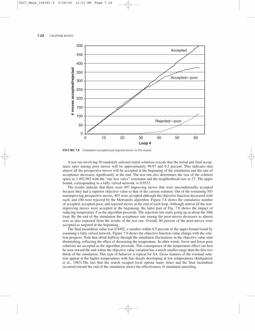
The results indicate that there were 497 improving moves that were unconditionally acceptedbecause they had a superior objective value to that of the current solution. Out of the remaining 503nonimproving prospective moves, 403 were accepted although the objective function decreased witheach, and 100 were rejected by the Metropolis algorithm. Figure 7.8 shows the cumulative numberof accepted, accepted-poor, and rejected moves at the end of each loop. Although almost all the non-improving moves were accepted at the beginning, the latter part of Fig. 7.8 shows the impact ofreducing temperature T as the algorithm proceeds. The rejection rate starts going up at about the 30thloop. By the end of the simulation the acceptance rate among the poor-moves decreases to almostzero as also expected from the results of the test run. Overall, 80 percent of the poor-moves wereaccepted as targeted at the beginning.

The final incumbent value was 0.9492, a number within 0.5 percent of the upper bound found byassuming a fully valved network. Figure 7.9 shows the objective function value change with the solu-tion progress. Note that about halfway through the simulation fluctuations in the objective value startdiminishing, reflecting the effect of decreasing the temperature. In other words, fewer and fewer poorsolutions are accepted as the algorithm proceeds. This consequence of the temperature effect can bestbe seen toward the end where the objective value variation has a much smaller range than the first twothirds of the simulation. This type of behavior is typical for SA. Gross features of the eventual solu-tion appear at the higher temperatures with fine details developing at low temperatures (Kirkpatricket al., 1983).The fact that the search escaped local optima many times and the final incumbentoccurred toward the end of the simulation shows the effectiveness of simulated annealing.

7.24 CHAPTER SEVEN

0

50

100

150

200

250

300

350

400

450

500

# m

ove

s ac

cep

ted

/rej

ecte

d

0 10 20 30 40 50 60

Loop #

Accepted

Accepted—poor

Rejected—poor

FIGURE 7.8 Cumulative accepted and rejected moves in SA search.

Ch07_Mays_144381-9 9/28/04 12:01 AM Page 7.24

Figure 7.10 shows the valve scheme for the final incumbent solution. Note that the “one lessvalve” constraint is preserved throughout the simulation and the optimal solution shown is differentfrom the least-cost solution with respect to only two valve locations. In other words, the optimalsolution is also one of the least-cost solutions as expected.

REFERENCES

AWWA (1986). Introduction to Water Distribution, American Water Works Association, Denver, Colo.

Bhave, P. R. (1991). Analysis of Flow in Water Distribution Networks, Technocomic, Lancaster, Pa.

Bouchart, F. and I. Goulter (1991). “Reliability Improvements in Design of Water Distribution Networks RecognizingValve Location,” Water Resources Research, American Geophysical Union, 27(12):3029–3040.

Bouchart, F. and I. Goulter (2000). “Chapter 18: Reliability Analysis for Design,” in Water Distributions SystemsHandbook, L. W. Mays, ed., McGraw-Hill, New York.

Chin, D. A. (2000). Water Resources Engineering, Prentice-Hall, Upper Saddle River, N.J.

Clark, R. M. (1987). “Applying Water Quality Models, Chapter 20,” in Computer Modeling of Free-Surfaceand Pressurized Flows,” M. H. Chaudhry and L. W. Mays, eds. Kluwer Academic, Dordrecht, Netherlands,pp. 581—612.

OPTIMAL LOCATION OF ISOLATION VALVES 7.25

0.945

0.940

0.935

0.930

0.925

Ob

ject

ive

valu

e

FIGURE 7.9 Accepted solution values for Pmin � 15 psi.

Ch07_Mays_144381-9 9/28/04 12:01 AM Page 7.25

Clark, R. M., J. Q. Adams, and R. M. Miltner (1987). “Cost and Performance Modeling for Regulatory DecisionMaking,” Water, 28(3):26/24/040—27.

Clark, R. M., C. L. Stafford, and J. A. Goodrich (1982). “Water Distribution Systems: A Spatial and CostEvaluation,” Journal of Water Resources Planning and Management, ASCE, 108(8):243–256.

Crow, L. H. (1974). “Reliability Analysis for Complex, Repairable Systems in Reliability and Biometry.” SIAM,F. Proschan and R. J. Serfling, eds. Philadelphia, 379–410.

Cullinane, M. J. (1986). “Hydraulic Reliability of Urban Water Distribution Systems,” Proceedings, Water Forum1986: World Water Issues in Evolution, ASCE, New York, pp. 1264–1271.

Fujiwara, O. and A. U. De Silva (1990). “Algorithm for Reliability-Based Optimal Design of Water Networks.”Journal of Environmental Engineering, 116(3):575–587.

Gleick, P. H. (1993). Water in Crisis, A Guide to the World’s Freshwater Resources, Oxford University Press,New York.

Gleick, P. H. (1998). The World’s Water 1998–1999, The Biennial Report on Freshwater Resources, Island Press,Washington, D.C.

Gupta, R. and P. R. Bhave (1996). “Comparison of Methods for Predicting Deficient Network Performance,”Journal of Water Resources Planning and Management, ASCE, 122(3):214–217.

Gupta, R. and P. R. Bhave (1997). “Closure of ‘Comparison of Methods for Predicting Deficient NetworkPerformance’,” Journal of Water Resources Planning and Management, ASCE, 123(6):370.

Kirkpatrick, S., C. Gelatt, and M. Vecchi (1983). “Optimization by Simulated Annealing,” Science, 220:671–680.

Mays, L. W., ed. (1989). Reliability Analysis of Water Distribution Systems, American Society of Civil Engineers,New York.

Mays, L. W., ed. (2000) Water Distribution Systems Handbook, McGraw-Hill, New York.

Mays, L. W., ed. (2002). Urban Water Supply Handbook, McGraw-Hill, New York.

Mays, L. W., ed. (2004a). Urban Water Supply Management Tools, McGraw-Hill, New York.

Mays, L. W., ed. (2004b). Water Supply Systems Security, McGraw-Hill, New York.

7.26 CHAPTER SEVEN

FIGURE 7.10 Optimal valve layout for example network I from SA.

Ch07_Mays_144381-9 9/28/04 12:01 AM Page 7.26

Ozger, S. (2003). “A Semi-Pressure-Driven Approach to Reliability Assessment of Water Distribution Networks,”Ph.D. dissertation, Department of Civil and Environmental Engineering, Arizona State University, Tempe, Ariz.

Ross, S. M. (1985). Introduction to Probability Models, Academic, New York.

Rossman, L. A. (1994). “EPANET Users Manual,” Drinking Water Research Division, Risk Reduction EngineeringLaboratory, Office of Research and Development, U.S. Environmental Protection Agency, Cincinnati, Ohio.

Rossman, L. A. (2000). “EPANET Users Guide,” Drinking Water Research Division, Risk Reduction EngineeringLaboratory, Office of Research and Development, U.S. Environmental Protection Agency, Cincinnati, Ohio.

Rossman, L. A. (2001). “Thread: Modeling Demands,” MIKE NET Support Forum. http://www.bossintl.com/forums.

Shinstine, D. S., I. Ahmed, and K. Lansey (2002). “Reliability/Availability Analysis of Municipal Water DistributionNetworks: Case Studies,” Journal of Water Resources Planning and Management, ASCE, 128(2):140–151.

Tabesh, M. (1998). “Implications of the Pressure Dependency of Outflows on Data Management, MathematicalModelling and Reliability Assessment of Water Distribution Systems,” PhD thesis, University of Liverpool,Liverpool, England.

Tanyimboh, T. T. and M. Tabesh (1997). “Discussion of ‘Comparison of Methods for Predicting Deficient NetworkPerformance,’” Journal of Water Resources Planning and Management, ASCE, 123(6):369–370.

Tanyimboh, T. T., R. Burd, R. Burrows, and M. Tabesh (1999). “Modelling and Reliability Analysis of WaterDistribution Systems,” Water Science Technology, 39(4):249–255.

Tanyimboh, T. T., M. Tabesh, and R. Burrows (2001). “Appraisal of Source Head Methods For Calculating Reliabilityof Water Distribution Networks,” Journal of Water Resources Planning and Management, ASCE, 127(4):206–213.

Tobias, P. A. and D. C. Trindade (1995). Applied Reliability, 2d ed., Chapman & Hall/CRC, New York.

Walski, T. M. (2000). “Chapter 17: Maintenance and Rehabilitation/Replacement,” Water Distributions SystemsHandbook, L. W. Mays, ed., McGraw-Hill, New York.

Wood, D. J. (1980). “User’s Manual—Computer Analysis of Flow in Pipe Networks Including Extended PeriodSimulation,” Department of Civil Engineering, University of Kentucky, Lexington, Ky.

Ysusi, M. A. (2000). “Chapter 3: System Design: An Overview,” Water Distributions Systems Handbook, L. W.Mays, ed., McGraw-Hill, New York.

OPTIMAL LOCATION OF ISOLATION VALVES 7.27

Ch07_Mays_144381-9 9/28/04 12:01 AM Page 7.27

Ch07_Mays_144381-9 9/28/04 12:01 AM Page 7.28