Chapter 7 Green Logistics - Home | Professor Yossi …...Green Logistics Edgar E. Blanco and Yossi...

147© Yann Bouchery, Charles J. Corbett, Jan C. Fransoo, and Tarkan Tan 2017 Y. Bouchery et al. (eds.), Sustainable Supply Chains, Springer Series in Supply Chain Management 4, DOI 10.1007/978-3-319-29791-0_7

Chapter 7Green Logistics

Edgar E. Blanco and Yossi Sheffi

7.1 Introduction

Logistics encompasses the business processes that plan, control, and implement the flow of goods and related information between points of origin and points of con-sumption to meet customer demand. It does so by managing transportation, ware-housing, and inventory decisions across the company and, whenever possible, across its supply chain.

Traditionally, logistics decisions have been driven by minimizing cost, maximiz-ing profitability, or achieving customer service targets. As companies have added sustainability goals to their business objectives, there has been an increased interest in mitigating the social and environmental impact of their products and operations. This new focus has also impacted the field of logistics: transportation providers are expected to reduce greenhouse gas emissions from their vehicles, warehouse man-agers have focused on waste and energy reduction strategies, and products are rede-signed to increase recyclability and reuse, which require different inventory planning needs.

Green Logistics refers to the systematic measurement, analysis, and, ultimately, mitigation of the environmental impact of logistics activities. This effort to mitigate environmental externalities in logistics activities includes reducing of consumption of nonrenewable energy sources, air emissions (e.g., particulate matter), greenhouse gas emissions, and waste. Some of these efforts may be technological, such as

E.E. Blanco (*) MIT Center for Transportation & Logistics, Cambridge, MA, USA

Walmart Stores, San Bruno, CA, USAe-mail: [email protected]

Y. Sheffi MIT Center for Transportation & Logistics, Cambridge, MA, USAe-mail: [email protected]

148

replacing vehicle fleets from diesel to hybrid or replacing cardboard boxes with returnable totes. Other strategies involve better ways to plan and execute the move-ment of goods, such as increasing the utilization of trucks while maintaining inven-tory levels under control; or using modes of transportation that have lower greenhouse gas emissions. Finally, some green logistics initiatives may be in sup-port of larger business environmental goals, such as increasing reverse logistics activities to recover and reuse more of the products delivered to customers.

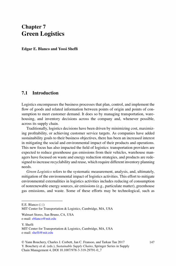
The International Energy Agency (IEA 2009) estimates that transport as a whole accounts for 19 % of global energy use and 23 % of energy-related carbon dioxide (CO2) emission. Under current policies and technology trends, these emissions are expected to grow 50 % by 2030 and between 80 and 130 % by 2050 from 2007 lev-els. Within the transportation sector, freight, especially trucking, is expected to experience the fastest growth. In the USA, medium and heavy-duty freight trucks account for more than 60 % of the freight transportation emissions and are growing faster than any other mode (Greene and Plotkin 2001). Figure 7.1 provides an over-all estimate of CO2 emissions from freight transport and logistics activities. Transport is responsible for about 90 % of these emissions. The main focus of this chapter on green logistics consequently relates to freight transportation.

This chapter is organized as follows. Section 7.2 describes the main environmen-tal impacts of logistic operations, namely greenhouse gases, pollution, noise, vibra-tion, and packaging waste. Details on how these impacts could be estimated and

0

500

1000

1500

2000

2500

3000

Meg

aton

nes

of C

O2e

per

yea

rGHG Emissions by

Logistics and Transport Activity

Road Freight Ocean Freight Air Freight Rail Freight Logistics Buildings

300

Fig. 7.1 GHG emissions of logistics and transport activity (Data source: WEF, 2009)

E.E. Blanco and Y. Sheffi

149

their relative importance is discussed. Section 7.3 focuses on the importance and subtleties of measuring green logistics. Section 7.4 introduces the various green logistics strategies available to mitigate these impacts. These strategies are pre-sented within a framework of decision-making, including a discussion on how to leverage two important modeling approaches to achieve green logistics: network design and vehicle routing. Using real-life success stories, Sect. 7.5 discusses how organizations collaborate to implement green logistics in practice. We conclude with a discussion on other strategies and relevant aspects of a sound green logistics strategy.

7.2 The Environmental Impact of Logistics

As goods flow from origins to destinations through the logistics network, they are moved in conveyances (e.g., planes, trucks, ships, motorcycles) powered by fossil fuels (e.g., diesel, petrol). During the engine combustion process, visible and invis-ible gasses are emitted through exhaust pipes that impact the local, regional, and global atmospheric composition, ranging from local air, water, or soil pollution to global climate change. Energy used during storage and handling of goods also impacts the atmosphere, albeit not always directly, but indirectly through nonrenew-able energy use. The transport conveyances also generate noise and vibration as they navigate roads, highways, and waterways, thereby affecting human and wild-life quality of life. Finally, additional packaging and materials is used to preserve the integrity of products before they reach customers. Inadequate disposal or excess waste of this additional protective packaging is another potential environmental impact of logistics.

In this section we will describe the four main environmental impacts of transpor-tation operations in logistics: Greenhouse gas (GHG) emissions that affect global climate, pollution of air quality and water ways, noise and vibration that affect human health, and packaging waste that increases pressure on landfills.

7.2.1 GHG Emissions

Greenhouse gases trap heat, making the planet warmer. The Intergovernmental Panel on Climate Change (IPCC) identifies transportation activities as producing three direct greenhouse gases: carbon dioxide (CO2), methane (CH4), and nitrous oxide (N2O). The combustion of transport fuels produces relatively little carbon in non-CO2 gases. The impact of each of these greenhouse gases is expressed in terms of carbon dioxide equivalents (CO2e), a process commonly referred to as carbon footprinting. (For more on carbon footprinting, see also Chap. 3 by Boukherroub et al. (2017)).

7 Green Logistics

150

As mentioned earlier, more than 90 % of the GHG emissions in logistics are due to freight transportation. For each mode of transportation in a logistics network (road, railways, water-borne navigation, aviation) the IPCC recommends a fuel- based approach to measuring emissions due to the fairly consistent estimates of the amount of greenhouse gases produced by combustion of each type of fuel. This approach is also known as energy-based calculation, and it is the most reliable for CO2, the primary greenhouse gas from transportation, representing an estimated 97 % of GHG emissions from road (IPCC 2006) and 98 % from marine transporta-tion (IMO 2009).

If total fuel consumption is known, CO2 emissions can be computed as described in Eq. 7.1 by multiplying the total fuel used by the conveyance multiplied by the emissions factor for that fuel.

(7.1)

CH4 and N2O are best estimated using distance traveled plus emissions produced during cold start of the conveyance. It necessitates a more detailed breakdown of the data, requiring distance traveled and emissions factors by fuel type, vehicle type, emission control technology, and operating conditions such as road types. This is shown in Eq. 7.2.

(7.2)

Table 7.1 illustrates the resulting emissions for 1000 gal of fuel, using emission factors from various sources. Note that the resulting calculations are affected by the


151

Table 7.1 GHG emissions calculated for 1000 gal of fuel

Fuel GHGs Source Emissions included Results Units

Diesel CO2 UK Defra Pump-to-wheel 9998 kg CO2

Diesel CO2 US EPA Pump-to-wheel 10,150 kg CO2

Diesel CO2, CH4, N2O GHG Protocol (EPA) Pump-to-wheel 10,159 kg CO2e

Biodiesel CO2 GHG Protocol (EPA) Pump-to-wheel 0 kg CO2

Biodiesel CO2 (biomass) GHG Protocol (EPA) Pump-to-wheel 9460 kg CO2

Diesel CO2, CH4, N2O GREET Well-to-wheel 12,933 kg CO2e

Biodiesel CO2, CH4, N2O GREET Well-to-wheel 2964 kg CO2e

Source: Craig et al. (2013)

type of GHG gas included, as well as the scope of emissions included in the calculation, from the pump-to-wheel or well-to-wheel/life-cycle (see Sect. 7.3.2 for a discussion on emission scopes).

7.2.1.1 Activity-Based Calculations

Equations 7.1 and 7.2 from the IPCC guidelines assume total fuel consumption numbers are readily available or easy to estimate. Although this may be the case at the national or regional level (e.g., total oil imports, total petrol sales) or to convey-ance owners that keep track of fuel purchases, this data is often not accessible to third-party logistics providers, manufacturers or retailers who make logistics deci-sions. Moreover, logistics decisions are not made at the conveyance level (e.g., truck, vessel, locomotive) but rather at the shipment level (e.g., box, carton, pallet) or at another planning metric (e.g., kilogram, cubic feet, or tonne).

Activity-based methods work by estimating the fuel consumed during transpor-tation based on vehicle characteristics, or combining fuel consumption data with activity data to calculate average efficiency numbers. Like fuel-based methods, these methods will be sensitive to the choice of fuel emissions factors.

Distance Based

The simplest approach to estimating emissions from activity data is to use the dis-tance traveled multiplied by the average fuel consumption of the vehicle or convey-ance. Together, these produce an estimate of the fuel consumed, which can then be used to estimate GHG emissions by choosing an appropriate factor, as discussed in the fuel-based methods. A number of different approaches are used in practice to estimate vehicle-distance emissions factors, generally varying in the level of preci-sion they provide.

The GHG Protocol provides default emissions factors per mile for a number of vehicle types, using both US and UK numbers. The emissions factors for US vehi-cles are based on assumed average vehicle efficiency for a variety of vehicle types

7 Green Logistics

152

(Heavy Duty, Light Duty, Passenger Cars, Motorbikes, etc.) to determine fuel consumption, and the standard factors for CO2, CH4, and N2O from the US Environmental Protection Agency (EPA) discussed in the fuel-based section. Numbers in the UK are based on surveys of fuel consumption in vehicle fleets. The fuel consumption data is combined with the UK Department for Environment, Food & Rural Affairs (Defra) standard CO2 factor to produce an emission factor consider-ing only CO2 on a per-kilometer basis.

Other sources have focused more on a single mode type to provide more precise levels of emissions factors. The EPA’s SmartWay program (see Sect. 7.5.4) collects data from a number of different carriers. It employs a fuel-based methodology to calculate emissions from the carriers, and combines this with activity data supplied by the carriers to calculate distance-based emission factors at the individual carrier level. This is then used to create a hierarchy of emissions factors, from which a user can select emission factors for a mode (truck, rail, multi-modal, logistics), a cate-gory within the mode (such as package, truckload/dry van, refrigerated, and others within the truck category), and finally a specific carrier within that category. A single company may have a number of different emissions factors, one for each category of business for which it reported data.

The Network for Transport and Environment (NTM) program does not collect specific data from carriers, but rather uses the ARTEMIS simulation tool to calcu-late fuel consumption for a number of different scenarios (NTM 2010). These sce-narios account for different sizes of vehicles, percent loaded, road type, and driving conditions. By using these scenarios and an associated fuel-based emissions factor, a range of emissions factors can be calculated. In each case, the emissions are cal-culated using a straightforward multiplication of the distance and the vehicle- specific emissions factor.

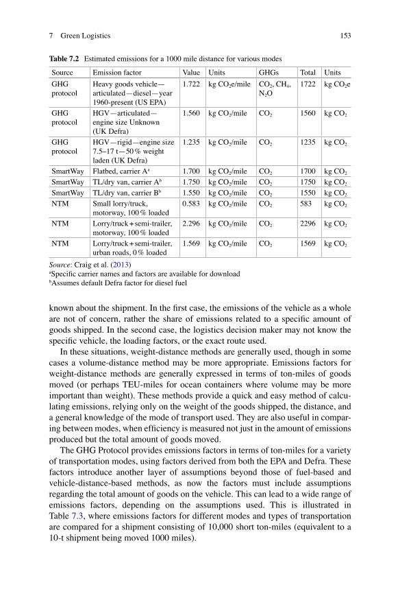
Table 7.2 shows a summary of the results of using a number of different types of factors to calculate the emissions from a 1000-mile trip.

Despite little variation between emissions factors for diesel fuel, the emissions estimated for a specific trip using activity-based distance methods can vary consid-erably. This is true even for vehicles in the same class, as the NTM factors shown for a truck + semi-trailer range from 1.6 to 2.3 depending on the load factor and road type. The EPA SmartWay factors illustrate the correlation of emissions by specific carrier and type of freight.

This demonstrates important points about the precision of the emissions factors used. Estimations of fuel consumed can vary considerably, and therefore even if consistent fuel-based factors are used, the results obtained from activity-based data are sensitive to the assumptions regarding vehicle operating conditions (e.g., terrain, amount of cargo, driver proficiency).

Weight-Distance Based

Despite the ease of using vehicle-distance factors and the availability of a wide range of emissions factors, it is still inadequate for logistics analysis when using shared modes of transportation or when only the bare minimum of information is


153

known about the shipment. In the first case, the emissions of the vehicle as a whole are not of concern, rather the share of emissions related to a specific amount of goods shipped. In the second case, the logistics decision maker may not know the specific vehicle, the loading factors, or the exact route used.

In these situations, weight-distance methods are generally used, though in some cases a volume-distance method may be more appropriate. Emissions factors for weight-distance methods are generally expressed in terms of ton-miles of goods moved (or perhaps TEU-miles for ocean containers where volume may be more important than weight). These methods provide a quick and easy method of calcu-lating emissions, relying only on the weight of the goods shipped, the distance, and a general knowledge of the mode of transport used. They are also useful in compar-ing between modes, when efficiency is measured not just in the amount of emissions produced but the total amount of goods moved.

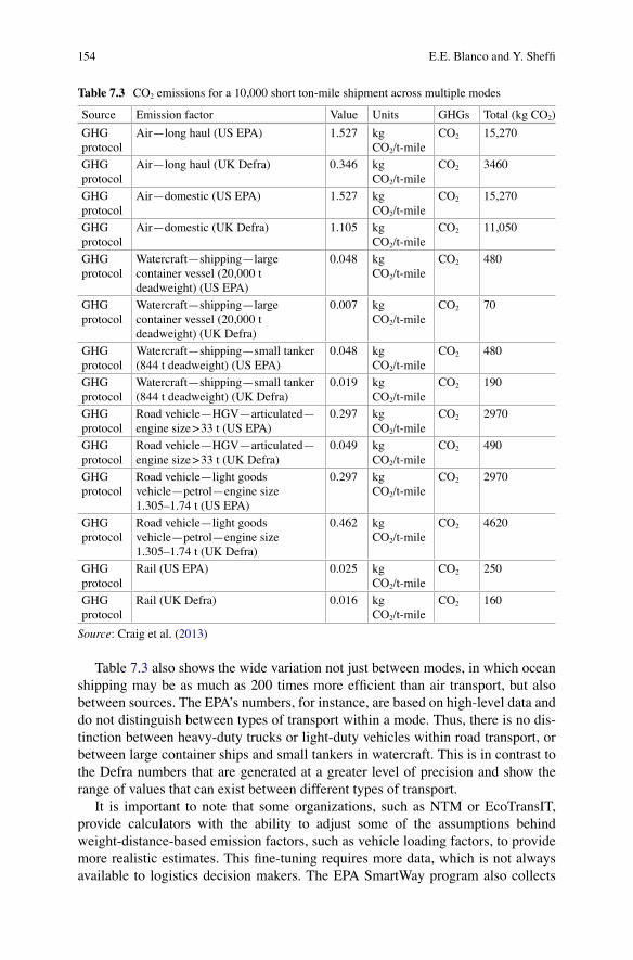
The GHG Protocol provides emissions factors in terms of ton-miles for a variety of transportation modes, using factors derived from both the EPA and Defra. These factors introduce another layer of assumptions beyond those of fuel-based and vehicle- distance-based methods, as now the factors must include assumptions regarding the total amount of goods on the vehicle. This can lead to a wide range of emissions factors, depending on the assumptions used. This is illustrated in Table 7.3, where emissions factors for different modes and types of transportation are compared for a shipment consisting of 10,000 short ton-miles (equivalent to a 10-t shipment being moved 1000 miles).

Table 7.2 Estimated emissions for a 1000 mile distance for various modes

Source Emission factor Value Units GHGs Total Units

GHG protocol

Heavy goods vehicle—articulated—diesel—year 1960-present (US EPA)

1.722 kg CO2e/mile CO2, CH4, N2O

1722 kg CO2e

GHG protocol

HGV—articulated—engine size Unknown (UK Defra)

1.560 kg CO2/mile CO2 1560 kg CO2

GHG protocol

HGV—rigid—engine size 7.5–17 t—50 % weight laden (UK Defra)


SmartWay Flatbed, carrier Aa 1.700 kg CO2/mile CO2 1700 kg CO2

SmartWay TL/dry van, carrier Ab 1.750 kg CO2/mile CO2 1750 kg CO2

SmartWay TL/dry van, carrier Bb 1.550 kg CO2/mile CO2 1550 kg CO2

NTM Small lorry/truck, motorway, 100 % loaded


NTM Lorry/truck + semi-trailer, motorway, 100 % loaded


NTM Lorry/truck + semi-trailer, urban roads, 0 % loaded


Source: Craig et al. (2013)aSpecific carrier names and factors are available for downloadbAssumes default Defra factor for diesel fuel

7 Green Logistics

154

Table 7.3 also shows the wide variation not just between modes, in which ocean shipping may be as much as 200 times more efficient than air transport, but also between sources. The EPA’s numbers, for instance, are based on high-level data and do not distinguish between types of transport within a mode. Thus, there is no dis-tinction between heavy-duty trucks or light-duty vehicles within road transport, or between large container ships and small tankers in watercraft. This is in contrast to the Defra numbers that are generated at a greater level of precision and show the range of values that can exist between different types of transport.

It is important to note that some organizations, such as NTM or EcoTransIT, provide calculators with the ability to adjust some of the assumptions behind weight-distance-based emission factors, such as vehicle loading factors, to provide more realistic estimates. This fine-tuning requires more data, which is not always available to logistics decision makers. The EPA SmartWay program also collects

Table 7.3 CO2 emissions for a 10,000 short ton-mile shipment across multiple modes

Source Emission factor Value Units GHGs Total (kg CO2)

GHG protocol

Air—long haul (US EPA) 1.527 kg CO2/t- mile

CO2 15,270

GHG protocol

Air—long haul (UK Defra) 0.346 kg CO2/t- mile

CO2 3460

GHG protocol

Air—domestic (US EPA) 1.527 kg CO2/t- mile

CO2 15,270

GHG protocol

Air—domestic (UK Defra) 1.105 kg CO2/t- mile

CO2 11,050

GHG protocol

Watercraft—shipping—large container vessel (20,000 t deadweight) (US EPA)

0.048 kg CO2/t- mile

CO2 480

GHG protocol

Watercraft—shipping—large container vessel (20,000 t deadweight) (UK Defra)


CO2 70

GHG protocol

Watercraft—shipping—small tanker (844 t deadweight) (US EPA)


CO2 480

GHG protocol

Watercraft—shipping—small tanker (844 t deadweight) (UK Defra)


CO2 190

GHG protocol

Road vehicle—HGV—articulated—engine size > 33 t (US EPA)


CO2 2970

GHG protocol

Road vehicle—HGV—articulated—engine size > 33 t (UK Defra)


CO2 490

GHG protocol

Road vehicle—light goods vehicle—petrol—engine size 1.305–1.74 t (US EPA)


CO2 2970

GHG protocol

Road vehicle—light goods vehicle—petrol—engine size 1.305–1.74 t (UK Defra)


CO2 4620

GHG protocol

Rail (US EPA) 0.025 kg CO2/t- mile

CO2 250

GHG protocol

Rail (UK Defra) 0.016 kg CO2/t- mile

CO2 160

Source: Craig et al. (2013)


155

similar data by carrier, providing another layer of detail to emission factors. Finally, some logistics operators and transportation companies, such as DHL, FedEx, or Maersk, use their internal proprietary systems and their transportation network information (e.g., total weight or cube moved on a particular transportation lane during a year) and combine it with fuel consumption records of the vehicles or ves-sels, to provide lane-specific distance-weight emission factors, and in some cases, shipper-specific factors for dedicated customers. These factors are often updated annually, although there is a trend toward more frequent reporting. Even these orga-nizations rely on emission factors like the ones listed in Table 7.3, because their shipments may move between trucks, ships, or airplanes for which fuel records are not available or that belong to third parties with less detailed information.

7.2.1.2 Mode-Specific Adjustments

All of the GHG calculation approaches and methods discussed above are applicable to all modes of transportation (road, rail, water-borne, and air). Most salient differ-ences, besides variations in engine technology and type of fuels, are related to the GHG gases included, the quality of data, the allocation of emissions to freight due to capacity sharing (e.g., same vehicle moving people and boxes), and strategies to overcome data limitations.

Rail

The most important variation in rail has to do with the variability of the number of railcars (empty and full) being pulled by a single locomotive. In theory the amount of fuel consumed during any journey or leg can be tracked and allocated to the cargo being hauled on that specific leg, thereby creating movement-specific factors. In practice, however, rail operators plan their movements and balance on a network perspective. Thus, it only makes sense to look at emissions from a series of inter-connected networks or services and to measure the total amount of fuel and cargo moved through that rail network, as opposed to individual legs. These calculations are often done annually but could also be done on a monthly or quarterly basis, aligned with rail operator planning cycles.

Water-Borne Navigation

Some water-borne navigation providers, such as barges, operate in a similar fashion as long-haul vehicles, albeit through a smaller transportation network: rivers and canals. For these providers, trip-based estimations are sensible: measuring the total fuel consumed between origin and destination and allocating the emissions to the amount of cargo loaded. Because adjustments for empty journeys need to be added and assigned to various trips, emission factors that span more than one journey over a time horizon are often needed.

7 Green Logistics

156

For large ocean-going cargo ships, the situation is very different. Unlike river waterways, ocean shipping companies plan their transportation networks by trade lanes between continents and sub-continents, stringing together multiple trade lanes to provide regular service to various ports. Thus, similar to rail transportation, even though is mathematically possible, it doesn’t make sense to compute GHG emis-sions by looking at port-to-port distances without full understanding of the overall trade-lane dynamics. In addition, given the size of the vessels and the relatively few number of carriers (compared to road transport) the industry has been developing joint efforts to calculate emission factors by trade-lane in a homogeneous way. The Clean Cargo Working Group has been collecting data in collaboration with major shipping companies to provide a homogeneous calculation approach of emissions by trade-lane and ship assignment, if possible.

An additional feature of some water-borne navigation has to do with the relevant unit of measures used by shipping companies to determine the amount of freight being transported: the container. After the invention and wide adoption of the con-tainer, water-borne navigation was transformed to leverage the economic and effi-ciency advantages of the container. As a consequence, all planning and pricing decisions are made in TEU or Twenty-Foot-Equivalent-Units, a volumetric unit of measure equivalent to the total cube of a standard twenty feet container. Although cargo owners may know the total weight inside a particular container, shipping companies often only know (and care) about the TEU. Thus, emission factors com-puted by water-borne transportation are often originally computed in kilograms of CO2-e per TEU-kilometer and then converted into ton-kilometers by using a pre- agreed conversion factor.

Aviation

Sources of emissions for aviation are all civil commercial airplanes, including gen-eral aviation such as agricultural aircraft, private jets, and helicopters. The fuel- based methodology again uses only fuel consumption data and average emission factors to estimate emissions, and is suitable for aircraft using aviation gasoline or when operational data for jet-fueled vehicles are not available. A fuel-based approach can also be estimated by calculating emissions separately for the cruise phase of a flight and the landing/take-off (LTO) phase. This requires knowing the number of LTOs and separating the fuel consumed during this phase from the cruise phase, but it allows for using emissions factors that capture differences in emissions, specially CH4 and N2O, during these phases.

Distance-based methods can be based on origin-destination (OD) data or full flight trajectory information. The OD approach accounts for different flight dis-tances, which changes the relative impact of the LTO phase compared to the cruise phase. The full flight trajectory model uses aircraft—and engine-specific perfor-mance information over the entire flight, requiring engine performance modeling.

An additional complexity in aviation has to do with the allocation of emissions between people and freight, because they share the same airplane when cargo is loaded onto commercial flights. The most accurate way to allocate emissions is to


157

use the ratio of weight used by passengers (and their bags) vs. the weight of freight, because weight is what determines the amount of fuel consumed during the flight. However, airlines do not plan routes using this criteria; instead, they evaluate the economics of each flight and the revenue from the various services they offer. Thus, emissions could be allocated based on the revenue of passenger vs. freight as a proxy to the planning approach. Even this approach has further complications because first class, business, and economy fares are sold at different rates on every flight as part of yield management strategy, varying the revenue profile of each flight and “underutilizing” the maximum weight potential of a flight. A third approach would be to allocate a fixed share of emissions to freight on a flight, recognizing that airlines often plan and balance their network using revenue targets. The EN 16258 (see Sect. 7.3.3) has favored this latter approach, recommending a factor between 70 and 80 % of emissions to be allocated to freight on commercial flight, regardless of actual load capacity or revenue. This number, although arbitrary, is a result of a consultation process with experts from academia and industry trying to balance accuracy of emissions with practical business matters of data collection and consis-tency in reporting.

7.2.1.3 Carbon Footprint Calculations in Transportation: A Primer

As mentioned at the beginning of this section, the most accurate method for calcula-tion carbon footprints of transportation emissions is to use fuel records of the con-veyance (see Eq. 7.1).

However, since most transportation activities often involve multiple organiza-tions (e.g., shipper and carrier) and may further involve other intermediaries such as freight forwarders or 3PLs, weight-distance activity-based calculations are more commonly used in practice (see Sect. 7.2.1.1). The carbon footprint calculation using this approach is often estimated as a function of the shipment weight (w) or volume (v), the distance (d), and a mode-specific emission factor (EF). The most basic relationship is multiplicative as follows:

e d w d w e d v d v( , ) ( , )= × × = × ×EFor EF

The shipment weight is the gross weight of the product being transported (including all primary and secondary packaging). This information is often well known by the shipper. The distance is the total over-the-road, over-the-air, over-the-track, or over- the- waterway distance traveled by the shipment. This number may not always be accurate or easily available for the shipper, but it is often known by the carrier or asset owner, or can be approximated by using over-the-air distances multiplied by an adjustment factor. Such approximations should be avoided (if possible) since they add another level of uncertainty to the calculation.

The final component, the emission factor EF, is the most critical element of this computation. As discussed earlier in this section, there are multiple sources that publish values that are commonly used by practitioners (see Table 7.3). Ideally, these emissions factors should be gathered directly from fuel consumption records

7 Green Logistics

158

from the carrier or vessel operator (see Sect. 7.5.4), but are most commonly a result of carrier surveys, econometric models or engine fuel consumption modeling. Fuel consumption models allow for more accurate functional forms of e(d, w).

The modeling and data collection undertaken by NTM is one of the most com-prehensive and detailed methodologies available to estimate emission factors of transportation. Based on the excellent summary by Hoen et al. (2014a) of NTM recommended calculations, the following sections summarize functional forms of carbon footprint calculations for different modes of transportation. For all calcula-tions, the resulting calculation emissions are expressed in kilograms of CO2. Distance d is expressed in kilometers, weight w in kilograms, and volume v in m3.

Air Transport

Emissions of air transportation can be estimated as follows:

e d w E dw

Wair ( , ) ( )*( )

= + ××1 1

1 1

l

whereW1 is the aircraft maximum payload in kgλ1 is the aircraft payload utilization % for the specific tripE1 are the emissions (kg of CO2) corresponding to take-off and landing. These emis-sions are a function of the actual aircraft payload W1 1×lϵ1 kilograms of CO2 per kilometer (kg of CO2/km)

For a Boeing 757-200SF, the maximum payload is W1 is 29,029 kg. When fully loaded (e.g., l1 100= % ), E1 4531 182= . and 1 15 363= . . For a payload of l1 75= % of maximum capacity, E1 4041 709= . and 1 15 351= . . Thus, the share of emissions associated to moving a 500 kg shipment for 1000 km will be 342.66 kg CO2 in a fully loaded Boeing 757-200SF and 445.36 kg CO2 if the aircraft will be loaded at 75 % payload capacity.

As mentioned earlier, aircraft payload capacity between passenger and cargo needs to be adequately accounted for. Also, air shipments are often priced volu-metrically. In that case w v= × r , where ρ is the shipment density. This density will vary by product and may also be adjusted for pricing purposes.

Road Transport

Emissions of road transportation can be estimated as follows:

e d w dw

Wroad ( , )( )

= × ××

22 2l


159

whereW2 is the vehicle maximum payload in kgλ2 is the vehicle payload utilization % for the specific tripϵ2 kilograms of CO2 per kilometer (kg of CO2/km).

Commonly used transport vehicles (tractor+trailer) have a maximum payload W2 of 26,000 kg. To estimate ϵ2, NTM recommends taking into account fuel effi-ciency, type of road, load factor, and terrain slope. NTM estimates that diesel con-sumption for an unloaded freight vehicle with a payload capacity of 26,000 kg is 0.226, 0.230, and 0.288 L per km for highway, rural, and city environments, respec-tively. At the other extreme, a fully loaded vehicle consumes 0.360, 0.396, and 0.504 L per km in highway, rural, and city roads. Other load factors may be linearly interpolated between these numbers. Thus, for a load factor of 70 %, fuel consump-tion will be 0.3198, 0.3462, and 0.4392 L per km for highway, rural, and city roads, respectively. Assuming diesel emissions are 2.621 kg CO2 per L, ϵ2 for a l2 70= % loaded vehicle will be given by 2 621 0 3198 0 8382. . .⋅ = kg CO2 per km. An addi-tional adjustment to fuel consumption may be applied to take into account the steep-ness of the terrain. For instance, Hoen et al. (2014a) estimate a European wide adjustment of an additional 5 % to account to terrain. Thus 2 0 8382 1 05 0 8801= ⋅ =. . . .

Therefore, the share of emissions associated to moving a 500 kg shipment for 1000 km will be 11.85 kg CO2 in a 70 % utilized 26,000 kg diesel powered vehicle. Note that for road transport, the allocation of empty miles have a noticeable impact on final shipment emission calculations.

Rail Transport

Since only a handful of national rail operators provide rail transport service by country, it is often most reliable to obtain the emission factor directly from rail transport companies. These factors take into account overall locomotive efficiency, including electric and diesel powered technology, as well as required boxcar repo-sitioning throughout the network. Thus, emissions can be simply calculated as follows:

e d w d wrail ( , ) = ⋅ ⋅3

whereϵ3 kilograms of CO2 per kilometer (kg of CO2/kg-km)

The EPA estimates this number to be 1.713 10−5 kg of CO2 per kg-km for the US rail network. Hoen et al. (2014a) present a detailed derivation of rail emission factor for Europe, that takes into account a combination of electric and diesel power dis-tance and hilly terrain. The resulting value was 2 223 10 5. ⋅ − kg of CO2 per kg-km.

7 Green Logistics

160

Water Transport

Emissions of inland water transportation can be estimated as follows:

e d w dw

Wwater FC FE( , )( )

= × × ××4 4

4 4l

whereW4 is the total vessel capacity in kg, TEU, or meters (for RORO vessels)λ4 is the vessel payload utilization % for the specific tripFC4 is the vehicle fuel consumption in L per kmFE4 are the fuel emissions in kg of CO2 per L

The cargo capacity of an inland cargo vessel is 3,840,000 kg. Inland cargo ves-sels often have low utilization levels, close to 50 %. Vessel fuel consumption is in the order of 0.007 t of diesel per km and diesel emissions of approximately 3178 kg of CO2 per t of diesel. Using these parameters, the share of emissions associated to moving a 500 kg shipment for 1000 km via inland waterways will be 5.79 kg CO2.

In the case of ocean shipping, it is often advised to use carrier-specific emission factors, such as the ones published by the Clean Cargo Working Group (CCWG), although similar calculations as the ones used above can be estimated by adjusting the fuel type used (often bunker fuel oil).

7.2.2 Pollution

Pollution is the introduction of a substance—solid, liquid, or gas—into a system that can have adverse consequences on humans or the natural ecosystem. In the case of logistics and transportation, the most important environmental impacts are due to air and water pollution generated during the operation of trucks, airplanes, locomo-tives, and vessels. Unlike GHG emissions that have global effects, pollution impacts tend to be local to cities, ports, trade lanes, or freight corridors, although pollutants can also travel long distances and have global effects.

7.2.2.1 Air Pollution

The use of internal combustion engines in trucks, airplanes, ships, and locomotive engines that move freight is the major source of air pollution. There are six common air pollutants, also known as “criteria pollutants” in combustion: particle pollution (often referred to as particulate matter), ground-level ozone, carbon monoxide, sul-fur oxides, nitrogen oxides, and lead (EPA 2015a):

• Ground-level ozone is not emitted directly into the air, but it is created by chemi-cal reactions between oxides of nitrogen (NOx) and volatile organic compounds (VOC) in the presence of sunlight.


161

• Particulate matter (PM) is a mixture of extremely small particles and liquid droplets. PM is made up of a number of components, including acids (such as nitrates and sulfates), organic chemicals, metals, and soil or dust particles. The size of particles is directly linked to their potential for causing health problems. The EPA regulations focuses on particles that are 10 μm (PM10) in diameter or smaller because those generally pass through the throat and nose and enter the lungs.

• Carbon monoxide (CO) is a colorless, odorless gas emitted from combustion processes. Nationally, and particularly in urban areas, the majority of CO emis-sions to ambient air come from transportation activities (both passenger and freight). CO can cause harmful health effects by reducing oxygen delivery to the body’s organs (like the heart and brain) and tissues. At extremely high levels, CO can cause death.

• Nitrogen Oxides—or NOx—are a family of seven compounds, of which NO2 is the most prevalent form. About 50 % of all NOx come from mobile sources including automobiles, trucks, and vessels (EPA 2014). They are generated dur-ing the combustion process of engines as a function of the ratio of fuel and oxy-gen. In addition to contributing to the formation of ground-level ozone, and fine-particle pollution, NOx are linked with a number of adverse effects on the respiratory system. The amount of NOx can be controlled through several means: engine design, regulating the oxygen and fuel mix, maintaining optimal tempera-ture levels within the engine, changing fuel types, or adding a catalytic converter. All of these actions have an impact on fuel economy, sometimes positive or nega-tive, and they are very dependent on individual engine configurations (EPA 2014).

• Sulfur oxides—or SOx—are highly reactive gases of which sulfur dioxide (SO2) is the most prevalent form in transportation. SOx is linked with a number of adverse effects on the respiratory system. The largest sources of SOx emissions come from fossil fuel combustion at power plants (73 %) and other industrial facilities (20 %). Smaller sources of SOx emissions include industrial processes such as extracting metal from ore, and the burning of high sulfur containing fuels by locomotives, large ships, and non-road equipment. Although maritime trans-portation represents a small share of global SOx emissions, the emissions tend to accumulate in higher concentrations near ports and then travel to neighboring population centers. SOx emissions are increasingly being regulated across Europe and are part of the focus areas of the maritime industry as whole (IMO 2015).

• Lead is a naturally occurring element that can be harmful to humans when ingested or inhaled. Lead poisoning is particularly detrimental to the neurologi-cal development of children. The major sources of lead emissions have histori-cally been from fuels in on-road motor vehicles (such as cars and trucks) and industrial sources. As a result of US and EU regulatory efforts to remove lead from on-road motor vehicle gasoline, emissions of lead from the transportation sector dramatically declined by 95 % between 1980 and 1999, and levels of lead in the air decreased by 94 % between 1980 and 1999. The major sources of lead emissions to the air today are ore and metals processing and piston-engine air-craft operating on leaded aviation gasoline.

7 Green Logistics

162

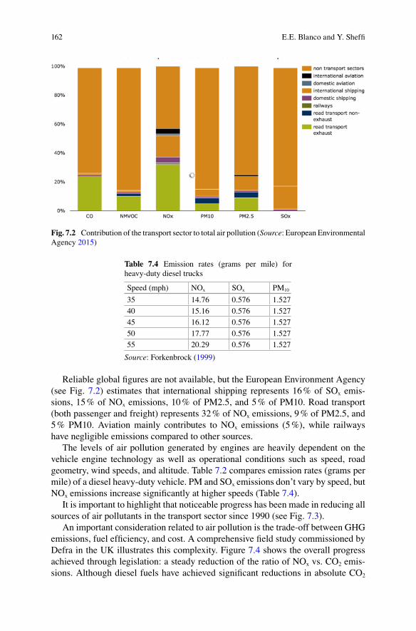
Reliable global figures are not available, but the European Environment Agency (see Fig. 7.2) estimates that international shipping represents 16 % of SOx emis-sions, 15 % of NOx emissions, 10 % of PM2.5, and 5 % of PM10. Road transport (both passenger and freight) represents 32 % of NOx emissions, 9 % of PM2.5, and 5 % PM10. Aviation mainly contributes to NOx emissions (5 %), while railways have negligible emissions compared to other sources.

The levels of air pollution generated by engines are heavily dependent on the vehicle engine technology as well as operational conditions such as speed, road geometry, wind speeds, and altitude. Table 7.2 compares emission rates (grams per mile) of a diesel heavy-duty vehicle. PM and SOx emissions don’t vary by speed, but NOx emissions increase significantly at higher speeds (Table 7.4).

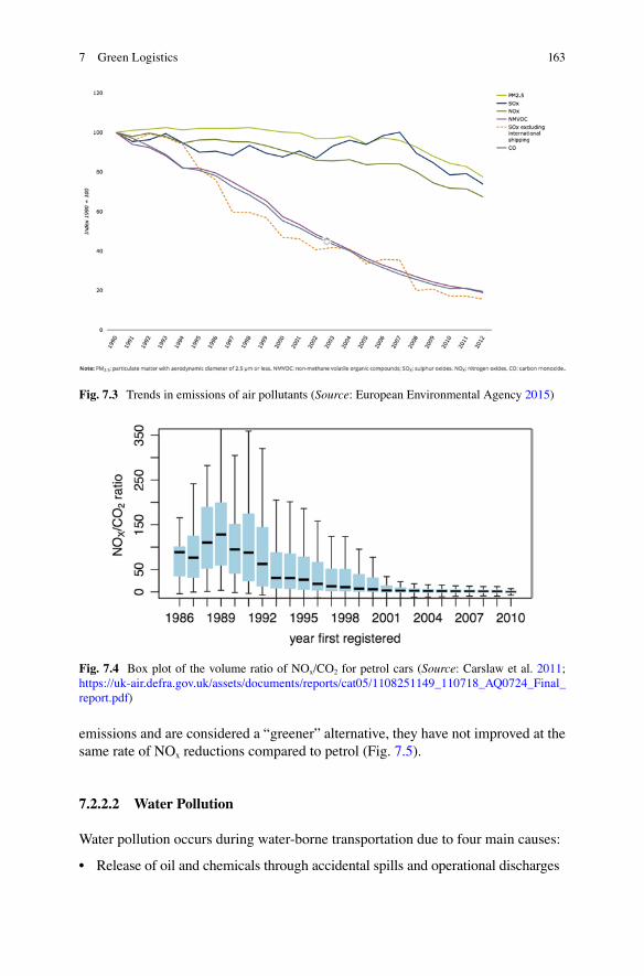
It is important to highlight that noticeable progress has been made in reducing all sources of air pollutants in the transport sector since 1990 (see Fig. 7.3).

An important consideration related to air pollution is the trade-off between GHG emissions, fuel efficiency, and cost. A comprehensive field study commissioned by Defra in the UK illustrates this complexity. Figure 7.4 shows the overall progress achieved through legislation: a steady reduction of the ratio of NOx vs. CO2 emis-sions. Although diesel fuels have achieved significant reductions in absolute CO2

Fig. 7.2 Contribution of the transport sector to total air pollution (Source: European Environmental Agency 2015)

Table 7.4 Emission rates (grams per mile) for heavy-duty diesel trucks

Speed (mph) NOx SOx PM10

35 14.76 0.576 1.527

40 15.16 0.576 1.527

45 16.12 0.576 1.527

50 17.77 0.576 1.527

55 20.29 0.576 1.527

Source: Forkenbrock (1999)


163

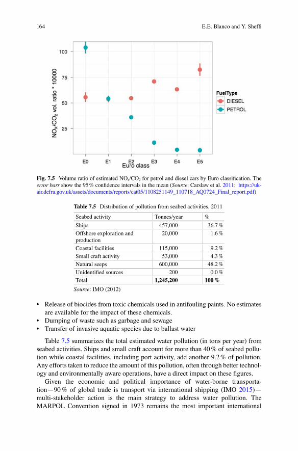
emissions and are considered a “greener” alternative, they have not improved at the same rate of NOx reductions compared to petrol (Fig. 7.5).

7.2.2.2 Water Pollution

Water pollution occurs during water-borne transportation due to four main causes:

• Release of oil and chemicals through accidental spills and operational discharges

Fig. 7.3 Trends in emissions of air pollutants (Source: European Environmental Agency 2015)

Fig. 7.4 Box plot of the volume ratio of NOx/CO2 for petrol cars (Source: Carslaw et al. 2011; https://uk-air.defra.gov.uk/assets/documents/reports/cat05/1108251149_110718_AQ0724_Final_report.pdf)

7 Green Logistics

164

• Release of biocides from toxic chemicals used in antifouling paints. No estimates are available for the impact of these chemicals.

• Dumping of waste such as garbage and sewage• Transfer of invasive aquatic species due to ballast water

Table 7.5 summarizes the total estimated water pollution (in tons per year) from seabed activities. Ships and small craft account for more than 40 % of seabed pollu-tion while coastal facilities, including port activity, add another 9.2 % of pollution. Any efforts taken to reduce the amount of this pollution, often through better technol-ogy and environmentally aware operations, have a direct impact on these figures.

Given the economic and political importance of water-borne transporta-tion—90 % of global trade is transport via international shipping (IMO 2015)—multi-stakeholder action is the main strategy to address water pollution. The MARPOL Convention signed in 1973 remains the most important international

Fig. 7.5 Volume ratio of estimated NOx/CO2 for petrol and diesel cars by Euro classification. The error bars show the 95 % confidence intervals in the mean (Source: Carslaw et al. 2011; https://uk-air.defra.gov.uk/assets/documents/reports/cat05/1108251149_110718_AQ0724_Final_report.pdf)

Table 7.5 Distribution of pollution from seabed activities, 2011

Seabed activity Tonnes/year %

Ships 457,000 36.7 %

Offshore exploration and production

20,000 1.6 %

Coastal facilities 115,000 9.2 %

Small craft activity 53,000 4.3 %

Natural seeps 600,000 48.2 %

Unidentified sources 200 0.0 %

Total 1,245,200 100 %

Source: IMO (2012)


165

treaty instrument covering the prevention of pollution by ships. It sets out regulations dealing with pollution from ships by oil; by noxious liquid substances carried in bulk; by harmful substances carried by sea in packaged form; by sewage; by gar-bage; and with the prevention of air pollution from ships.

7.2.3 Noise and Vibration

The goal of establishing acceptable noise levels is to avoid hearing loss in people over their lifespan, as well as to allow for a comfortable environment to work and rest. In 1974, the EPA determined that a 24-h exposure level of 70 decibels (dB) to be the threshold that will prevent any measurable hearing loss over a lifetime. Levels of 55 dB outdoors and 45 dB indoors were considered as acceptable levels for nor-mal activity. These levels are not peak levels, but 8–24-h averages.

Table 7.6 presents some reference activities and their noise levels.Noise levels related to freight transportation activities (traffic 70 dB, trains 100

dB, and airplanes 130 dB) are above the recommended 70 dB threshold level. This limits the amount of time that freight activities should be allowed near heavily pop-ulation centers. Localities often require stricter noise levels after 6 pm and before 6 am in residential areas, to further mitigate disruption to audible quality of life.

7.2.4 Packaging Waste

Packaging is used to sell, inform, contain, protect, preserve, and transport products (Soroka 1999). After product use, all packaging joins the waste stream.

There are three main types of packaging (Saphire 1994):

• Manufacturer-provided packaging. This is the primary packaging that protects and preserves the product. In some cases, this packaging also informs and helps

Table 7.6 Noise levels of common activities

Activity Noise level

Whisper 30 dB

Normal conversation/laughter 50–65 dB

Vacuum cleaner at 10 ft 70 dB

Washing machine/dishwasher 78 dB

Midtown Manhattan traffic noise 70–85 dB

Motorcycle 88 dB

Train 100 dB

Jackhammer/PowerSaw 85–90 dB

Thunderclap 110 dB

Stereo/boombox 110–120 dB

Nearby jet takeoff 130 dB

Source: NYCDEP (2008)

7 Green Logistics

166

to sell the product contained within. As a customer decides which product to purchase, the packaging has the ability to draw the customer in with its design, image, and attractiveness, regardless of the quality and necessity of a product (Paine 2002).

• Transport packaging or secondary packaging. This type of packaging is used for the sole purpose of moving product around. Most commonly, it is used for bulk handling of product, usually in pallet sizes to facilitate the easy transfer from warehouse to truck or container for shipment across land, air, or sea. Its main function is to protect the contents within from damage from the elements or rough handling.

• Parcel packaging or tertiary packaging. This is used mainly to group primary packages together. It is most frequently used in the retail delivery industry to aggregate customer orders into one box, to facilitate easy delivery through the fulfillment system.

Logistics and transportation activities have direct influence on the design, use, and disposal of secondary and tertiary packaging. Any unnecessary levels or inad-equately disposed packaging is an additional source of waste.

Although detailed statistics are not available, product containers and packaging represent 29 % of the 250 million tons of waste generated in 2010 (EPA 2015a). Approximately 49 % of this waste is recovered (see Table 7.7), which leaves a 51 % opportunity to either reduce packaging use or make sure that it reaches the right recycling facilities.

7.3 Measuring Green Logistics Impacts

Logistics decisions are metrics driven, which means that green logistics models and initiatives require having the right measurements of the various environmental impacts.

Table 7.7 Generation and recovery of containers and packaging

Container and packaging material

Weight generated (tons)

Weight recovered (tons)

Recovery as % of generation

Steel 2.74 1.89 69.0 %

Aluminum 1.90 0.68 35.8 %

Glass 9.36 3.13 33.4 %

Paper and cardboard 37.68 26.85 71.3 %

Plastics 13.68 1.85 13.5 %

Wood 9.94 2.30 23.1 %

Other materials 0.34 Negligible Negligible

Total 75.64 36.70 48.5 %

Source: US EPA (2015b)


167

Pollution, noise, vibration, and waste measurements are technical in nature and can be estimated through specialized equipment. For example, the EPA or the European Union standards (see Table 7.1) are enforced by subjecting technologies to lab and road tests under standard conditions. Driving, weather, terrain, conges-tion, and operational conditions can dramatically change the actual environmental impact of freight operations. In a detailed study of drayage trucks in the port of Genoa, Zamboni et al. (2015) were able to observe differences of more than 50 % in total fuel consumption, NOx and SOx emissions under a variety of speeds and stop patterns. Environmental analysis of logistics operations needs to be very aware of the various assumptions underlying commonly used emission factors. This is par-ticularly important when estimating GHG emissions.

7.3.1 GHG Emission Measurement in Logistics

As discussed in Sect. 7.2.1, there are important variations in emission factors across sources (see Table 7.3). For instance, depending on the assumed (or observed) utili-zation factor of the conveyance and the granularity of data available (e.g., surveys or fuel records), the average fuel consumption per ton of cargo transported will vary significantly. Table 7.8 includes some of the emission factors included in the GHG Protocol. Note that the EPA reference numbers are the same for trucks of various engine sizes, while the Defra numbers vary dramatically between large (over 33 t) and smaller trucks (1.3–1.7 t). This difference is due to the level of detail of data collected by these two agencies at the moment of publication of the GHG Protocol: the EPA was using sector-level aggregated data while Defra had access to vehicle- level surveys. Moreover, these numbers are regularly challenged and updated as more and better data becomes available across the logistics sector (Table 7.8).

Another complexity, especially relevant to GHGs measurements, is what is and what is not included in the emission factors and calculations.

7.3.2 GHG Standards and Scopes1

There are three types of standards that cover GHG impact estimations. If the intent of the measurement is an absolute quantity for a whole company, this is known as Corporate Carbon Footprinting. The most widely known and adopted standard is the GHG Protocol followed by the ISO 14064. If the intent is to measure the GHG impact of an individual product, often from cradle to grave, it is known as Product

1 The GHG Protocol Corporate Standard also includes a scope definition. Although conceptually related, it does not correspond to the scope definition when applied to logistics activities. See Chap. 3 by Boukherroub et al. (2017) for an in-depth discussion of carbon footprinting, including more on the GHG Protocol Scope definitions.

7 Green Logistics

168

Carbon Footprinting. The PAS-2050, ISO 14040, and the GHG Protocol Life Cycle Accounting and Reporting Standards are well-known references. Finally, and most recently, the EN 16258 (VTT 2012) standard for quantifying greenhouse gas emis-sions from freight focus specifically on carbon footprinting in the transportation sector.

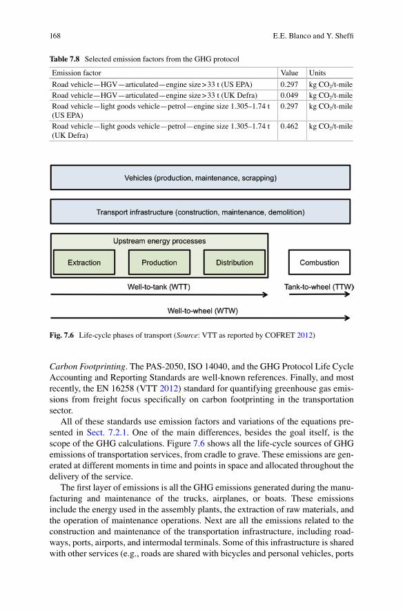
All of these standards use emission factors and variations of the equations pre-sented in Sect. 7.2.1. One of the main differences, besides the goal itself, is the scope of the GHG calculations. Figure 7.6 shows all the life-cycle sources of GHG emissions of transportation services, from cradle to grave. These emissions are gen-erated at different moments in time and points in space and allocated throughout the delivery of the service.

The first layer of emissions is all the GHG emissions generated during the manu-facturing and maintenance of the trucks, airplanes, or boats. These emissions include the energy used in the assembly plants, the extraction of raw materials, and the operation of maintenance operations. Next are all the emissions related to the construction and maintenance of the transportation infrastructure, including road-ways, ports, airports, and intermodal terminals. Some of this infrastructure is shared with other services (e.g., roads are shared with bicycles and personal vehicles, ports

Fig. 7.6 Life-cycle phases of transport (Source: VTT as reported by COFRET 2012)

Table 7.8 Selected emission factors from the GHG protocol

Emission factor Value Units

Road vehicle—HGV—articulated—engine size > 33 t (US EPA) 0.297 kg CO2/t-mile

Road vehicle—HGV—articulated—engine size > 33 t (UK Defra) 0.049 kg CO2/t-mile

Road vehicle—light goods vehicle—petrol—engine size 1.305–1.74 t (US EPA)

0.297 kg CO2/t-mile

Road vehicle—light goods vehicle—petrol—engine size 1.305–1.74 t (UK Defra)

0.462 kg CO2/t-mile


169

are shared with government and military operations) and needs to be properly allocated.

In order to be able to do a complete calculation of the impact of freight transpor-tation, some share of the vehicle and infrastructure emissions should be added to each logistic operation. This is a fairly complex and uncertain calculation that requires very large amounts of data and assumptions. With the exception of life- cycle analysis or product carbon footprint calculations, most of these emissions are not included in GHG calculations in the logistics sector.

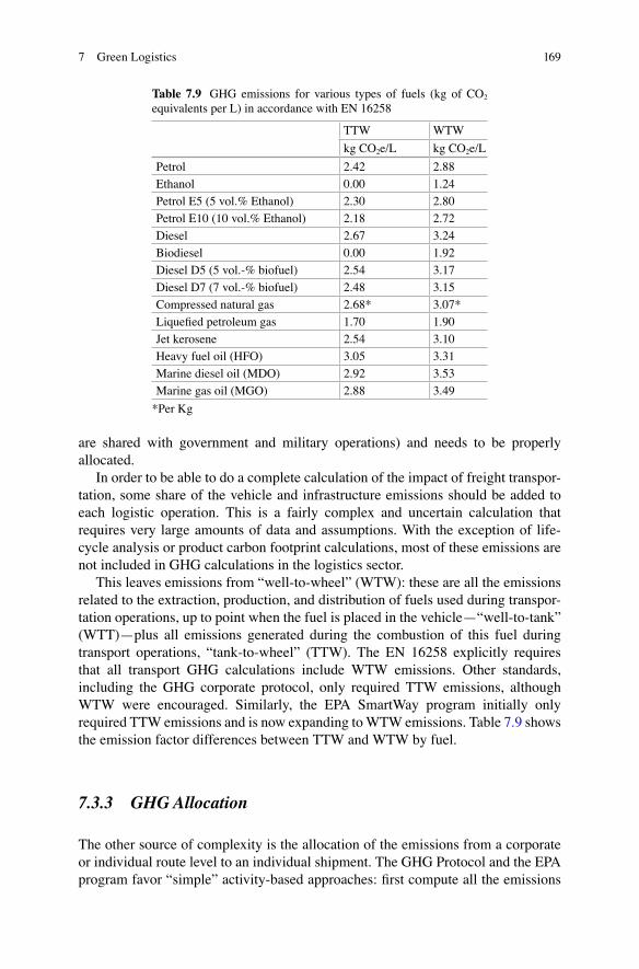
This leaves emissions from “well-to-wheel” (WTW): these are all the emissions related to the extraction, production, and distribution of fuels used during transpor-tation operations, up to point when the fuel is placed in the vehicle—“well-to-tank” (WTT)—plus all emissions generated during the combustion of this fuel during transport operations, “tank-to-wheel” (TTW). The EN 16258 explicitly requires that all transport GHG calculations include WTW emissions. Other standards, including the GHG corporate protocol, only required TTW emissions, although WTW were encouraged. Similarly, the EPA SmartWay program initially only required TTW emissions and is now expanding to WTW emissions. Table 7.9 shows the emission factor differences between TTW and WTW by fuel.

7.3.3 GHG Allocation

The other source of complexity is the allocation of the emissions from a corporate or individual route level to an individual shipment. The GHG Protocol and the EPA program favor “simple” activity-based approaches: first compute all the emissions

Table 7.9 GHG emissions for various types of fuels (kg of CO2 equivalents per L) in accordance with EN 16258

TTW WTW

kg CO2e/L kg CO2e/L

Petrol 2.42 2.88

Ethanol 0.00 1.24

Petrol E5 (5 vol.% Ethanol) 2.30 2.80

Petrol E10 (10 vol.% Ethanol) 2.18 2.72

Diesel 2.67 3.24

Biodiesel 0.00 1.92

Diesel D5 (5 vol.-% biofuel) 2.54 3.17

Diesel D7 (7 vol.-% biofuel) 2.48 3.15

Compressed natural gas 2.68* 3.07*

Liquefied petroleum gas 1.70 1.90

Jet kerosene 2.54 3.10

Heavy fuel oil (HFO) 3.05 3.31

Marine diesel oil (MDO) 2.92 3.53

Marine gas oil (MGO) 2.88 3.49

*Per Kg

7 Green Logistics

170

of a company or service using, for instance, fuel records. Then calculate the total distance (including empty miles) and weight moved during the transportation activ-ities. Once WTW or TTW emission factors are applied to fuel consumption data, they can be divided by the total ton-mile of the logistics or transportation provider to estimate an emission factor per ton-mile. This approach ignores the fact that indi-vidual routes or services may have different efficiency levels, or that specific vehi-cles may have different performance metrics, in favor of a simple and consistent calculation that can be easily adopted by many organizations. The EPA SmartWay program does allow for tracking emissions by type of fleet (e.g., flat bed trucks vs. drayage trucks), but it still recommends an aggregate approach for computing emis-sion factors.

The EN 16258, on the other hand, favors a detailed approach. It recommends using the product of the weight of the consignment and the actual distance trav-eled—i.e., the transport capacity measured in tonne kilometers—as the allocation parameter. It aims at providing as accurate as possible assignment of emission fac-tors to individual packages, taking into account logistics network configurations such as the relative location of the warehouse with respect to customers in a delivery route. Variations of this calculation are allowed in the standard, based on the quality of the information and type of service. An in-depth discussion of the EN 16258 standard is beyond this chapter, but this requires consistently collecting data across every transportation route, including shipment information, sequence, and distance. This is a gargantuan task, especially since logistics operations often include multi-ple providers with various levels of sophistication. Nevertheless, for large organiza-tions like UPS, DHL, FedEx, or Maersk, the EN 16258 does provide a framework to develop information systems that can provide very accurate shipment level- allocation of GHG emissions.

7.3.4 GHG Metric Trade-Offs

As discussed on this section, GHG Metrics will vary due to assumptions, scope, or data availability. Standards can guide organizations’ choices, but designing metrics that excel in all dimensions is not practically possible. Instead, firms must choose metrics that trade off between certain criteria. Two of the primary trade-offs are between integrative and useful metrics, and between robust and valid metrics (Caplice and Sheffi 1994) (Fig. 7.7).

Integrative metrics promote coordination across functions, while useful metrics are easily understood and provide managers with direct guidance. Providing managers with actionable guidance requires a level of specificity that makes pro-moting coordination across functions difficult. In this sense, measuring the carbon footprint of transportation is a useful metric, because it provides guidance on one specific aspect but not across functions. As such, it must be incorporated as one metric in an entire performance measurement system that covers both environmen-tal and non- environmental aspects across the functions of the supply chain.


171

The other trade-off is between a robust metric that allows for comparability and a valid metric that captures specific aspects. A valid metric, such as the ones favored by the EN16258, provides help with making a specific decision but is less suitable to external uses where it might be compared with similar metrics for other organiza-tions, unlike the GHG Protocol or EPA approaches.

7.4 Green Logistics Strategies

As discussed in the previous sections, logistics activities, though integral to the economic and social development, negatively impact the environment on multiple dimensions. The goal of green logistics is to mitigate the environmental impact of logistics—related activities.

As governments and companies have increased their focus on green logistics, numerous “best practices” and frameworks have been proposed (Craig et al. 2013). However, as the impacts outlined in the previous section show, there are five main logistics variables that, when combined, drive the environmental impact of logistics:

• Distance. How far are products being moved? Where are they loaded/unloaded?• Mode. Which mode of transportation is being used?• Equipment. What kind of equipment is being used for the logistics operation?

What kind of fuel and how much fuel does it consume?• Load. How much product is being loaded into the conveyance? How efficiently

is it loaded?• Operation. How skillful is the driver in operating the vehicle? How optimal is the

logistics plan?

Each of these variables is a lever that can be used toward designing greener logis-tics systems: distance reduction, modal shift, cleaner equipment, better load plan-ning, and operational excellence.

Promotes coordination

Captures specific aspects

Allows for comparability

Provides actionable guidance

Integrative

Useful Valid

Robust

Fig. 7.7 Trade-offs between criteria (Source: Caplice and Sheffi 1994)

7 Green Logistics

172

All business decisions, including logistics and transportation, are made at the strategic, tactical, or operational level (Stank and Goldsby 2000). Strategic deci-sions are revisited every 3–5 years, tactical decisions are often done with a 6-month to 2-year horizon in mind, and operational level decisions are made on a daily and weekly basis. Thus, decisions at strategic, tactical, and operational level are oppor-tunities to mitigate the environmental impact of logistics by flexing one or more of the five green logistics levers.

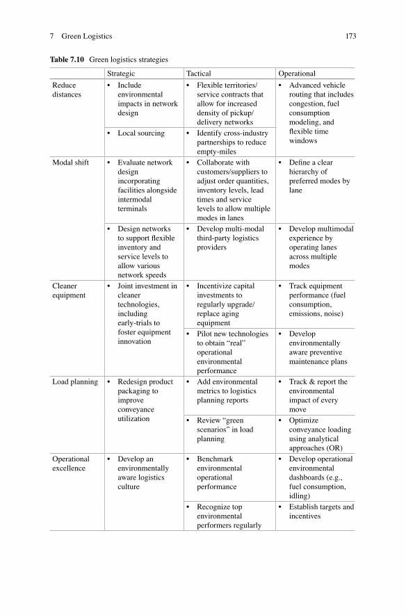
Table 7.10 shows a non-exhaustive list of green logistics strategies for each of the five levers across the three decision levels. These strategies require a combination of business and analytical approaches in logistics. Some of these strategies may appear simplistic or obvious, but they matter in practice. For instance, everyone recognizes that idling vehicles consumes fuel unnecessarily. According to the EPA SmartWay program, long-duration idling of truck and locomotive engines consumes more than 1 billion gallons of diesel fuel per year, emits 11 million tons of carbon dioxide, 200,000 t of oxides of nitrogen, 5000 t of particulate matter, and elevates noise lev-els (EPA 2015a). But only when there is a managerial commitment to reduce these impacts are the required actions taken, even when they are economically sound. Walmart, for examples, outfitted its 7000-vehicle truck fleet with auxiliary power units (APUs). Walmart estimated an 18-month payback period through fuel and engine wear savings, in addition to all associated environmental benefits.

The next two sections will expand on two well-studied modeling approaches—network design and vehicle-routing—that are commonly used in logistics decision- making and that have direct applicability on all levers at the strategic, tactical, and operational level. Business-centric dimensions will be further explored in the case studies of Sect. 7.4, focusing on real-life implementation challenges.

7.4.1 Network Design

Logistics network design is a strategic decision that has direct impact on two of the most important levers for green logistics: distance reduction and mode shift. It includes decisions related to the location of manufacturing plants, assembly facili-ties and multiple tiers of warehouses, as well as deciding how products flow through the network from suppliers to customers.

As elegantly summarized by Magnanti and Wong (1984), the basic ingredients of all network design models are a set of nodes (N) and a set of directed arcs (A) that are available to design the network. There are two types of decisions in network design models: (a) discrete-choice decisions relating to selecting which nodes and which arcs should be included in the final network and (b) decisions about the flow of one or multiple commodities from supply to demand nodes along the selected network. To find the optimal solution, mathematical models trade-off a variety of fixed and variable costs, as well as minimum and maximum flows, through each arc and node.


173

Table 7.10 Green logistics strategies

Strategic Tactical Operational

Reduce distances

• Includeenvironmental impacts in network design

• Flexibleterritories/service contracts that allow for increased density of pickup/delivery networks

• Advancedvehiclerouting that includes congestion, fuel consumption modeling, and flexible time windows

• Localsourcing • Identifycross-industrypartnerships to reduce empty-miles

Modal shift • Evaluatenetworkdesign incorporating facilities alongside intermodal terminals

• Collaboratewithcustomers/suppliers to adjust order quantities, inventory levels, lead times and service levels to allow multiple modes in lanes

• Defineaclearhierarchy of preferred modes by lane

• Designnetworksto support flexible inventory and service levels to allow various network speeds

• Developmulti-modalthird-party logistics providers

• Developmultimodalexperience by operating lanes across multiple modes

Cleaner equipment

• Jointinvestmentincleaner technologies, including early-trials to foster equipment innovation

• Incentivizecapitalinvestments to regularly upgrade/replace aging equipment

• Trackequipmentperformance (fuel consumption, emissions, noise)

• Pilotnewtechnologiesto obtain “real” operational environmental performance

• Developenvironmentally aware preventive maintenance plans

Load planning • Redesignproductpackaging to improve conveyance utilization

• Addenvironmentalmetrics to logistics planning reports

• Track&reporttheenvironmental impact of every move

• Review“greenscenarios” in load planning

• Optimizeconveyance loading using analytical approaches (OR)

Operational excellence

• Developanenvironmentally aware logistics culture

• Benchmarkenvironmental operational performance

• Developoperationalenvironmental dashboards (e.g., fuel consumption, idling)

• Recognizetopenvironmental performers regularly

• Establishtargetsandincentives

7 Green Logistics

174

Network design models are widely used and studied in logistics planning decisions, ranging from global flows (see Goetschalckx et al. 2002) to locating sin-gle facilities (see Melo et al. 2009). These models often include cost and service trade-offs.

Adding environmental considerations can be achieved by augmenting a tradi-tional network flow model with an environmental cost or an environmental constraint.

For instance, when deciding to open or close a facility in a network, there is often a fixed cost plus a variable cost driven by productivity, capacity, or labor choices. Because operating facilities may also generate environmental impacts that may vary by these same choices (e.g., pollution, GHG emissions), an “environmental cost” may be added to each candidate facility and then added as part of the objective func-tion to minimize total emissions or as constraint to limit the total environmental impacts (see Chap. 9 by Velázquez and Fransoo (2017)).

Another common variation to network flow models to take into account green impacts, is related to the flows through the network. Since every arc in the network represents the movement of one or more commodities via a mode of transportation, the model could explicitly estimate the environmental impact of this move using mode-specific emission factors. For example, Table 7.3 includes the amount of CO2 emitted per ton-mile for various modes. By multiplying these factors to the corre-sponding arc-flow variables, the model can estimate the total CO2 emissions of a particular transportation network configuration. These total transportation emis-sions could also be added to an objective function or part of a constraint to limit total emission costs. Because different transportation modes have different speeds, they will also have inventory impacts. To fully capture the network environmental impact, factors that measure the increased in emissions due to extra holding inven-tory may also be needed (e.g., extra energy required to hold extra inventory, extra waste generated due to increase obsolescence).

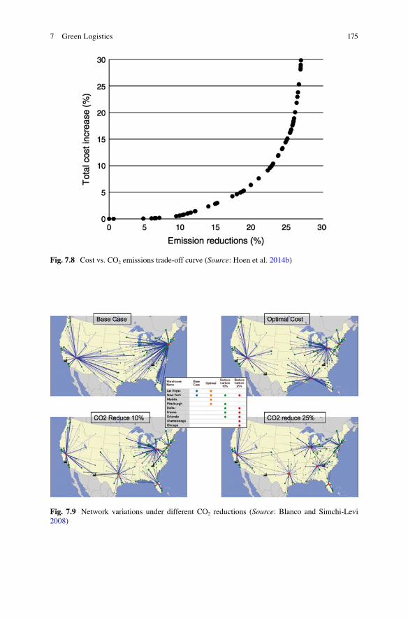
Hoen et al. (2014b) conducted a comprehensive modeling and analysis of the economic and environmental impact of selecting various transportation modes to fulfill customer orders for Cargill. They modeled the impact on revenue, inventory, and costs, and traded it off with total CO2 emissions. Figure 7.8 shows their results as a trade-off curve between reduction of emissions vs. cost increase.

Although the trade-off curve will vary depending on the specific network con-figuration, economics, and mode choices available, it often has a similar shape: it is possible to achieve noticeable environmental reductions without adding signifi-cant extra cost to the logistics network. In the case study analyzed by Hoen et al., 10 % CO2 reductions can be achieved by adding less than 1 % in cost. Achieving higher CO2 reductions (e.g., 25 %), however, will require a significant cost increase (e.g., 15 %).

In addition to the cost vs. environment trade-off analysis, analyzing various sce-narios can yield important insights to the network topology. Figure 7.9 shows the different network configurations for an apparel manufacturer in the USA under dif-ferent scenarios. In this case, the optimal cost scenario will open four warehouses,


175

Fig. 7.8 Cost vs. CO2 emissions trade-off curve (Source: Hoen et al. 2014b)

Fig. 7.9 Network variations under different CO2 reductions (Source: Blanco and Simchi-Levi 2008)

7 Green Logistics

176

compared to five or six facilities if the company would like to reduce 10 % and 25 % of total CO2 emissions in the network, respectively. More importantly, by looking at which facilities are selected under each scenario, logistics planners may elect to evaluate hybrid solutions that balance economic and environmental objectives.

7.4.2 Vehicle Routing

At the other end of the spectrum of network design is the daily execution of logistics activities. This includes warehouse operations (e.g., receiving, unloading, loading, storing, picking, and packing) and distribution operations (e.g., load building, prod-uct delivery, and product collection).

The design of the network and customer requirements limit the mode choices available for distribution operations, but there are still several levers that could be influenced directly, such as distance, equipment, and load building. Vehicle routing and scheduling is often the most environmentally intensive activity (from an energy and GHG perspective) because it is during the physical delivery of products that fuel is consumed and that the majority of transport emissions are generated (see Fig. 7.1).

There is a large body of literature devoted to solving vehicle routing problems (VRP) (see Laporte 2009 for a comprehensive review). These models almost always focus on minimizing distance, time, or cost of the planned routes. Although highly correlated, solving for minimum distance does not always translate into minimizing environmental impacts (Bektaş and Laporte 2011).

A similar approach to add environmental measurements to network design prob-lem, can be used to modify vehicle routing models: explicitly calculate the factors affecting fuel consumption and pollution such as equipment characteristics, cus-tomer time windows, product loaded during each leg of the route, speed of travel, slope of the road network, and congestion. These variations of VRP models are known as “pollution-routing problems” or PRP (Bektaş and Laporte 2011; Koç et al. 2014).

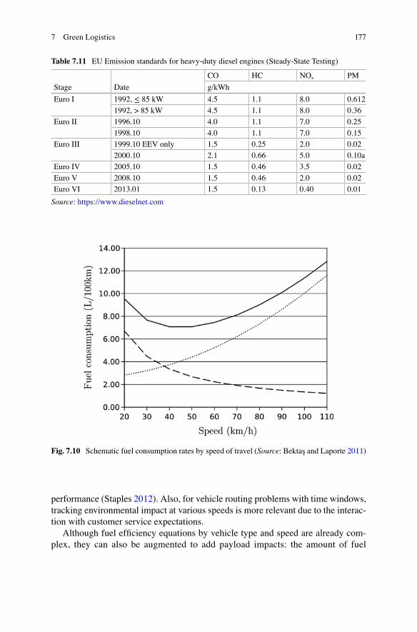
PRP problems explicitly capture the environmental impacts of vehicle routing operations. Assigning a vehicle to a route is one example. Besides differences in fuel consumption (that are part of the variable costs of operating a vehicle), dif-ferent types of vehicle technologies have different environmental impacts (see Table 7.11).

Speed of travel is another dimension of vehicle operations that is relevant in PRP problems. Figure 7.10 shows fuel consumption by speed for a light-weight vehicle. We can notice the U-shape of the curve leading to an optimal speed at 40 km/h. As vehicles are assigned to various road segments in a network with varying speeds, the total emissions generated may vary (e.g., highways or local roads). For instance, Staples was able to achieve an increase in fuel efficiency from 8.5 to 10.4 miles per gallon by limiting driver speeds to 60 miles per hour without impacting delivery


177

performance (Staples 2012). Also, for vehicle routing problems with time windows, tracking environmental impact at various speeds is more relevant due to the interac-tion with customer service expectations.

Although fuel efficiency equations by vehicle type and speed are already com-plex, they can also be augmented to add payload impacts: the amount of fuel

Table 7.11 EU Emission standards for heavy-duty diesel engines (Steady-State Testing)

Stage Date

CO HC NOx PM

g/kWh

Euro I 1992, ≤ 85 kW 4.5 1.1 8.0 0.612

1992, > 85 kW 4.5 1.1 8.0 0.36

Euro II 1996.10 4.0 1.1 7.0 0.25

1998.10 4.0 1.1 7.0 0.15

Euro III 1999.10 EEV only 1.5 0.25 2.0 0.02

2000.10 2.1 0.66 5.0 0.10a

Euro IV 2005.10 1.5 0.46 3.5 0.02

Euro V 2008.10 1.5 0.46 2.0 0.02

Euro VI 2013.01 1.5 0.13 0.40 0.01

Source: https://www.dieselnet.com

Fig. 7.10 Schematic fuel consumption rates by speed of travel (Source: Bektaş and Laporte 2011)

7 Green Logistics

178

consumed while traveling at a certain speed increases with the amount of cargo hauled (Barth and Boriboonsomsin 2009). Thus, it is theoretically possible to reduce environmental impacts on vehicle routes by giving priority to deliver large payloads early in the route, due to the potential to continue the route with a lighter load. Furthermore, by modeling road slopes or stop lights, one can further explore route variations that can further reduce fuel consumption and emissions. UPS delivery routes, for example, are designed to minimize left turns, which require vehicles to wait at an intersection for traffic to clear before making the turn. UPS has lowered CO2 emissions by 100,000 metric tons (UPS 2015).

7.5 Case Studies: Implementing Green Logistics Strategies

The strategies included in Table 7.10 are known to reduce emissions and, in some cases, also drive cost savings. Nevertheless, companies often have trouble imple-menting them.

One of the challenges is focus: these initiatives are not always management priority. Another key obstacle is that they require internal and external collabora-tion. The logistics function interfaces with multiple business activities and supports a wide range of decisions. Client-supplier relationships, outsourcing arrangements, cost sharing, and coordination between trading partners are a few examples.

The following four case studies illustrate how, through collaboration, green logistics initiatives were put into practice.2 The case studies focus on some of the unique business considerations and details required to make green logistics success-ful in practice. The first case study discusses how Boise was able to shift from truck to rail shipments and increase its load utilization by working with its customers on service and inventory impacts and through internal improvements of package design. The second case study also discusses modal shift, but this time achieved by two competitors sharing “empty miles” of a rail backhaul leg. The third case study is an example of a package redesign in Caterpillar’s inbound network that that reduces shipment weight and thus consumes less transportation fuel. The section concludes by describing the EPA SmartWay program, a multi-stakeholder voluntary collaboration that has incentivized companies to prioritize green logistics efforts by providing the right incentives and transparency to the process.

2 The first three cases studies in this section closely follow “Delivering on the Promise of Green Logistics,” by Edgar Blanco and Ken Cotrill (Blanco and Cottrill 2013).


179

7.5.1 Customer Collaboration: OfficeMax and Boise, Inc.

Boise, Inc. manufactures a wide range of packaging and paper products, with reported earnings of $2.56 billion in 2012.3 The company operates mainly in the USA and has long-term relationships with many customers, including retailer OfficeMax. Boise supplies the majority of OfficeMax’s paper products due to a long tradition of business and commercial relationships.

Truck transportation offers Boise the flexibility and speed it needs to meet cus-tomer delivery promises. However, moving products by truck also accounts for the largest percentage of the CO2 emissions associated with logistics operations. Rail transport is more cost effective and emits much less carbon per equivalent weight and distance, but it’s also slower and less flexible than trucking.

As part of its cost and environmental efforts, Boise developed two initiatives. In the first one, called Carload Direct, Boise needed to coordinate with its long-time partner OfficeMax. Prior to the initiative, shipments from Boise were routinely moved by truck to the retailer’s facilities, even when the destinations were accessi-ble by rail. OfficeMax became a test case for switching to direct-by-rail shipments. The two companies’ longstanding relationship helped Boise negotiate the change, but the Boise team was still tasked to make sure the transition did not disrupt OfficeMax’s ordering process.

The benefits of the change, carbon-wise, were significant: a traditional truckload shipment comprises about 20 t of paper product, whereas a railcar carries around 70 t. The main drawback to the process is that a rail solution required customer orders to be warehoused until there was enough freight to fill a boxcar. This meant that the time from order placement to delivery was potentially extended, while run-ning the risk that inventory needed by stores would be stuck in a warehouse. By coordinating the ordering process, the Boise team was able to determine when enough OfficeMax orders were available to “pool” into a Carload Direct shipment or when a regular truck shipment was the best option.

The solution may seem straightforward, but it required extensive cooperation between the transportation departments at Boise and OfficeMax. For example, ordering processes had to be adjusted and coordinated to take account of the change in product flows. Not every SKU was suitable for a Carload Direct shipment, so the teams had to select products that could be part of the pooling system. And the changes had to be made without altering the inventory positions or service levels of either enterprise, especially OfficeMax. The shift from using a mix of truck and rail to primarily rail between the major Boise and OfficeMax distribution centers elimi-nated more than 2600 t of CO2, a 70 % reduction compared to truckload shipments, or the equivalent of saving over 264,000 gal of fuel consumed by road vehicles.

3 The Boise organization described in this case study refers to Boise Cascade LLC, the paper and forest products. It should not be confused with Boise Cascade Corporation that is now OfficeMax Incorporated.

7 Green Logistics

180

Both companies benefitted from this greener supply chain as the reduced transporta-tion costs were shared between them.

For the second initiative, Boise looked at its packaging and loading processes. Paper products are often ordered in large quantities and shipped in full pallets. Boise field operations noticed that full pallets did not always maximize the space in the rail boxcars. Boise redesigned its pallets and loading procedures to accommodate a half-pallet, which allowed Boise to reorganize pallet stacking and maximize ship-ping capacities for its loads. Once the operational configuration was solved, Boise needed to work with its customers to allow orders that included a half-pallet size.

Boise created new SKUs and modified ordering and receiving systems to allow for the new half-pallet product configuration. The company realized that this was a win-win situation; the half-pallet solution was a perfect fit for companies that shipped seasonal and low-demand products. Using just 930 railcars in 2011, Boise reduced the company’s CO2 emissions by 190 t or 6.8 % of its annual rail shipment emissions without any extra cost. This is equal to the CO2 emissions from 21,600 gal of fuel, or the annual GHG emissions from 38 passenger vehicles. In addition to improving the environmental performance of Boise and participating customers, the smaller, the half-pallet unit gave Boise and its customers more order flexibility.

7.5.2 Competitor Collaboration: Ocean Spray and Tropicana

Identifying opportunities for using intermodal can be challenging. The respective transportation services must mesh seamlessly in order to maintain service standards and avoid delays that could result in the costly build-up of inventory. Ocean Spray captured such an opportunity in an unconventional way: it collaborated with a competitor.

Ocean Spray is an agricultural cooperative owned by more than 700 cranberry growers in Massachusetts, Wisconsin, New Jersey, Oregon, Washington, Canada, and Chile, as well as 35 Florida grapefruit growers. The organization posted fiscal 2012 gross sales of $2.2 billion and net proceeds of $338 million.

One of Ocean Sprays’ most significant logistics expenses—and a major con-tributor to its carbon footprint—was the need to ship product from its Bordentown, New Jersey, distribution center over 1000 miles to another distribution center in Lakeland, Florida. By coincidence, both of these distribution centers were located a short distance (60–65 miles) from rail yards used by a competitor, Tropicana, which shipped orange juice north from Florida in special refrigerated boxcars.

Tropicana also had a key difficulty when it came to logistics. Although it could send product direct from Florida up to the CSX rail terminal in New Jersey, once offloaded, the refrigerated rail boxcars were often traveling empty back to Florida.

Tropicana’s third-party logistics (3PL) provider, Wheels Clipper, saw an oppor-tunity to help its client while earning the trust of a new customer. The company approached Ocean Spray and proposed that they operate an intermodal lane from New Jersey to Florida that would put Tropicana’s empty orange juice boxcars to use


181

on Ocean Spray’s behalf. The goal was to save Ocean Spray money (and reduce emissions) by allowing them to switch from trucking their cranberry juice to send-ing it more efficiently by rail, while also saving Tropicana the cost and emissions associated with empty cars returning south.

The plan provided environmental benefits and lowered costs for both companies. But there were potential downsides. To make the idea work, Ocean Spray would have to switch logistics providers and work with a new 3PL, transporting via a mode with which the company was unfamiliar. Even more challenging, the arrangement required Ocean Spray to collaborate with one of the company’s strongest competi-tors in the beverage business, Tropicana.

Using the intermodal solution would save Ocean Spray over 40 % in transporta-tion costs compared to the previous trucking method, and it would also reduce its GHG emissions by a 65 %. Meanwhile, Tropicana would eliminate most of the costs and GHG emissions of the boxcars’ return trip from its ledger—a significant reduc-tion in each metric, at the price of some (admittedly complex) process changes.

Ocean Spray accepted that the plan did make sense, and the company reconfig-ured its load planning processes to make shipments compatible with the rail mode. Tropicana and Wheels Clipper also needed to change their operating procedures to communicate railcar availability to Ocean Spray. To guarantee the on-time delivery of all shipments, all the participants worked to improve supply chain visibility. For example, they improved the flow of information between the parties on the status of shipments and potential delays. As the intermediary, Wheels Clipper helped to ensure that this information was delivered to the relevant parties in a timely fashion.

During several pilot runs, the companies were able to coordinate load pickup and delivery within required time windows, and to confirm that product was being han-dled properly. The trials also revealed potential problems. For example, the new intermodal solution added 1–2 days to transit times, and Ocean Spray had to adjust its logistics operations to avoid having a negative impact on customer service. Yet in the end, the fact that there was a clear ROI for both shippers gave incentives to the participants that helped them to move the project forward and make it successful.

7.5.3 Supplier Collaboration: Caterpillar and Part Suppliers

Caterpillar Global Mining Division makes specialized trucks for the mining indus-try. Over the past 30 years, Caterpillar has produced nearly three times as many trucks as its closest competitor. The company assembled its 50,000th rigid-frame construction and mining truck in 2009.

Caterpillar worked on an initiative focused on the North American inbound parts logistics for Caterpillar’s manufacturing facility in Decatur, Illinois. The goal was to reduce the weight of the thousands of returnable packing containers that Caterpillar used to transport parts from suppliers. Replacing the heavy metal packing containers

7 Green Logistics

182

with light-weight plastic units cuts the weight of shipments, which translates into less fuel consumption and reduced carbon emissions.

However, the effort required Caterpillar to coordinate with multiple suppliers in different countries. It was a daunting challenge, particularly when long-established practices have to be changed. Some of these containers had been in circulation for more than 50 years.

Prior to the carbon footprint study, Caterpillar’s internal analysis had determined that the fuel savings from light-weighting inbound containers would be significant. Yet Caterpillar had been slow to adopt the plastic containers because of several internal organizational and budgetary constraints.

The first step was to carry out a detailed analysis of the inbound flow of contain-ers. In partnership with MIT, Caterpillar analyzed 16 weeks of transportation data that included detailed information about North American suppliers, number of parts shipped, and delivery dates for three of the flagship mining trucks. The data included more than 15,000 truck deliveries of 1400 different item numbers from more than 200 suppliers that ship directly to the Decatur manufacturing plant. The Caterpillar and MIT teams determined that 9.5 % of shipments were eligible for light-weight packaging.

By reducing the shipping containers from 130 to 200 lb each to 20–40 lb each, Caterpillar could reduce CO2 emissions across the Caterpillar North American net-work by 130 t. Caterpillar could now present a strong environmental case, in addi-tion to a 2-year ROI viable financial benefit to all internal and external stakeholders affected by the packaging changes.

7.5.4 The EPA SmartWay Program

The SmartWay Transport Partnership is an innovative voluntary collaborative pro-gram between the EPA and the freight industry designed to improve energy effi-ciency and to lower GHG emissions and air pollution. Started in February 2004, the partnership aims to create strong market-based incentives for companies shipping products, and for the truck and rail companies delivering those products, to improve the environmental performance of their freight operations.

7.5.4.1 History4

In 2003, staff at the EPA’s Office of Transportation and Air Quality (OTAQ) devel-oped an initial concept to build an innovative voluntary freight transportation pro-gram focused on energy savings and emission reductions. They worked for over a

4 Based on interviews and research conducted by K. C. Tan and E. E. Blanco from the MIT Center for Transportation & Logistics in 2009.


183

year in collaboration with a group of public and private stakeholders to develop the foundation of the EPA SmartWay Transport Partnership. Members of the group included the American Trucking Association, Business for Social Responsibility, Canon USA, Coca Cola Enterprises, CSX, FedEx, H-E-B Grocery, Home Depot, IKEA, Interface, Nike, Norm Thompson Outfitters, Schneider National, Swift Transportation, UPS, and YRC Worldwide.

Together, these stakeholders and the EPA designed a freight transportation pro-gram that addressed the goals and needs of both the freight industry and the EPA. The freight industry was interested in an improved public image, recognition for its efforts, and fuel savings to help companies in an extremely competitive industry. The EPA was interested in reducing emissions from diesel engines and improving energy security in the freight industry. The companies provided critical operational and technical insight into freight management and supply chain logis-tics. Their input helped the EPA to identify appropriate fuel saving technologies for heavy trucks and to develop a fuel and emissions tracking tool that carriers and shippers could use to track their performance.

Because program enrollment was going to be on a voluntary basis, it was impor-tant to make it attractive for companies to participate and to motivate them toward a collaborative solution in addressing energy and environmental issues in the freight sector. After much planning, the EPA formally launched the program with the full support of the trucking industry at the American Trucking Association’s annual conference on February 9, 2004, with 15 initial charter partners.

7.5.4.2 Program Structure

The SmartWay Transport Partnership is tailored to progressive corporations and organizations involved in shipping goods. Companies that provide and hire freight delivery services become SmartWay Transport Partners by committing to improve the environmental performance of their freight delivery operations. SmartWay Transport Carriers commit to integrate innovative cost saving strategies into their fleet operations. SmartWay Transport Shippers commit to ship the majority of their goods with SmartWay Transport Carriers. Companies that meet SmartWay Transport Partnership requirements benefit from reduced operating costs and enhanced recog-nition and visibility: partners that demonstrate superior performance earn the right to display the SmartWay Transport logo.

The SmartWay program also provides technical assistance to help partners benchmark and evaluate the effectiveness of a broad range of technology, equip-ment controls, and fuel-saving logistics management strategies. The SmartWay pro-gram has also established connections with financial institutions to provide flexible, reduced-interest loans to improve access to these fuel-saving technologies and pol-lution controls.

7 Green Logistics

184

7.5.4.3 Impact

Since 2004, SmartWay partners have eliminated over 51 million metric tons of CO2, saved over 120 million barrels of oil and $16 billion in fuel costs, and reduced 738,000 t of NOx and 37,000 t of PM (EPA 2014).

The success of SmartWay in the USA has led to its adoption in Canada, where Natural Resources Canada now administers the program for Canadian firms, using the same tools methods and metrics for assessing freight efficiency. In addition, the SmartWay public–private partnership model is now being replicated in other coun-tries in Latin America, Asia, and the European Union. SmartWay is also being used as a template to inform the development of freight sustainability programs under the United Nations Climate Environment Program’s and Clean Air Coalition (EPA 2014).

7.6 Beyond Green Logistics

This chapter has presented various levers available to improve the environmental impact of logistics operations. Most of the approaches discussed are familiar to logisticians: optimize distance, maximize loads, assign the right equipment and resource, and avoid waste. These are themes that have been used for many years to reduce cost and improve service. The same systematic approach can be used to make logistics better for the environment.

Underlying all the success stories and approaches presented throughout the chapter—from network design, vehicle routing or multi-stakeholder collabora-tion—is the need for a solid measurement foundation of GHG, pollution, noise, and waste impacts. Unlike financial measurements that are common and well under-stood, environmental metrics are uncertain and continuously evolving. Green logis-tics is not only about finding the optimal solution to an environmental metric, but also to make sure that traditional strategies are reviewed with environmental lenses. New trade-offs may be uncovered, as well as new sources of value and cost reduction.

This chapter uses a narrow scope—just logistics activities—for all analyses of impacts and strategies for improving. In transport sustainability some cases, a broader scope of analysis, such as an end-to-end life-cycle analysis, will reveal trade-offs between the greenest choices in logistics and greenest choices in sourc-ing, manufacturing, returns, product design, and so forth. For example, differences in manufacturing efficiencies or the energy portfolios of different regions may mean that higher impacts in transportation permit much lower environmental impacts overall. Or, a slower mode of transport might reduce transportation emissions but increase the amount of waste due to spoilage, obsolescence, or excessive inventory.


185

Thus, the analyses and strategies in this chapter are an element of a broader process of analyzing and improving the sustainability of the business or supply chain at a more holistic level. As a consequence, there are more opportunities related to green logistics. Reverse logistics and closed loop supply chains (see Chap. 17 by Abbey and Guide (2017)) adds a new dimension to managing waste by focusing on how to recover products delivered to customers and extract new sources of value. Technological improvements that completely avoid emissions, such as solar energy, could completely avoid the need to reconfigure logistics net-works. Advances in nanomaterials and biodegradable materials may make packag-ing waste a nonissue. And, in some cases, life-cycle thinking may challenge logistics operations to increase their impact to allow for a holistic reduction of the environmental impact of products: it may be sometimes better to import a product from the other side of the world if energy sources are cleaner there than to manu-facture it locally.

A new generation of green logistics choices is quickly unfolding, and the con-cepts discussed in this chapter provide a foundation for the journey ahead.

References

Abbey JD, Guide VDR Jr (2017) Closed-loop supply chains: a strategic overview. In: Bouchery Y, Corbett CJ, Fransoo J, Tan T (eds) Sustainable supply chains: a research-based textbook on operations and strategy. Springer, New York

Barth M, Boriboonsomsin K (2009) Energy and emissions impacts of a freeway-based dynamic eco-driving system. Transp Res Part D: Transp Environ 14(6):400–410

Bektaş T, Laporte G (2011) The pollution-routing problem. Transp Res B Methodol 45(8):1232–1250

Blanco E, Cottrill K (2013) Delivering on the promise of green logistics. MIT Sloan Manag Rev. http://sloanreview.mit.edu/article/delivering-on-the-promise-of-green-logistics/. Accessed 16 Dec 2013

Blanco E, Simchi-Levi D (2008). Generating a sustainability scorecard: assessing your company’s footprint. CSCMP annual conference

Boukherroub T, Bouchery Y, Corbett CJ, Fransoo J, Tan T (2017) Carbon footprinting in supply chains. In: Bouchery Y, Corbett CJ, Fransoo J, Tan T (eds) Sustainable supply chains: a research-based textbook on operations and strategy. Springer, New York

Caplice C, Sheffi Y (1994) A review and evaluation of logistics metrics. Int J Logist Manag 5(2):11–28

Carslaw D, et al. (2011) Trends in NOx and NO2 emissions and ambient measurements in the UK. DEFRA, London

Craig A.J., Blanco E.E., Caplice C.G. (2013). “Carbon Footprint of Supply Chains: A Scoping Study”. Final Report for NCFRP Project 36 (04).

EPA (2014) Mobile source technical review subcommittee: SmartWay Legacy Fleet Workgroup. Recommendations and findings

EPA (2015a) SmartWay Technology. http://epa.gov/smartway/forpartners/technology.htmEPA (2015b). Municipal solid waste generation, recycling, and disposal in the United States: facts

and figures for 2010 (pp 1–12)European Environmental Agency (2015). Emissions of air pollutants from transport. http://www.

eea.europa.eu/data-and-maps/indicators/transport-emissions-of-air-pollutants-8/transport- emissions- of-air-pollutants-2

7 Green Logistics

186

Forkenbrock DJ (1999) External costs of intercity truck freight transportation. Transp Res A Policy Pract 33(7):505–526

Goetschalckx M, Vidal CJ, Dogan K (2002) Modeling and design of global logistics systems: a review of integrated strategic and tactical models and design algorithms. Eur J Oper Res 143(1):1–18

Greene DL, Plotkin SE (2011) Reducing greenhouse gas emissions from US Transportation. Pew Center on Global Climate Change, Arlington

Hoen KMR, Tan T, Fransoo JC, van Houtum GJ (2014a) Effect of carbon emission regulations on transport mode selection under stochastic demand. Flex Serv Manuf J 26(1–2):170–195

Hoen KMR, Tan T, Fransoo JC, van Houtum GJ (2014b) Switching transport modes to meet vol-untary carbon emission targets. Transp Sci 48(4):592–608

IEA (2009) Transport, energy and CO2. Technical report. OECD, ParisIMO (2009) Second IMO GHG Study 2009. International Maritime Organization (IMO), LondonIMO (2012). International shipping facts and figures. International Maritime OrganizationIMO (2015). Introduction to the IMO. http://www.imo.or. Accessed Nov 2015IPCC (2006). IPCC guidelines for national greenhouse gas inventories. In: Eggleston S, Buendia

L, Miwa K, Ngara T, Tanabe K. IGES, JapanKoç Ç et al (2014) The fleet size and mix pollution–routing problem. Transp Res B Methodol

70:239–254Laporte G (2009) Fifty years of vehicle routing. Transp Sci 43(4):408–416Liedtke G and Friedrich H (2012) Generation of logistics networks in freight transportation mod-

els. Transportation: 1–17Magnanti TL, Wong RT (1984) Network design and transportation planning: models and algo-

rithms. Transp Sci 18(1):1–55Martin S and Wolfram K (2012) Calculating GHG emissions for freight forwarding and logistics

services. European Association for Forwarding, Transport, Logistics and Customs Services (CLECAT)

Mathers J et al (2014) The green freight handbook. Environmental Defense FundMelo MT, Nickel S, Saldanha-da-Gama F (2009) Facility location and supply chain management–

a review. Eur J Oper Res 196(2):401–412NTM (2010). Road transport Europe. Network for Transport and EnvironmentNew York City Department of Environmental Protection - NYCDEP (2008). A guide to New York

City’s Noise Code. http://www.nyc.gov/html/dep/pdf/noise_code_guide.pdf Paine F (2002) Packaging reminiscences: some thoughts on controversial matters. Packag Technol Sci 15(4):167–179

Richter A et al (2004) Satellite measurements of NO2 from international shipping emissions. Geophys Res Lett 31(23)

Saphire D (1994) Delivering the goods: benefits of reusable shipping containers. INFORM, New York

Sheffi Y, Daganzo C (1978) Hypernetworks and supply-demand equilibrium obtained with disag-gregate demand models. Transp Res Rec 673

Soroka W (1999) Fundamentals of packaging technology, Vol 3. Institute of Packaging Professionals

Stank TP, Goldsby TJ (2000) A framework for transportation decision making in an integrated supply chain. Supply Chain Manag Int J 5(2):71–78

Staples (2012) Interview to Mike Payette. http://www.brightfleet.com/blog/2012/interview - with- mike-payette-at-staples-about-speed-limiters-fuel-economy-and-safety/

UPS Pressroom. https://www.pressroom.ups.com/pressroom/ContentDetailsViewer.page?Concept Type = FactSheets&id=1426321581228-233. Accessed 2015

Velázquez Martínez JC, Fransoo JC (2017) Green facility location. In: Bouchery Y, Corbett CJ, Fransoo J, Tan T (eds) Sustainable supply chains: a research-based textbook on operations and strategy. Springer, New York


187

VTT Technical Research Centre of Finland (2012). Methodologies for emission calculations—best practices, implications and future needs. COFRET

Wang H, Liu D, Dai G (2009) Review of maritime transportation air emission pollution and policy analysis. J Ocean Univ China 8(3):283–290

Winebrake JJ, Corbett JJ et al (2008) Assessing energy, environmental, and economic tradeoffs in intermodal freight transportation. J Air Waste Manage Assoc 58(8):1004–1013

World Economic Forum—WEF (2009) Supply chain decarbonization (pp 1–41)Zamboni G et al (2015) Experimental evaluation of Heavy Duty Vehicle speed patterns in urban

and port areas and estimation of their fuel consumption and exhaust emissions. Transp Res D Transp Environ 35:1–10

7 Green Logistics

Chapter 7 Green Logistics - Home | Professor Yossi …...Green Logistics Edgar E. Blanco and Yossi...

Documents

Transcript of Chapter 7 Green Logistics - Home | Professor Yossi …...Green Logistics Edgar E. Blanco and Yossi...