Chapter 7. Electromagnetic Wave Propagation
68
Essential Graduate Physics EM: Classical Electrodynamics © K. Likharev Chapter 7. Electromagnetic Wave Propagation This (rather extensive) chapter focuses on the most important effect that follows from the time- dependent Maxwell equations, namely the electromagnetic waves, at this stage avoiding a discussion of their origin, i.e. the radiation process – which will the subject of Chapters 8 and 10. The discussion starts from the simplest, plane waves in uniform and isotropic media, and then proceeds to non-uniform systems, bringing up such effects as reflection and refraction. Then we will discuss the so-called guided waves, propagating along various long transmission lines – such as coaxial cables, waveguides, and optical fibers. Finally, the end of the chapter is devoted to final-length fragments of such lines, serving as resonators, and to effects of energy dissipation in transmission lines and resonators. 7.1. Plane waves Let us start from considering a spatial region that does not contain field sources ( = 0, j = 0), and is filled with a linear, uniform, isotropic medium, which obeys Eqs. (3.46) and (5.110): H B E D , . (7.1) Moreover, let us assume for a while, that these constitutive equations hold for all frequencies of interest. (Of course, these relations are exactly valid for the very important particular case of free space, where we may formally use the macroscopic Maxwell equations (6.100), but with = 0 and = 0 .) As was already shown in Sec. 6.8, in this case, the Lorenz gauge condition (6.117) allows the Maxwell equations to be recast into the wave equations (6.118) for the scalar and vector potentials. However, for most purposes, it is more convenient to use the homogeneous Maxwell equations (6.100) for the electric and magnetic fields – which are independent of the gauge choice. After an elementary elimination of D and B using Eqs. (1), 1 these equations take a simple, very symmetric form: , 0 t H E , 0 t E H (7.2a) , 0 E . 0 H (7.2b) Now, acting by operator on each of Eqs. (2a), i.e. taking their curl, and then using the vector algebra identity (5.31), whose first term, for both E and H, vanishes due to Eqs. (2b), we get fully similar wave equations for the electric and magnetic fields: 2 , 0 1 , 0 1 2 2 2 2 2 2 2 2 H E t v t v (7.3) 1 Though B rather than H is the actual magnetic field, mathematically it is a bit more convenient (just as it was in Sec. 6.2) to use the vector pair {E, H} in the following discussion, because at sharp media boundaries, it is H that obeys the boundary condition (5.117) similar to that for E – cf. Eq. (3.37). 2 The two vector equations (3) are of course is just a shorthand for six similar equations for three Cartesian components of E and H, and hence for their magnitudes E and H. where the parameter v is defined as Maxwell equations for uniform linear media EM wave equations
Transcript of Chapter 7. Electromagnetic Wave Propagation

Essential Graduate Physics EM: Classical Electrodynamics
© K. Likharev
Chapter 7. Electromagnetic Wave Propagation
This (rather extensive) chapter focuses on the most important effect that follows from the time-dependent Maxwell equations, namely the electromagnetic waves, at this stage avoiding a discussion of their origin, i.e. the radiation process – which will the subject of Chapters 8 and 10. The discussion starts from the simplest, plane waves in uniform and isotropic media, and then proceeds to non-uniform systems, bringing up such effects as reflection and refraction. Then we will discuss the so-called guided waves, propagating along various long transmission lines – such as coaxial cables, waveguides, and optical fibers. Finally, the end of the chapter is devoted to final-length fragments of such lines, serving as resonators, and to effects of energy dissipation in transmission lines and resonators.
7.1. Plane waves
Let us start from considering a spatial region that does not contain field sources ( = 0, j = 0), and is filled with a linear, uniform, isotropic medium, which obeys Eqs. (3.46) and (5.110):
HBED , . (7.1)
Moreover, let us assume for a while, that these constitutive equations hold for all frequencies of interest. (Of course, these relations are exactly valid for the very important particular case of free space, where we may formally use the macroscopic Maxwell equations (6.100), but with = 0 and = 0.) As was already shown in Sec. 6.8, in this case, the Lorenz gauge condition (6.117) allows the Maxwell equations to be recast into the wave equations (6.118) for the scalar and vector potentials. However, for most purposes, it is more convenient to use the homogeneous Maxwell equations (6.100) for the electric and magnetic fields – which are independent of the gauge choice. After an elementary elimination of D and B using Eqs. (1),1 these equations take a simple, very symmetric form:
,0
t
HE ,0
t
EH (7.2a)
,0E .0H (7.2b)
Now, acting by operator on each of Eqs. (2a), i.e. taking their curl, and then using the vector algebra identity (5.31), whose first term, for both E and H, vanishes due to Eqs. (2b), we get fully similar wave equations for the electric and magnetic fields:2
,01
,01
2
2
22
2
2
22
HEtvtv
(7.3)
1 Though B rather than H is the actual magnetic field, mathematically it is a bit more convenient (just as it was in Sec. 6.2) to use the vector pair {E, H} in the following discussion, because at sharp media boundaries, it is H that obeys the boundary condition (5.117) similar to that for E – cf. Eq. (3.37). 2 The two vector equations (3) are of course is just a shorthand for six similar equations for three Cartesian components of E and H, and hence for their magnitudes E and H.
where the parameter v is defined as
Maxwell equations
for uniform linear
media
EM wave equations

Essential Graduate Physics EM: Classical Electrodynamics
Chapter 7 Page 2 of 68
12 v . (7.4)
with v2 = 1/00 c2 in free space – see Eq. (6.120) again.
These equations allow, in particular, solutions of the following particular type;
),( vtzfHE (7.5)
where z is the Cartesian coordinate along a certain (arbitrary) direction n, and f is an arbitrary function of one argument. This solution describes a specific type of a traveling wave – meaning a certain field pattern moving, without deformation, along the z-axis, with velocity v. According to Eq. (5), both E and H have the same values at all points of each plane perpendicular to the direction n nz of the wave propagation; hence the name – plane wave.
According to Eqs. (2), the independence of the wave equations (3) for vectors E and H does not mean that their plane-wave solutions are independent. Indeed, plugging any solution of the type (5) into Eqs. (2a), we get
nHEEn
H
ZZ
i.e., , (7.6)
where
2/1
H
EZ . (7.7)
The vector relationship (6) means, first of all, that the vectors E and H are perpendicular not only to the propagation vector n (such waves are called transverse), but also to each other (Fig. 1) – at any point of space and at any time instant. Second, this equality does not depend on the function f, meaning that the electric and magnetic fields increase and decrease simultaneously.
Finally, the field magnitudes are related by the constant Z, called the wave impedance of the medium. Very soon we will see that the impedance plays a pivotal role in many problems, in particular at the wave reflection from the interface between two media. Since the dimensionality of E, in SI units, is V/m, and that of H is A/m, Eq. (7) shows that Z has the dimensionality of V/A, i.e. ohms ().3 In particular, in free space,
3 In the Gaussian units, E and H have a similar dimensionality (in particular, in a free-space wave, E = H), making the (very useful) notion of the wave impedance less manifestly exposed – so that in some older physics textbooks it is not mentioned at all!
E
k
H0 Fig. 7.1. Field vectors in a plane electromagnetic wave propagating along direction n.
n
Wave velocity
Field vector relationship
Wave impedance
Plane wave

Essential Graduate Physics EM: Classical Electrodynamics
Chapter 7 Page 3 of 68
Ω377104 7
2/1
0
00
cZZ
. (7.8)
Next, plugging Eq. (6) into Eqs. (6.113) and (6.114), we get:
22 HEu , (7.9a)
,22
ZHZ
EnnHES (7.9b)
so that, according to Eqs. (4) and (7), the wave’s energy and power densities are universally related as
uvnS . (7.9c)
In the view of the Poynting vector paradox discussed in Sec. 6.8 (see Fig. 6.11), one may wonder whether the last equality may be interpreted as the actual density of power flow. In contrast to the static situation shown in Fig. 6.11, which limits the electric and magnetic fields to vicinity of their sources, waves may travel far from them. As a result, they can form wave packets of a finite length in free space – see Fig. 2.
Let us apply the Poynting theorem (6.111) to the cylinder shown with dashed lines in Fig. 2, with one lid inside the wave packet, and another lid in the region already passed by the wave. Then, according to Eq. (6.111), the rate of change of the full field energy E inside the volume is dE /dt = –SA (where A is the lid area), so that S may be indeed interpreted as the power flow (per unit area) from the volume. Making a reasonable assumption that the finite length of a sufficiently long wave packet does not affect the physics inside it, we may indeed interpret the S given by Eqs. (9b-c) as the power flow density inside a plane electromagnetic wave.
As we will see later in this chapter, the free-space value Z0 of the wave impedance, given by Eq. (8), establishes the scale of Z of virtually all wave transmission lines, so we may use it, together with Eq. (9), to get a better feeling of how much different are the electric and magnetic field amplitudes in the waves – on the scale of typical electrostatics and magnetostatics experiments. For example, according to Eqs. (9), a wave of a modest intensity S = 1 W/m2 (this is what we get from a usual electric bulb a few meters away from it) has E ~ (SZ0)
1/2 ~ 20 V/m, quite comparable with the dc field created by a standard AA battery right outside it. On the other hand, the wave’s magnetic field H = (S/Z0)
1/2 0.05 A/m. For this particular case, the relation following from Eqs. (1), (4), and (7),
n
Fig. 7.2. Interpreting the Poynting vector in a plane electromagnetic wave. (Horizontal lines show equal-field planes.)
0S
0S
packet wave
V
Wave’s energy
Wave impedance
of free space
Wave’s power
Essential Graduate Physics EM: Classical Electrodynamics
Chapter 7 Page 4 of 68
v
EE
E
Z
EHB 2/1
2/1/
, (7.10)
gives B = 0H = E/c ~ 710-8T, i.e. a magnetic field a thousand times lower than the Earth’s field, and about 7 orders of magnitude lower than the field of a typical permanent magnet. This huge difference may be interpreted as follows: the scale of magnetic fields B ~ E/c in the waves is “normal” for electromagnetism, while the permanent magnet fields are abnormally high because they are due to the ferromagnetic alignment of electron spins, essentially relativistic objects – see the discussion in Sec. 5.5.
The fact that Eq. (5) is valid for an arbitrary function f means, in plain English, that a medium with frequency-independent and supports propagation of plane waves with an arbitrary waveform – without either decay (attenuation) or deformation (dispersion). However, for any real medium but vacuum, this approximation is valid only within limited frequency intervals. We will discuss the effects of attenuation and dispersion in the next section and will see that all our prior formulas remain valid even for an arbitrary linear media, provided that we limit them to single-frequency (i.e. sinusoidal, frequently called monochromatic) waves. Such waves may be most conveniently represented as4
,Re
tkzieff
(7.11)
where f is the complex amplitude of the wave, and k is its wave number (the magnitude of the wave vector k nk), sometimes also called the spatial frequency. The last term is justified by the fact, evident from Eq. (11), that k is related to the wavelength exactly as the usual (“temporal”) frequency is related to the time period T:
.2
,2
T
k (7.12)
In the “dispersion-free” case (5), the compatibility of that relation with Eq. (11) requires the argument (kz – t) k[z – (/k)t] to be proportional to (z – vt), so that /k = v, i.e.
2/1v
k , (7.13)
so that in that particular case, the dispersion relation (k) is linear.
Now note that Eq. (6) does not mean that the vectors E and H retain their direction in space. (The wave in that they do is called linearly-polarized.5) Indeed, nothing in the Maxwell equations prevents, for example, a joint rotation of this pair of vectors around the fixed vector n, while still keeping all these three vectors perpendicular to each other at any instant – see Fig. 1. However, an arbitrary rotation law or even an arbitrary constant frequency of such rotation would violate the single-frequency (monochromatic) character of the elementary sinusoidal wave (11). To understand what is the most general type of polarization the wave may have without violating that condition, let us represent
4 As we have already seen in the previous chapter (see also CM Sec. 1), such complex-exponential representation of sinusoidally-changing variables is more convenient for mathematical manipulation with that using sine and cosine functions, especially because in all linear relations, the operator Re may be omitted (implied) until the very end of the calculation. Note, however, that this is not valid for the quadratic forms such as Eqs. (9a-b). 5 The possibility of different polarizations of electromagnetic waves was discovered (for light) in 1699 by Rasmus Bartholin, a.k.a. Erasmus Bartholinus.
Mono-chromatic wave
Spatial and temporal frequencies
Dispersion relation

Essential Graduate Physics EM: Classical Electrodynamics
Chapter 7 Page 5 of 68
two Cartesian components of one of these vectors (say, E) along any two fixed axes x and y, perpendicular to each other and the z-axis (i.e. to the vector n), in the same form as used in Eq. (11):
tkzitkzi eEEeEE yyxx
ReRe , . (7.14)
To keep the wave monochromatic, the complex amplitudes E x and E y have to be constant in time; however, they may have different magnitudes and an arbitrary phase shift between them.
In the simplest case when the arguments of these complex amplitudes are equal,
ieEE yxyx ,, . (7.15)
the real field components have the same phase:
),cos(),cos( tkzEEtkzEE yyxx (7.16)
so that their ratio is constant in time – see Fig. 3a. This means that the wave is linearly polarized, with the polarization plane defined by the relation
xy EE /tan . (7.17)
Another simple case is when the moduli of the complex amplitudes E x and E y are equal, but their phases are shifted by +/2 or –/2:
.,2/
ii eEEeEE yx (7.18)
In this case
tkzEtkzEEtkzEE yx sin
2cos,cos . (7.19)
This means that on the wave’s plane (normal to n), the end of the vector E moves, with the wave’s frequency , either clockwise or counterclockwise around a circle – see Fig. 3b:
)()( tt . (7.20)
0xExE
yE
(a) (b) (c)
0E
)(t
E
0xE
yE
)(t
Fig. 7.3. Time evolution of the instantaneous electric field vector in monochromatic waves with: (a) a linear polarization, (b) a circular polarization, and (c) an elliptical polarization.
yE yE yE
xE xE

Essential Graduate Physics EM: Classical Electrodynamics
Chapter 7 Page 6 of 68
Such waves are called circularly-polarized. In the dominant convention, the wave is called right-polarized (RP) if it is described by the lower sign in Eqs. (18)-(20), i.e. if the vector of the angular frequency of the field vector’s rotation coincides with the wave propagation’s direction n, and left-polarized (LP) in the opposite case. These particular solutions of the Maxwell equations are very convenient for quantum electrodynamics, because single electromagnetic field quanta with a certain (positive or negative) spin direction may be considered as elementary excitations of the corresponding circularly-polarized wave.6 (This fact does not exclude, from the quantization scheme, waves of other polarizations, because any monochromatic wave may be presented as a linear combination of two opposite circularly-polarized waves – just as Eqs. (14) represent it as a linear combination of two linearly-polarized waves.)
Finally, in the general case of arbitrary complex amplitudes E x and E y, the field vector’s end moves along an ellipse (Fig. 3c); such wave is called elliptically polarized. The elongation (“eccentricity”) and orientation of the ellipse are completely described by one complex number, the ratio Ex/Ey, i.e. by two real numbers, for example, E x/E y and = arg(E x/E y).7
7.2. Attenuation and dispersion
Let me start the discussion of the dispersion and attenuation effects by considering a particular case of time evolution of the electric polarization P(t) of a dilute, non-polar medium, with negligible interaction between its elementary dipoles p(t). As was discussed in Sec. 3.3, in this case, the local electric field acting on each elementary dipole, is equal to the macroscopic field E(t). Then, the dipole moment p(t) may be caused not only by the values of the field E at the same moment of time (t), but also those at the earlier moments, t < t’. Due to the linear superposition principle, the macroscopic polarization P(t) = np(t) should be a sum (or rather an integral) of the values of E(t’) at all moments t’ t, weighed by some function of t and t’: 8
t
dt't'tGt'EtP ),()()( . (7.21)
6 This issue is closely related to that of the wave’s angular momentum; it will be more convenient for me to discuss it later in this chapter (in Sec. 7). 7 Note that the same information may be expressed via four so-called Stokes parameters s0, s1, s2, s3, which are popular in practical optics, because they may be used for the description of not only completely coherent waves that are discussed here, but also of party coherent or even fully incoherent waves – including the natural light emitted by thermal sources such as our Sun. (In contrast to the coherent waves (14), whose complex amplitudes are deterministic numbers, the amplitudes of incoherent waves should be treated as random variables.) For more on the Stokes parameters, as well as many other optics topics I will not have time to cover, I can recommend the classical text by M. Born et al., Principles of Optics, 7th ed., Cambridge U. Press, 1999. 8 In an isotropic media, the vectors E, P, and hence D = 0E + P, are all parallel, and for the notation simplicity, I will drop the vector sign in the following formulas. I am also assuming that P at any point r is only dependent on the electric field at the same point, and hence drop the factor exp{ikz}, the same for all variables. This last assumption is valid if the wavelength is much larger than the elementary media dipole’s size a. In most systems of interest, the scale of a is atomic (~10-10m), so that the approximation is valid up to very high frequencies, ~ c/a ~ 1018 s-1, corresponding to hard X-rays.
Temporal Green’s function

Essential Graduate Physics EM: Classical Electrodynamics
Chapter 7 Page 7 of 68
The condition t’ t, which is implied by this relation, expresses a keystone principle of physics, the causal relation between a cause (in our case, the electric field applied to each dipole) and its effect (the polarization it creates). The function G(t, t’) is called the temporal Green’s function for the electric polarization.9 To reveal its physical sense, let us consider the case when the applied field E(t) is a very short pulse at the moment t0 < t, which may be well approximated with the Dirac’s delta function:
)()( t"ttE . (7.22)
Then Eq. (21) yields just P(t) = G(t, t”), so that the Green’s function G(t, t’) is just the polarization at moment t, created by a unit -functional pulse of the applied field at moment t’ (Fig. 4).
What are the general properties of the temporal Green’s function? First, the function is real, since the dipole moment p and hence the polarization P = np are real – see Eq. (3.6). Next, for systems without infinite internal “memory”, G should tend to zero at t – t’ , although the type of this approach (e.g., whether the function G oscillates approaching zero, as in Fig. 4, or not) depends on the medium’s properties. Finally, if parameters of the medium do not change in time, the polarization response to an electric field pulse should be dependent not on its absolute timing, but only on the time difference t – t’ between the pulse and observation instants, i.e. Eq. (21) is reduced to
0
)()()()()( dGtEdt't'tGt'EtPt
. (7.23)
For a sinusoidal waveform, E(t) = Re [Ee-it], this equation yields
tiiti edeGEdGeEtP
00
)(Re)(Re)( )( . (7.24)
The expression in the last parentheses is of course nothing else than the complex amplitude P of the polarization. This means that though even if the static linear relation (3.43), P = e0E, is invalid for an arbitrary time-dependent process, we may still keep its Fourier analog,
00
e0e )(1
with ,
deGEP i , (7.25)
for each sinusoidal component of the process, using it as the definition of the frequency-dependent electric susceptibility e(). Similarly, the frequency-dependent electric permittivity may be defined using the Fourier analog of Eq. (3.46):
9 The idea of these functions is very similar to that of the spatial Green’s functions (see Sec. 2.10), but with the new twist, due to the causality principle. A discussion of the temporal Green’s functions in application to classical mechanics (which to some extent overlaps with our current discussion) may be found in CM Sec. 5.1.
)(
)(
tP
tE
),()( t'tGtP
tt'0
)()( t'ttE
Fig. 7.4. An example of the temporal Green’s function for the electric polarization (schematically).
Essential Graduate Physics EM: Classical Electrodynamics
Chapter 7 Page 8 of 68
ED . (7.26a)
Then, according to the definition (3.33), the permittivity is related to the temporal Green’s function by the usual Fourier transform:
0
00 )()(
deGE
P i . (7.26b)
This relation shows that () may be complex,
00
0 sin)()(,cos)(with ),()()( dG"dG'"i' , (7.27)
and that its real part ’() is always an even function of frequency, while the imaginary part ”() is an odd function of . Note that though the particular causal relationship (21) between P(t) and E(t) is conditioned by the elementary dipole independence, the frequency-dependent complex electric permittivity () may be introduced, in a similar way, if any two linear combinations of these variables are related by a similar formula. Absolutely similar arguments show that magnetic properties of a linear, isotropic medium may be characterized with a frequency-dependent, complex permeability ().
Now rewriting Eqs. (1) for the complex amplitudes of the fields at a particular frequency, we may repeat all calculations of Sec. 1, and verify that all its results are valid for monochromatic waves even for a dispersive (but necessarily linear!) medium. In particular, Eqs. (7) and (13) now become
2/1
2/1
)()()(,)(
)()(
kZ , (7.28)
so that the wave impedance and the wave number may be both complex functions of frequency.10
This fact has important consequences for electromagnetic wave propagation. First, plugging the representation of the complex wave number as the sum of its real and imaginary parts, k() k’() + ik”(), into Eq. (11):
])([)(])([ ReRe tzk'izk"tzki efeeff
, (7.29)
we see that k”() describes the rate of wave attenuation in the medium at frequency .11 Second, if the waveform is not sinusoidal (and hence should be represented as a sum of several/many sinusoidal components), the frequency dependence of k’() provides for wave dispersion, i.e. the waveform deformation at the propagation, because the propagation velocity (4) of component waves is now different.12
10 The first unambiguous observations of dispersion (for the case of light refraction) were described by Sir Isaac Newton in his Optics (1704) – even though this genius has never recognized the wave nature of light! 11 It may be tempting to attribute this effect to wave absorption, i.e. the dissipation of the wave’s energy, but we will see very soon that wave attenuation may be due to different effects as well. 12 The reader is probably familiar with the most noticeable effect of the dispersion: the difference between that group velocity vgr d/dk’, giving the speed of the envelope of a wave packet with a narrow frequency spectrum, and the phase velocity vph /k’ of the component waves. The second-order dispersion effect, proportional to d2/d2k’, leads to the deformation (gradual broadening) of the envelope itself. Following tradition, these effects
Complex electric permittivity
Complex Z and k

Essential Graduate Physics EM: Classical Electrodynamics
Chapter 7 Page 9 of 68
As an example of such a dispersive medium, let us consider a simple but very representative Lorentz oscillator model.13 In dilute atomic or molecular systems (e.g., gases), electrons respond to the external electric field especially strongly when frequency is close to certain frequencies j corresponding to the spectrum of quantum interstate transitions of a single atom/molecule. An approximate, phenomenological description of this behavior may be obtained from a classical model of several externally-driven harmonic oscillators, generally with non-zero damping. For a single oscillator, driven by the electric field’s force F(t) = qE(t), we can write the 2nd Newton law as
)(2 200 tqExxxm , (7.30)
where 0 is the own frequency of the oscillator, and 0 its damping coefficient. For the electric field of a monochromatic wave, E(t) = Re [Eexp{-it}], we may look for a particular, forced-oscillation solution of this equation in a similar form x(t) = Re [xexp{-it}].14 Plugging this solution into Eq. (30), we readily find the complex amplitude of these oscillations:
0
220 2)(
i
E
m
qx
. (7.31)
Using this result to calculate the complex amplitude of the dipole moment as p = qx, and then the electric polarization P = np of a dilute medium with n independent oscillators for unit volume, for its frequency-dependent permittivity (26) we get
0
220
2
0 2)(
1)(
im
qn
. (7.32)
This result may be readily generalized to the case when the system has several types of oscillators with different masses and frequencies:
j jjj
j
im
fnq
2)()(
222
0 , (7.33)
where fj nj/n is the fraction of oscillators with frequency j, so that the sum of all fj equals 1. Figure 5 shows a typical behavior of the real and imaginary parts of the complex dielectric constant, described by Eq. (33), as functions of frequency. The oscillator resonances’ effect is clearly visible, and dominates the media response at j, especially in the case of low damping, j << j. Note that in the low-damping limit, the imaginary part of the dielectric constant ”, and hence the wave attenuation k”, are negligibly small at all frequencies besides small vicinities of frequencies j, where the derivative
are discussed in more detail in the quantum-mechanics part of this series (QM Sec. 2.2), because they are the crucial factor of Schrödinger’s wave mechanics. (See also a brief discussion in CM Sec. 6.3.) 13 This example is focused on the frequency dependence of rather than , because electromagnetic waves interact with “usual” media via their electric field much more than via the magnetic field. Indeed, according to Eq. (7), the magnetic field of the wave is of the order of E/c, so that the magnetic component of the Lorentz force (5.10), acting on a non-relativistic particle, Fm ~ quB ~ (u/c)qE, is much smaller than that of its electric component, Fe = qE, and may be neglected. However, as will be discussed in Sec. 6, forgetting about the possible dispersion of () may result in missing some remarkable opportunities for manipulating the waves. 14 If this point is not absolutely clear, please see CM Sec. 5.1 for a more detailed discussion.
Lorentz oscillator
model

Essential Graduate Physics EM: Classical Electrodynamics
Chapter 7 Page 10 of 68
d’()/d is negative.15 Thus, for a system of for weakly-damped oscillators, Eq. (33) may be well approximated by a sum of singularities (“poles”):
'
2
0 for ,2
)( jjjjj jjj
j
m
fqn
. (7.34)
This result is especially important because, according to quantum mechanics,16 Eq. (34) (with all mj equal) is also valid for a set of non-interacting, similar quantum systems (whose dynamics may be completely different from that of a harmonic oscillator!), provided that j are replaced with frequencies of possible quantum interstate transitions, and coefficients fj are replaced with the so-called oscillator strengths of the transitions – which obey the same sum rule, j fj = 1.
At 0, the imaginary part of the permittivity (33) also vanishes (for any j), while its real part approaches its electrostatic (“dc”) value
j jj
j
m
nq
22
0)0(
. (7.35)
Note that according to Eq. (30), the denominator in Eq. (35) is just the effective spring constant j = mjj
2 of the jth oscillator, so that the oscillator masses mj as such are actually (and quite naturally) not involved in the static dielectric response.
In the opposite limit of very high frequencies, >> j, j, the permittivity also becomes real and may be represented as
j j
j
m
nq
0
22p2
2p
0 where,1)(
. (7.36)
15 In optics, such behavior is called anomalous dispersion.
16 See, e.g., QM Chapters 5-6.
Fig. 7.5. Typical frequency dependence of the real and imaginary parts of the complex electric permittivity, according to the generalized Lorentz oscillator model.
)(
1 2 3
0
'
")0(
0
() in plasma

Essential Graduate Physics EM: Classical Electrodynamics
Chapter 7 Page 11 of 68
This result is very important, because it is also valid at all frequencies if all j and j vanish, for example for gases of free charged particles, in particular for plasmas – ionized atomic gases, provided that the ion collision effects are negligible. (This is why the parameter p defined by Eq. (36) is called the plasma frequency.) Typically, the plasma as a whole is neutral, i.e. the density n of positive atomic ions is equal to that of the free electrons. Since the ratio nj/mj for electrons is much higher than that for ions, the general formula (36) for the plasma frequency is usually well approximated by the following simple expression:
.e0
22p m
ne
(7.37)
This expression has a simple physical sense: the effective spring constant ef mep2 = ne2/0
describes the Coulomb force that appears when the electron subsystem of the plasma is shifted, as a whole, from its positive-ion subsystem, thus violating the electroneutrality. (Indeed, let us consider such a small shift, x, perpendicular to the plane surface of a broad, plane slab filled with plasma. The uncompensated ion charges, with equal and opposite surface densities = enx, that appear at the slab surfaces, create inside it, according to Eq. (2.3), a uniform electric field with Ex = enx/0. This field exerts force –eE = –(ne2/0)x = –efx on each electron, pulling it back to its equilibrium position.) Hence, there is no surprise that the function () given by Eq. (36) vanishes at = p: at this resonance frequency, the polarization electric field E may oscillate, i.e. have a non-zero amplitude E = D/(), even in the absence of external forces induced by external (stand-alone) charges, i.e. in the absence of the field D these charges induce – see Eq. (3.32).
The behavior of electromagnetic waves in a medium that obeys Eq. (36), is very remarkable. If the wave frequency is above p, the dielectric constant (), and hence the wave number (28) are positive and real, and waves propagate without attenuation, following the dispersion relation,
2/12p
22/10
1)()(
ck , (7.38)
which is shown in Fig. 6.
At p the wave number k tends to zero. Beyond that point (i.e. at < p), we still can use Eq. (38), but it is instrumental to rewrite it in the mathematically equivalent form
Fig. 7.6. The plasma dispersion law (solid line) in comparison with the linear dispersion in the free space (dashed line). 0 1 2 3
0
1
2
3
1
ck
p
)//( p ck
Plasma dispersion
relation

Essential Graduate Physics EM: Classical Electrodynamics
Chapter 7 Page 12 of 68
2/122
p
2/122p where,)(
ci
c
ik . (7.39)
Since < p the so-defined parameter is real, Eq. (29) shows that the electromagnetic field exponentially decreases with distance:
titkzi efz
eff
ReexpRe . (7.40)
Does this mean that the wave is being absorbed in the plasma? Answering this question is a good pretext to calculate the time average of the Poynting vector S = EH of a monochromatic electromagnetic wave in an arbitrary dispersive (but still linear and isotropic) medium. First, let us spell out the real fields’ time dependences:
c.c.
)(2
1Re)(,c.c.
2
1Re)( titititi e
Z
EeHtHeEeEtE
. (7.41)
Now, a straightforward calculation yields17
.)(
)(Re
2)(
1Re
2)(
1
)(
1
4
2/12*
*
*
E
Z
EE
ZZ
EEtHtES (7.42)
Let us apply this important general formula to our simple model of plasma at < p. In this case, the magnetic permeability equals μ0, i.e. μ() = μ0 is positive and real, while () is real and negative, so that 1/Z() = [()/ μ()]1/2 is purely imaginary, and the average Poynting vector (42) vanishes. This means that the energy, on average, does not flow along the z-axis. So, the waves with < p are not absorbed in plasma. (Indeed, the Lorentz model with j = 0 does not describe any energy dissipation mechanism.) Instead, as we will see in the next section, the waves are rather reflected from plasma’s boundary.
Note also that in the limit << p, Eq. (39) yields
2/1
20
e
2/1
2e0
2
p
ne
m
ne
mcc
. (7.43)
But this is just a particular case (for q = e, m = me, and = 0) of the expression (6.44), which was derived in Sec. 6.4 for the depth of the magnetic field’s penetration into a lossless (collision-free) conductor in the quasistatic approximation. This fact shows again that, as was already discussed in Sec.
17 For an arbitrary plane wave, the total average power flow may be calculated as an integral of Eq. (42) over all frequencies. By the way, combining this integral and the Poynting theorem (6.111), is it straightforward to prove the following interesting expression for the average electromagnetic energy density of a narrow ( << ) wave packet propagating in an arbitrary dispersive (but linear and isotropic) medium:
packet
**
2
1
dHHd
'dEE
d
'du .

Essential Graduate Physics EM: Classical Electrodynamics
Chapter 7 Page 13 of 68
6.7, this approximation (in which the displacement currents are neglected) gives an adequate description of the time-dependent phenomena at << p, i.e. at << c/ = 1/k = /2.18
There are two most important examples of natural plasmas. For the Earth’s ionosphere, i.e. the upper part of its atmosphere, that is almost completely ionized by the ultra-violet and X-ray components of the Sun’s radiation, the maximum value of n, reached about 300 km over the Earth surface, is between 1010 and 1012 m-3 (depending on the time of the day and the Sun’s activity phase), so that that the maximum plasma frequency (37) is between 1 and 10 MHz. This is much higher than the particles’ typical reciprocal collision time -1 so that Eq. (38) gives a good description of wave dispersion in this plasma. The effect of reflection of waves with < p from the ionosphere enables the long-range (over-the-globe) radio communications and broadcasting at the so-called short waves, with cyclic frequencies of the order of 10 MHz:19 they may propagate in the flat channel formed by the Earth’s surface and the ionosphere, being reflected repeatedly by these parallel “walls”. Unfortunately, due to the random variations of Sun’s activity, and hence of p, this natural radio communication channel is not too reliable, and in our age of transworld optical-fiber cables (see Sec. 7 below), its practical importance has diminished.
Another important example of plasmas is free electrons in metals and other conductors. For a typical metal, n is of the order of 1023 cm-3 1029 m-3, so that Eq. (37) yields p ~ 1016 s-1. Such value of p is somewhat higher than the mid-optical frequencies ( ~ 31015 s-1). This explains why planar, clean metallic surfaces, such as the aluminum and silver films used in mirrors, are so shiny: at these frequencies their complex permittivity () is almost exactly real and negative, leading to light reflection, with very little absorption.
The simple model (36), which neglects electron scattering, becomes inadequate at lower frequencies, ~ 1. A good phenomenological way of extending the model to the account of scattering is to take, in Eq. (33), the lowest frequency j to be equal zero (to describe the free electrons), while keeping the damping coefficient 0 of this mode larger than zero, to account for their energy dissipation due to scattering. Then Eq. (33) is reduced to
00
20
opt0
2
20
optef 2/1
1
2)(
2
1)()(
im
qni
im
qn
, (7.44)
where the response opt() at high (in practice, optical) frequencies is still given by Eq. (33), but now with j > 0. The result (44) allows for a simple interpretation. To show that, let us incorporate into our calculations the Ohmic conduction of the medium, generalizing Eq. (4.7) as j = ()E to account for the possible frequency dependence of the Ohmic conductivity. Plugging this relation into the Fourier image of the relevant macroscopic Maxwell equation, H = j – iD j – i()E, we get
EH i . (7.45)
18 One more convenience of the simple model of a collision-free plasma, which has led us to Eq. (36), is that it may be readily generalized to the case of an additional strong dc magnetic field B0 (much higher than that of the wave) applied in the direction n of wave propagation. It is straightforward (and hence left for the reader) to show that such plasma exhibits the Faraday effect of the polarization plane’s rotation, and hence gives an example of an anisotropic media that violates the Lorentz reciprocity relation (6.121). 19 These frequencies are an order of magnitude lower than those used for TV and FM-radio broadcasting.

Essential Graduate Physics EM: Classical Electrodynamics
Chapter 7 Page 14 of 68
This relation shows that for a monochromatic wave, the addition of the Ohmic current density j to the displacement current density is equivalent to the addition of () to –i(), i.e. to the following change of the ac electric permittivity:20
i optef )( . (7.46)
Now the comparison of Eqs. (44) and (46) shows that they coincide if we take
iim
qn
1
1)0(
1
1)(
0
20 , (7.47)
where the dc conductivity (0) is described by the Drude formula (4.13), and the phenomenologically introduced coefficient 0 is associated with 1/2. Eq. (47), which is frequently called the generalized (or “ac”, or “rf”) Drude formula,21 gives a very reasonable (semi-quantitative) description of the ac conductivity of many metals almost up to optical frequencies.
Now returning to our discussion of the generalized Lorentz model (33), we see that the frequency dependences of the real (’) and imaginary (”) parts of the complex permittivity it yields are not quite independent. For example, let us have one more look at the resonance peaks in Fig. 5. Each time the real part drops with frequency, d’/d < 0, its imaginary part ” has a positive peak. Ralph Kronig (in 1926) and Hendrik (“Hans”) Kramers (in 1927) independently showed that this is not an occasional coincidence pertinent only to this particular model. Moreover, the full knowledge of the function ’() enables the calculation of the function ”(), and vice versa. The mathematical reason for this fact is that both these functions are always related to a single real function G() by Eqs. (27).
To derive the Kramers-Kronig relations, let us consider Eq. (26b) on the complex frequency plane, ’ + i”:
.)()()(00
0
deeGdeGf "'iiωωω (7.48)
For all stable physical systems, G() has to be finite for all important values of the real integration variable ( > 0), and tend to zero at 0 and . (Indeed, according to Eq. (23), a non-zero G(0) would mean an instantaneous response of the medium to the external force, while G() 0 would mean that it has an infinitely long memory.) Because of that, and thanks to the factor e-”, the expression under the integral in Eq. (48) tends to zero at in all upper half-plane (” 0). As a result, we may claim that the complex function f () given by this relation, is analytical in that half-plane. This fact allows us to apply to it the general Cauchy integral formula22
ωΩ
ΩΩω
df
if
C
)(2
1)(
, (7.49)
20 Alternatively, according to Eq. (45), it is possible (and in the field of infrared spectroscopy, conventional) to attribute the ac response of a medium at all frequencies to its effective complex conductivity: ef () () – i() –ief(). 21 It may be also derived from the Boltzmann kinetic equation in the so-called relaxation-time approximation (RTA) – see, e.g., SM Sec. 6.2. 22 See, e.g., MA Eq. (15.2).
Generalized Drude formula

Essential Graduate Physics EM: Classical Electrodynamics
Chapter 7 Page 15 of 68
where ’ + i” is also a complex variable. Let us take the integration contour C of the form shown in Fig. 7, with the radius R of the larger semicircle tending to infinity, and the radius r of the smaller semicircle (around the singular point = ) tending to zero. Due to the exponential decay of f() at , the contribution to the right-hand side of Eq. (49) from the larger semicircle vanishes,23 while the contribution from the small semicircle, where = + rexp{i}, with – 0, is
).(2
1
2
)(
}exp{
}exp{
2
)()(
2
1lim
00
)exp{0
fd
f
ir
diir
i
fdf
i irr
Ω Ω
ΩΩ (7.50)
As a result, for our contour C, Eq. (49) yields
)(2
1)(
2
1lim)( 0
f
df
if
r
r
r
., (7.51)
where ’ on the real axis (where ” = 0). Such an integral, excluding a symmetric infinitesimal vicinity of a pole singularity, is called the principal value of the (formally, diverging) integral from – to +, and is denoted by the letter P before it.24 Using this notation, subtracting f()/2 from both parts of Eq. (51), and multiplying them by 2, we get
Ω
Ω)Ω(P
1)(
df
if . (7.52)
Now plugging into this complex equality the polarization-related difference f() () – 0 in the form [’() – 0] + i[”()], and requiring both real and imaginary components of the two sides of Eq. (52) to be equal separately, we get the famous Kramers-Kronig dispersion relations
Ω
Ω)Ω(P
1)(,
Ω
Ω)Ω(P
1)( 00
d'"
d"' . (7.53)
We may use the already mentioned fact that ’() is always an even function, while ”() an odd function of frequency, to rewrite these relations in the following equivalent form,
23Strictly speaking, this also requires f() to decrease faster than -1 at the real axis (at ” = 0), but due to the inertia of charged particles, this requirement is fulfilled for all realistic models of dispersion – see, e.g., Eq. (36). 24 I am typesetting this symbol in a Roman (upright) font, to avoid any possibility of its confusion with the medium’s polarization.
Fig. 7.7. Deriving the Kramers-Kronig dispersion relations.
"Ω
'0
RΩ
0 rΩ
C
Kramers-Kronig
dispersion relations
Essential Graduate Physics EM: Classical Electrodynamics
Chapter 7 Page 16 of 68
,Ω
Ω)Ω(P
2)(,
Ω
ΩΩ)Ω(P
2)(
0220
0220
d
'"d
"' (7.54)
which is more convenient for most applications, because it involves only physical (positive) frequencies.
Though the Kramers-Kronig relations are “global” in frequency, in certain cases they allow an approximate calculation of dispersion from experimental data for absorption, collected even within a limited (“local”) frequency range. Most importantly, if a medium has a sharp absorption peak at some frequency j, we may describe it as
offunction smooth more a )()( jc" , (7.55)
and the first of Eqs. (54) immediately gives
offunction smooth another 2
)(220
j
jc' , (7.56)
thus predicting the anomalous dispersion near such a point. This calculation shows that such behavior observed in the Lorentz oscillator model (see Fig. 5) is by no means occasional or model-specific.
Let me emphasize again that the Kramers-Kronig relations (53)-(54) are much more general than the Lorentz model (33), and require only a causal, linear relation (21) between the polarization P(t) with the electric field E(t’).25 Hence, these relations are also valid for the complex functions relating Fourier images of any cause/effect-related pair of variables. In particular, at a measurement of any linear response r(t) of any experimental sample to any external field f(t’), whatever the nature of this response and physics behind it, we may be confident that there is a causal relationship between the variables r and f, so that the corresponding complex function () r/f does obey the Kramers-Kronig relations. However, it is still important to remember that a linear relationship between the Fourier amplitudes of two variables does not necessarily imply a causal relationship between them.26
7.3. Reflection
The most important new effect arising in nonuniform media is wave reflection. Let us start its discussion from the simplest case of a plane electromagnetic wave that is normally incident on a sharp interface between two uniform, linear, isotropic media.
Let us start with the simplest case when one of the two media (say, that located at z > 0, see Fig. 8) cannot sustain any electric field at all – as implied, in particular, by the macroscopic model of a good conductor – see Eq. (2.1):
25 Actually, in mathematics, the relations even somewhat more general than Eqs. (53), valid for an arbitrary analytic function of complex argument, are known at least from 1868 (the Sokhotski-Plemelj theorem). 26 For example, the function () E/ P, in the Lorentz oscillator model, does not obey the Kramers-Kronig relations. This is evident not only physically, from the fact that E(t) is not a causal function of P(t), but even mathematically. Indeed, Green’s function describing a causal relationship has to tend to zero at small time delays t – t’, so that its Fourier image has to tend to zero at . This is certainly true for the function f() given by Eq. (32), but not for the reciprocal function () 1/f() (2 – 0
2) – 2i, which diverges at large frequencies.
Dispersion near an absorption line

Essential Graduate Physics EM: Classical Electrodynamics
Chapter 7 Page 17 of 68
.00 zE (7.57)
This condition is evidently incompatible with the single traveling wave (5). However, this solution may be readily corrected using the fact that the dispersion-free 1D wave equation,
01
2
2
22
2
Etvz
, (7.58)
supports waves propagating, with the same speed, in opposite directions. As a result, the following linear superposition of two such waves,
)()(0 vtzfvtzfE z , (7.59)
satisfies both the equation and the boundary condition (57), for an arbitrary function f. The second term in Eq. (59) may be interpreted as a result of total reflection of the incident wave (described by its first term) – in this particular case, with the change of the electric field’s sign. This means, in particular, that within the macroscopic model, a conductor acts as a perfect mirror. By the way, since the vector n of the reflected wave is opposite to that incident one (see the arrows in Fig. 8), Eq. (6) shows that the magnetic field of the wave does not change its sign at the reflection:
)()(1
0 vtzfvtzfZ
H z . (7.60)
The blue lines in Fig. 8 show the resulting pattern (59) for the simplest, monochromatic wave:
)()(Re0tkzitkzi eEeEE z
. (7.61a)
Depending on convenience in a particular context, this pattern may be legitimately represented and interpreted either as the linear superposition (61a) of two traveling waves or as a single standing wave:
kzeEkzeiEkzeEEtititi
z sinRe2sinRe2sinIm22/
0
, (7.61b)
in which the electric and magnetic field oscillate with the phase shifts by /2 both in time and space:
Fig. 7.8. A snapshot of the electric field at the reflection of a sinusoidal wave from a perfect conductor: a realistic pattern (red lines) and its macroscopic, ideal-mirror approximation (blue lines). Dashed lines show the snapshots after a half-period time delay (t = ).
z0
incidentn
reflectedn
Wave’s total
reflection
Essential Graduate Physics EM: Classical Electrodynamics
Chapter 7 Page 18 of 68
kzeZ
Ee
Z
Ee
Z
EH titkzitkzi
z cosRe2Re )()(0
. (7.62)
As a result of this shift, the time average of the Poynting vector’s magnitude,
kzeEZ
EHtzS ti 2sinRe1
),( 22
, (7.63)
equals zero, showing that at the total reflection there is no average power flow. (This is natural because the perfect mirror can neither transmit the wave nor absorb it.) However, Eq. (63) shows that the standing wave provides local oscillations of energy, transferring it periodically between the concentrations of the electric and magnetic fields, separated by the distance z = /2k = /4.
In the case of the sinusoidal waves, the reflection effects may be readily explored even for the more general case of dispersive and/or lossy (but still linear) media in which () and (), and hence the wave vector k() and the wave impedance Z(), defined by Eqs. (28), are certain complex functions of frequency. The “only” new factors we have to account for is that in this case, the reflection may not be total, and that inside the second media we have to use the traveling-wave solution as well. Both these factors may be taken care of by looking for the solution to our boundary problem in the form
tiziktizikzik eTeEEeeReEE zz
Re,Re 00 , (7.64)
and hence, according to Eq. (6),
tiziktizikzik eTeZ
EHeeRe
Z
EH zz
)(Re,
)(Re 00 . (7.65)
(The indices + and – correspond to the media located at z > 0 and z < 0, respectively.) Please note the following important features of these solutions:
(i) Due to the problem’s linearity, we could (and did :-) take the complex amplitudes of the reflected and transmitted wave proportional to that (E) of the incident wave, while scaling them with dimensionless, generally complex coefficients R and T. As the comparison of Eqs. (64)-(65) with Eqs. (61)-(62) shows, the total reflection from an ideal mirror that was discussed above, corresponds to the particular case R = –1 and T = 0.
(ii) Since the incident wave that we are considering, arrives from one side only (from z = –), there is no need to include a term proportional to exp{–ik+z} into Eqs. (64)-(65) – in our current problem. However, we would need such a term if the medium at z > 0 had been non-uniform (e.g., had at least one more interface or any other inhomogeneity), because the wave reflected from that additional inhomogeneity would be incident on our interface (located at z = 0) from the right.
(iii) The solution (64)-(65) is sufficient even for the description of the cases when waves cannot propagate to z 0, for example a conductor or a plasma with p > . Indeed, the exponential drop of the field amplitude at z > 0 in such cases is automatically described by the imaginary part of the wave number k+ – see Eq. (29).
In order to calculate the coefficients R and T, we need to use boundary conditions at z = 0. Since the reflection does not change the transverse character of the partial waves, in our current case of the normal incidence, both vectors E and H remain tangential to the interface plane (in our notation, z = 0).
Wave’s partial reflection

Essential Graduate Physics EM: Classical Electrodynamics
Chapter 7 Page 19 of 68
Reviewing the arguments that have led us, in statics, to the boundary conditions (3.37) and (5.117) for these components, we see that they remain valid for the time-dependent situation as well,27 so that for our current case of normal incidence we may write:
0000 , zzzz HHEE . (7.66)
Plugging Eqs. (64)-(65) into these conditions, we readily get two equations for the coefficients R and T:
TZ
RZ
TR
1
11
,1 . (7.67)
Solving this simple system of linear equations, we get28
ZZ
ZT
ZZ
ZZR
2, . (7.68)
These formulas are very important, and much more general than one might think because they are applicable for virtually any 1D waves – electromagnetic or not, provided that the impedance Z is defined properly.29 Since in the general case the wave impedances Z defined by Eq. (28) with the corresponding indices, are complex functions of frequency, Eqs. (68) show that R and T may have imaginary parts as well. This fact has important consequences at z < 0, where the reflected wave, proportional to R, combines (“interferes”) with the incident wave. Indeed, with R = R ei (where arg R is a real phase shift), the expression in the parentheses in the first of Eqs. (64) becomes
.2
where,sin21
1
2/
kzkeReR
eeReRReRe
izik
zikizikzikzik
(7.69)
This means that the field may be represented as a sum of a traveling wave and a standing wave, with an amplitude proportional to R , shifted by the distance - toward the interface, relatively to the ideal-mirror pattern (61b) – see Fig. 8. This effect is frequently used for the experimental measurements of an unknown impedance Z+ of some medium, provided than Z – is known – most often, the free space, where Z- = Z0. For that, a small antenna (the probe), not disturbing the fields’ distribution too much, is placed into the wave field, and the amplitude of the ac voltage induced in it by the wave in the probe is measured with a detector (e.g., a semiconductor diode with a nearly-quadratic I-V curve), as a function of z (Fig. 9). From the results of such a measurement, it is straightforward to find both R and -, and hence restore the complex R, and then use Eq. (67) to calculate both the modulus and the argument of
27 For example, the first of conditions (66) may be obtained by integrating the full (time-dependent) Maxwell equation E + B/t = 0 over a narrow and long rectangular contour with dimensions l and d (d << l) stretched along the interface. At the application of the Stokes theorem to this integral, the first term gives El, while the contribution of the second term is proportional to the product dl, so that its contribution at d/l 0 is negligible. The proof of the second boundary condition is similar – as was already discussed in Sec. 6.2. 28 Please note that only the media impedances (rather than wave velocities) are important for the reflection in this case! Unfortunately, this fact is not clearly emphasized in some textbooks that discuss only the case = 0, when Z = (0/)1/2 and v = 1/(0)1/2 are proportional to each other. 29 See, e.g., the discussion of elastic waves of mechanical deformation in CM Secs. 6.3, 6.4, 7.7, and 7.8.
Reflection and
transmission: sharp interface

Essential Graduate Physics EM: Classical Electrodynamics
Chapter 7 Page 20 of 68
Z+. (Before computers became ubiquitous, a specially lined paper called the Smith chart, had been frequently used for performing this recalculation graphically; it is still used for result presentation.)
Now let us discuss what do these results give for waves incident from the free space (Z-() = Z0 = const, k- = k0 = /c) onto the surfaces of two particular, important media.
(i) For a collision-free plasma (with negligible magnetization) we may use Eq. (36) with () = 0, to represent the impedance (28) in either of two equivalent forms:
2/122
p
02/12p
20
iZZZ . (7.70)
The first of these forms is more convenient in the case > p, when the wave vector k+ and the wave impedance Z+ of plasma are real, so that a part of the incident wave does propagate into the plasma. Plugging this expression into the latter of Eqs. (68), we see that T is real as well:
2/12
p2
2
T . (7.71)
Note that according to this formula, and somewhat counter-intuitively, T > 1 for any frequency (above p), inviting the question: how can the transmitted wave be more intensive than the incident one that has induced it? For answering this question, we need to compare the powers (rather than the electric field amplitudes) of these two waves, i.e. their average Poynting vectors (42):
22/12
p2
2/12p
2
0
22
0
2
incident
4
22,
2
Z
E
Z
TES
Z
ES . (7.72)
The ratio of these two values30 is always below 1 (and tends to zero at p), so that only a fraction of the incident wave power may be transmitted. Hence the result T > 1 may be interpreted as follows: an interface between two media may be an impedance transformer: it can never transmit more power than the incident wave provides, i.e. can only decrease the product S = EH, but since the ratio Z = E/H changes at the interface, the amplitude of one of the fields may increase at the transmission.
Now let us proceed to case < p, when the waves cannot propagate in the plasma. In this case, the second of the expressions (70) is more convenient, because it immediately shows that Z+ is purely imaginary, while Z- = Z0 is purely real. This means that (Z+ – Z-) = (Z+ + Z-)*, i.e. according to the first of
30 This ratio is sometimes also called the “transmission coefficient”, but to avoid its confusion with the T defined by Eq. (64), it is better to call it the power transmission coefficient.
z
),(2 tzEV
Fig. 7.9. Measurement of the complex impedance of a medium (schematically).

Essential Graduate Physics EM: Classical Electrodynamics
Chapter 7 Page 21 of 68
Eqs. (68), R = 1, so that the reflection is total, i.e. no incident power (on average) is transferred into the plasma – as was already discussed in Sec. 2. However, the complex R has a finite argument,
2/122
p
10 tan2)arg(2arg
ZZR , (7.73)
and hence provides a finite spatial shift (69) of the standing wave toward the plasma surface:
2/122
p
1
0
tan2
c
k. (7.74)
On the other hand, we already know from Eq. (40) that the solution at z > 0 is exponential, with the decay length that is described by Eq. (39). Calculating, from the coefficient T, the exact coefficient before this exponent, it is straightforward to verify that the electric and magnetic fields are indeed continuous at the interface, completing the pattern shown with red lines in Fig. 8. This wave penetration into a fully reflecting material may be experimentally observed, for example, by thinning its sample. Even without solving this problem exactly, it is evident that if the sample thickness d becomes comparable to , a part of the exponential “tail” of the field reaches the second interface, and induces a propagating wave. This is a classical electromagnetic analog of the quantum-mechanical tunneling through a potential barrier.31
Note that at low frequencies, both – and tend to the same frequency-independent value,
0at ,,p
2/1
20
e
2/1
2e0
2
p
ne
m
ne
mcc, (7.75)
which is just the field penetration depth (6.44) calculated for a perfect conductor model (assuming m = me and = 0) in the quasistatic limit. This is natural, because the condition << p may be recast as 0 2c/ >> 2c/p 2, i.e. as the quasistatic approximation’s validity condition.
(ii) Now let us consider electromagnetic wave reflection from an Ohmic, non-magnetic conductor. In the simplest low-frequency limit, when is much less than 1, the conductor may be described by a frequency-independent conductivity . 32 According to Eq. (46), in this case we can take
2/1
opt
0
/)(
i
Z . (7.76)
With this substitution, Eqs. (68) immediately give us all the results of interest. In particular, in the most important quasistatic limit (when s (2/0)1/2 << 0 2c/, i.e. / >> 0 ~ opt), the conductor’ impedance is low:
.1 i.e.,2
00
0
2/12/1
0
Z
ZZ
iiZ s
(7.77)
31 See, e.g., QM Sec. 2.3. 32In a typical metal, ~ 10-13s, so that this approximation works well up to ~ 1013 s-1, i.e. up to the far-infrared frequencies.

Essential Graduate Physics EM: Classical Electrodynamics
Chapter 7 Page 22 of 68
This impedance is complex, and hence some fraction f of the incident wave is absorbed by the conductor. The fraction may be found as the ratio of the dissipated power (either calculated, as was done above, from Eqs. (68), or just taken from Eq. (6.36), with the magnetic field amplitude H = 2 E /Z0 – see Eq. (62)) to the incident wave’s power given by the first of Eqs. (72). The result,
142
0
s
c
sf . (7.78)
is widely used for crude estimates of the energy dissipation in metallic-wall waveguides and resonators. It shows that to keep the energy losses low, the characteristic size of such systems (which gives a scale of the free-space wavelengths 0 at which they are used) should be much larger than s. A more detailed theory of these structures, and the effects of energy loss in them, will be discussed later in this chapter.
7.4. Refraction
Now let us consider the effects arising at a plane interface between two uniform media if the wave’s incidence angle (Fig. 10) is arbitrary, rather than equal to zero as in our previous analysis, for the simplest case of fully transparent media, with real () and (). (For the sake of notation simplicity, the argument of these functions will be dropped, i.e. just implied in most formulas below.)
In contrast with the case of normal incidence, here the wave vectors k-, k-’, and k+ of the three components (incident, reflected, and transmitted) waves may have different directions. (Such change of the transmitted wave’s direction is called refraction.) Hence let us start our analysis with writing a general expression for a single plane, monochromatic wave for the case when its wave vector k has all three Cartesian components, rather than one. An evident generalization of Eq. (11) for this case is
)()
ReRe),( titzkykxkiefeftf zyx
rkr . (7.79)
This expression enables a ready analysis of “kinematic” relations that are independent of the media impedances. Indeed, it is sufficient to notice that to satisfy any linear, homogeneous boundary conditions at the interface (z = 0), all partial plane waves must have the same temporal and spatial dependence on this plane. Hence if we select the x-z plane so that the vector k- lies in it, then (k-)y = 0, and k+ and k-‘ cannot have any y-component either, i.e. all three wave vectors lie in the same plane –
Fig. 7.10. Plane wave’s reflection, transmission, and refraction at a plane interface. The plane of the drawing is selected to contain all three wave vectors: k+, k-, and k’-.
z
x0
'
r
,
,
k 'k
k
sink 'k ' sin
rk sin

Essential Graduate Physics EM: Classical Electrodynamics
Chapter 7 Page 23 of 68
that is selected as the plane of the drawing in Fig. 10. Moreover, due to the same reason, their x-components should be equal:
rk'kk ' sinsinsin . (7.80)
From here we immediately get two well-known laws: of reflection
' , (7.81) and refraction:33
k
kr
sin
sin. (7.82)
In this form, the laws are valid for plane waves of any nature. In optics, the Snell law (82) is frequently represented in the form
n
nr
sin
sin, (7.83)
where n is the index of refraction, also called the “refractive index” of the corresponding medium, defined as its wave number normalized to that of the free space (at the particular wave’s frequency):
2/1
000
k
kn . (7.84)
Perhaps the most famous corollary of the Snell law is that if a wave propagates from a medium with a higher index of refraction to that with a lower one (i.e. if n- > n+ in Fig. 10), for example from water to air, there is always a certain critical value c of the incidence angle,
2/1
11c sinsin
n
n, (7.85)
at which the refraction angle r (see Fig. 10 again) reaches /2. At a larger , i.e. within the range c < < /2, the boundary conditions (80) cannot be satisfied by a refracted wave with a real wave vector, so that the wave experiences the so-called total internal reflection. This effect is very important for practice, because it means that dielectric surfaces may be used as optical mirrors, in particular in optical fibers – to be discussed in more detail in Sec. 7 below. This is very fortunate for telecommunication technology, because light’s reflection from metals is rather imperfect. Indeed, according to Eq. (78), in the optical range (0 ~ 0.5 m, i.e. ~ 1015 s-1), even the best conductors (with ~ 6108 S/m and hence the normal skin depth s ~ 1.5 nm) provide power loss of at least a few percent at each reflection.
Note, however, that even within the range c < < /2, the field at z > 0 is not identically equal to zero: it penetrates into the less dense media by a distance of the order of 0, exponentially decaying inside it, just as it does at the normal incidence – see Fig. 8. However, at 0 the penetrating field still propagates, with the wave number (80), along the interface. Such a field, exponentially dropping in one direction but still propagating as a wave in another direction, is commonly called the evanescent wave.
33 The latter relation is traditionally called the Snell law, after a 17th century astronomer Willebrord Snellius, but it has been traced all the way back to a circa 984 work by Abu Saad al-Ala ibn Sahl. (Claudius Ptolemy who performed pioneering experiments on light refraction in the 2nd century AD, was just one step from this result.)
Reflection angle
Index of refraction
Critical angle
Snell law

Essential Graduate Physics EM: Classical Electrodynamics
Chapter 7 Page 24 of 68
One more remark: just as at the normal incidence, the field’s penetration into another medium causes a phase shift of the reflected wave – see, e.g., Eq. (69) and its discussion. A new feature of this phase shift, arising at 0, is that it also has a component parallel to the interface – the so-called Goos-Hänchen effect. In geometric optics, this effect leads to an image shift (relative to that its position in a perfect mirror) with components both normal and parallel to the interface.
Now let us carry out an analysis of “dynamic” relations that determine amplitudes of the refracted and reflected waves. For this, we need to write explicitly the boundary conditions at the interface (i.e. the plane z = 0). Since now the electric and/or magnetic fields may have components normal to the plane, in addition to the continuity of their tangential components, which were repeatedly discussed above, 0,0,0,0, , zyxzyxzyxzyx HHEE , (7.86)
we also need relations for the normal components. As it follows from the homogeneous macroscopic Maxwell equations (6.99b), they are also the same as in statics, i.e. Dn = const, and Bn = const, for our coordinate choice (Fig. 10) giving
0000 , zzzzzzzz HHEE . (7.87)
The expressions of these components via the amplitudes E, RE, and TE of the incident, reflected, and transmitted waves depend on the incident wave’s polarization. For example, for a linearly-polarized wave with the electric field vector perpendicular to the plane of incidence, i.e. parallel to the interface plane, the reflected and refracted waves are similarly polarized – see Fig. 11a.
As a result, all Ez are equal to zero (so that the first of Eqs. (87) is inconsequential), while the tangential components of the electric field are equal to their full amplitudes, just as at the normal incidence, so we still can use Eqs. (64) expressing these components via the coefficients R and T. However, at 0 the magnetic fields have not only tangential components
titi erTZ
EHeR
Z
EH zxzx
cosRe,cos)1(Re 00 , (7.88)
but also normal components (see Fig. 11a):
Fig. 7.11. Reflection and refraction at two different linear polarizations of the incident wave.
(a) (b) z
x0
r
-E-H
E
H k
-k'-E
'-H
'-k
,
,
z
x0
r
,
,
-H
-k
-E'-k
'-H
'-E
H k
E
Essential Graduate Physics EM: Classical Electrodynamics
Chapter 7 Page 25 of 68
titi erTZ
EHeR
Z
EH zzzz
sinRe,sin)1(Re 00 . (7.89)
Plugging these expressions into the boundary conditions expressed by Eqs. (86) (in this case, for the y-components only) and the second of Eqs. (87), we get three equations for two unknown coefficients R and T. However, two of these equations duplicate each other because of the Snell law, and we get just two independent equations,
rTZ
RZ
TR cos1
cos11
,1
, (7.90)
which are a very natural generalization of Eqs. (67), with the replacements Z- Z-cosr, Z+ Z+cos. As a result, we can immediately use Eq. (68) to write the solution of the system (90):34
rZZ
ZT
rZZ
rZZR
coscos
cos2,
coscos
coscos
. (7.91a)
If we want to express these coefficients via the angle of incidence alone, we should use the Snell law (82) to eliminate the angle r, getting the commonly used, more bulky expressions:
2/1222/122
2/122
sin)/(1cos
cos2,
sin)/(1cos
sin)/(1cos
kkZZ
ZT
kkZZ
kkZZR . (7.91b)
However, my personal preference is to use the kinematic relation (82) and the dynamic relations (91a) separately, because Eq. (91b) obscures the very important physical fact that and the ratio of k, i.e. of the wave velocities of the two media, is only involved in the Snell law, while the dynamic relations essentially include only the ratio of wave impedances – just as in the case of normal incidence.
In the opposite case of the linear polarization of the electric field within the plane of incidence (Fig. 11b), it is the magnetic field that does not have a normal component, so it is now the second of Eqs. (87) that does not participate in the solution. However, now the electric fields in two media have not only tangential components,
,cosRe,cos)1(Re 00titi erTEEeREE zxzx
(7.92)
but also normal components (Fig. 11b):
.sin,sin)1( 00 rTEEREE zzzz (7.93)
As a result, instead of Eqs. (90), the reflection and transmission coefficients are related as
TZ
RZ
rTR
1
11
,coscos)1( . (7.94)
Again, the solution of this system may be immediately written using the analogy with Eq. (67):
34 Note that we may calculate the reflection and transmission coefficients R’ and T’ for the wave traveling in the opposite direction just by making the following parameter swaps: Z+ Z- and r, and that the resulting coefficients satisfy the following Stokes relations: R’ = –R, and R2 + TT’ = 1, for any Z.

Essential Graduate Physics EM: Classical Electrodynamics
Chapter 7 Page 26 of 68
coscos
cos2,
coscos
coscos
ZrZ
ZT
ZrZ
ZrZR , (7.95a)
or, alternatively, using the Snell law, in a more bulky form:
cossin)/(1
cos2,
cossin)/(1
cossin)/(12/1222/122
2/122
ZkkZ
ZT
ZkkZ
ZkkZR . (7.95b)
For the particular case + = - = 0, when Z+/Z- = (-/+)1/2 = k-/k+ = n-/n+ (which is approximately correct for traditional optical media), Eqs. (91b) and (95b) are called the Fresnel formulas.35 Most textbooks are quick to point out that there is a major difference between them: while for the electric field polarization within the plane of incidence (Fig. 11b), the reflected wave’s amplitude (proportional to the coefficient R) turns to zero36 at a special value of (called the Brewster angle):37
n
n1B tan , (7.96)
while there is no such angle in the opposite case (shown in Fig. 11a). However, note that this statement, as well as Eq. (96), is true only for the case + = -. In the general case of different and , Eqs. (91) and (95) show that the reflected wave vanishes at = B with
11b). (Fig. for ,/
11a), (Fig. for ,/tan B
2
z
z
nH
nE
(7.97)
Note the natural symmetry of these relations, resulting from the E H symmetry for these two polarization cases (Fig. 11). These formulas also show that for any set of parameters of the two media (with , > 0), tan2B is positive (and hence a real Brewster angle B exists) only for one of these two polarizations. In particular, if the interface is due to the change of alone (i.e. if + = -), the first of Eqs. (97) is reduced to the simple form (96) again, while for the polarization shown in Fig. 11b there is no Brewster angle, i.e. the reflected wave has a non-zero amplitude for any .
Such an account of both media parameters, and , on an equal footing is necessary to describe the so-called negative refraction effects.38 As was shown in Sec. 2, in a medium with electric-field-
35 Named after Augustin-Jean Fresnel (1788-1827), one of the wave optics pioneers, who is credited, among many other contributions (see, in particular, discussions in Ch. 8), for the concept of light as a purely transverse wave. 36 This effect is used in practice to obtain linearly polarized light, with the electric field vector perpendicular to the plane of incidence, from the natural light with its random polarization. An even more practical application of the effect is a partial reduction of undesirable glare from wet surfaces (for the water/air interface, n+/n- 1.33, giving B 50) by making car headlight covers and glasses of vertically-polarizing materials. 37 A very simple interpretation of Eq. (96) is based on the fact that, together with the Snell law (82), it gives r + = /2. As a result, the vector E+ is parallel to the vector k–
‘, and hence oscillating electric dipoles of the medium at z > 0 do not have the component that could induce the transverse electric field E–‘ of the potential reflected wave. 38 Despite some important background theoretical work by A. Schuster (1904), L. Mandelstam (1945), D. Sivikhin (1957), and especially V. Veselago (1966-67), the negative refractivity effects became a subject of intensive scientific research and engineering development only in the 2000s. Note that these effects are not covered in typical E&M courses, so that the balance of this section may be skipped at first reading.
Brewster angle

Essential Graduate Physics EM: Classical Electrodynamics
Chapter 7 Page 27 of 68
driven resonances, the function () may be almost real and negative, at least within limited frequency intervals – see, in particular, Eq. (34) and Fig. 5. As has already been discussed, if, at these frequencies, the function () is real and positive, then k2() = 2()() < 0, and k may be represented as i/ with a real , meaning the exponential field decay into the medium. However, let us consider the case when both () < 0 and () < 0 at a certain frequency. (This is possible in a medium with both E-driven and H-driven resonances, at a proper choice of their resonance frequencies.) Since in this case k2() = 2()() > 0, the wave vector is real, so that Eq. (79) describes a traveling wave, and one could think that there is nothing new in this case. Not so!
First of all, for a sinusoidal, plane wave (79), the operator is equivalent to the multiplication by ik. As the Maxwell equations (2a) show, this means that at a fixed direction of vectors E and k, the simultaneous reversal of signs of and means the reversal of the direction of the vector H. Namely, if both and are positive, these equations are satisfied with mutually orthogonal vectors {E, H, k} forming the usual, right-hand system (see Fig. 1 and Fig. 12a), the name stemming from the popular “right-hand rule” used to determine the vector product’s direction. However, if both and are negative, the vectors form a left-hand system – see Fig. 12b. (Due to this fact, the media with < 0 and < 0 are frequently called the left-handed materials, LHM for short.) According to the basic relation (6.114), which does not involve media parameters, this means that for a plane wave in a left-hand material, the Poynting vector S = EH, i.e. the energy flow, is directed opposite to the wave vector k.
This fact may look strange, but is in no contradiction with any fundamental principle. Let me remind you that, according to the definition of the vector k, its direction shows the direction of the phase velocity vph = /k of a sinusoidal (and hence infinitely long) wave, which cannot be used, for example, for signaling. Such signaling (by sending wave packets – see Fig. 13) is possible only with the group velocity vgr = d/dk. This velocity in left-hand materials is always positive (directed along the vector S).
Fig. 7.13. An example of a wave packet moving along axis z with a negative phase velocity, but positive group velocity. Blue lines show a packet’s snapshot a short time interval after the first snapshot (red lines).
),( tzf
z
grvphv
E
H
S
kFig. 7.12. Directions of the main vectors of a plane wave inside a medium with (a) positive and (b) negative values of and .
(a) (b) S
E
H
k
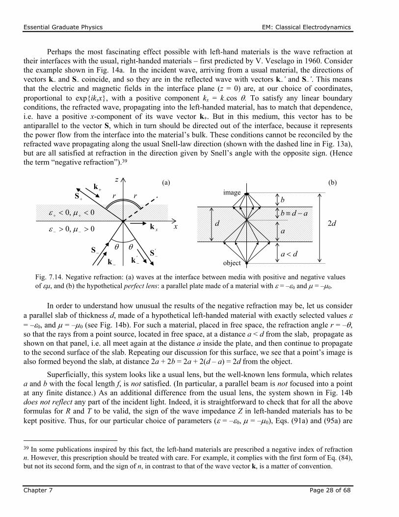
Essential Graduate Physics EM: Classical Electrodynamics
Chapter 7 Page 28 of 68
Perhaps the most fascinating effect possible with left-hand materials is the wave refraction at their interfaces with the usual, right-handed materials – first predicted by V. Veselago in 1960. Consider the example shown in Fig. 14a. In the incident wave, arriving from a usual material, the directions of vectors k– and S– coincide, and so they are in the reflected wave with vectors k–’ and S–’. This means that the electric and magnetic fields in the interface plane (z = 0) are, at our choice of coordinates, proportional to exp{ikxx}, with a positive component kx = k–cos . To satisfy any linear boundary conditions, the refracted wave, propagating into the left-handed material, has to match that dependence, i.e. have a positive x-component of its wave vector k+. But in this medium, this vector has to be antiparallel to the vector S, which in turn should be directed out of the interface, because it represents the power flow from the interface into the material’s bulk. These conditions cannot be reconciled by the refracted wave propagating along the usual Snell-law direction (shown with the dashed line in Fig. 13a), but are all satisfied at refraction in the direction given by Snell’s angle with the opposite sign. (Hence the term “negative refraction”).39
In order to understand how unusual the results of the negative refraction may be, let us consider a parallel slab of thickness d, made of a hypothetical left-handed material with exactly selected values = –0, and = –0 (see Fig. 14b). For such a material, placed in free space, the refraction angle r = –, so that the rays from a point source, located in free space, at a distance a < d from the slab, propagate as shown on that panel, i.e. all meet again at the distance a inside the plate, and then continue to propagate to the second surface of the slab. Repeating our discussion for this surface, we see that a point’s image is also formed beyond the slab, at distance 2a + 2b = 2a + 2(d – a) = 2d from the object.
Superficially, this system looks like a usual lens, but the well-known lens formula, which relates a and b with the focal length f, is not satisfied. (In particular, a parallel beam is not focused into a point at any finite distance.) As an additional difference from the usual lens, the system shown in Fig. 14b does not reflect any part of the incident light. Indeed, it is straightforward to check that for all the above formulas for R and T to be valid, the sign of the wave impedance Z in left-handed materials has to be kept positive. Thus, for our particular choice of parameters ( = –0, = –0), Eqs. (91a) and (95a) are
39 In some publications inspired by this fact, the left-hand materials are prescribed a negative index of refraction n. However, this prescription should be treated with care. For example, it complies with the first form of Eq. (84), but not its second form, and the sign of n, in contrast to that of the wave vector k, is a matter of convention.
Fig. 7.14. Negative refraction: (a) waves at the interface between media with positive and negative values of , and (b) the hypothetical perfect lens: a parallel plate made of a material with = –0 and = –0.
z
r
0,0
0,0
k
S
S'k
'S
r
xk
k
x
(a) (b)
da
a
adb
b
d d2
object
image

Essential Graduate Physics EM: Classical Electrodynamics
Chapter 7 Page 29 of 68
valid with Z+ = Z- = Z0 and cos r = cos = 1, giving R = 0 for any linear polarization, and hence for any other wave polarization – circular, elliptic, natural, etc.
The perfect lens suggestion has triggered a wave of efforts to implement left-hand materials experimentally. (Attempts to find such materials in nature have failed so far.) Most progress in this direction has been achieved using the so-called metamaterials, which are essentially quasi-periodic arrays of specially designed electromagnetic resonators, ideally with high density n >> -3. For example, Fig. 15 shows the metamaterial that was used for the first demonstration of negative refractivity in the microwave region – for ~10-GHz frequencies.40 It combines straight strips of a metallic film, working as lumped resonators with a large electric dipole moment (hence strongly coupled to the wave’s electric field E), and several almost-closed film loops (so-called split rings), working as lumped resonators with large magnetic dipole moments, coupled to the field H. The negative refractivity is achieved by designing the resonance frequencies close to each other. More recently, metamaterials with negative refractivity were demonstrated in the optical range,41 although to the best of my knowledge, their relatively large absorption still prevents practical applications.
This progress has stimulated the development of other potential uses of metamaterials (not necessarily the left-handed ones), in particular, designs of nonuniform systems with engineered distributions (r, ) and (r, ) that may provide electromagnetic wave propagation along the desired paths, e.g., around a certain region of space, making it virtually invisible for an external observer – so far, within a limited frequency range.42
As was mentioned in Sec. 5.5, another way to reach negative values of () is to place a ferromagnetic material into such an external dc magnetic field that the frequency r of the ferromagnetic resonance is somewhat lower than . If thin layers of such a material (e.g., nickel) are interleaved with layers of a non-magnetic very good conductor (such as copper), the resulting metamaterial has an average value of () – say, positive, but substantially below 0. According to Eq. (6.33), the skin-depth s of such a material may be larger than that of the good conductor alone, enforcing a more uniform distribution of the ac current flowing along the layers, and hence making the energy losses lower than in the good conductor alone. This effect may be useful, in particular, for electronic circuit interconnects.43
40 R. Shelby et al., Science 292, 77 (2001); J. Wilson and Z. Schwartz, Appl. Phys. Lett. 86, 021113 (2005). 41 See, e.g., J. Valentine et al., Nature 455, 376 (2008). 42 For a review of such “invisibility cloaks”, see, e.g., B. Wood, Comptes Rendus Physique 10, 379 (2009). 43 See, for example, N. Sato et al., J. Appl. Phys. 111, 07A501 (2012), and references therein.
Fig. 7.15. An artificial left-hand material providing negative refraction at microwave frequencies ~10 GHz. The original by Jeffrey D. Wilson (in the public domain) is available at https://en.wikipedia.org/wiki/Metamaterial.

Essential Graduate Physics EM: Classical Electrodynamics
Chapter 7 Page 30 of 68
7.5. Transmission lines: TEM waves
So far, we have analyzed plane electromagnetic waves, implying that their cross-section is infinite – evidently, the unrealistic assumption. The cross-section may be limited, still sustaining wave propagation along wave transmission lines:44 long, uniform structures made of either good conductors or dielectrics. Let us first discuss the first option, using the following simplifying assumptions:
(i) the structure is a cylinder (not necessarily with a round cross-section, see Fig. 16) filled with a usual (right-handed), uniform dielectric material with negligible energy losses (” = ” = 0), and
(ii) the wave attenuation due to the skin effect is also negligibly low. (As Eq. (78) indicates, for that the characteristic size a of the line’s cross-section has to be much larger than the skin-depth s of its wall material. The energy dissipation effects will be analyzed in Sec. 9 below.)
With such exclusion of energy losses, we may look for a particular solution of the macroscopic Maxwell equations in the form of a monochromatic wave traveling along the line:
)()( ),(Re),(,),(Re),( tzzkitzzki eyxteyxt
HrHErE , (7.98)
with real kz, where the z-axis is directed along the transmission line – see Fig. 16. Note that this form allows an account for a substantial coordinate dependence of the electric and magnetic field within the plane [x, y] of the transmission line’s cross-section, as well as for longitudinal components of the fields, so that the solution (98) is substantially more complex than the plane waves we have discussed above. We will see in a minute that as a result of this dependence, the parameter kz may be very much different from its plane-wave value (13), k ()1/2, in the same material, at the same frequency.
In order to describe these effects quantitatively, let us decompose the complex amplitudes of the wave’s fields into their longitudinal and transverse components (Fig. 16):45
tzztzz HE HnHEnE , . (7.99)
44 Another popular term is the waveguide, but it is typically reserved for the transmission lines with singly-connected cross-sections, to be analyzed in the next section. The first structure for guiding waves was proposed by J. J. Thomson in 1893, and experimentally tested by O. Lodge in 1894. 45 For the notation simplicity, I am dropping index in the complex amplitudes of the field components, and also have dropped the argument in kz and Z, even though these parameters may depend on the wave’s frequency rather substantially – see below.
Fig. 7.16. Electric field’s decomposition in a transmission line (in particular, a waveguide). 0
z
x
y
tE
zzE n E

Essential Graduate Physics EM: Classical Electrodynamics
Chapter 7 Page 31 of 68
Plugging Eqs. (98)-(99) into the source-free Maxwell equations (2), and requiring the longitudinal and transverse components to be balanced separately, we get
,
,
,
zztt
zztt
zztttzz
Eik
Hi
Eiik
E
nE
nHEn
.
,
,
zztt
zztt
zztttzz
Hik
Ei
Hiik
H
nH
nEHn
(7.100)
where t is the 2D del operator acting in the transverse plane [x, y] only, i.e. the usual , but with /z = 0. The system of Eqs. (100) looks even bulkier than the original equations (2), but it is much simpler for analysis. Indeed, eliminating the transverse components from these equations (or, even simpler, just plugging Eq. (99) into Eqs. (3) and keeping only their z-components), we get a pair of self-consistent equations for the longitudinal components of the fields, 46
0,0 2222 zttztt HkEk , (7.101)
where k is still defined by Eq. (13), k = ()1/2, while
22222zzt kkkk (7.102)
After the distributions Ez(x,y) and Hz(x,y) have been found from these equations, they provide right-hand sides for the rather simple, closed system of equations (100) for the transverse components of field vectors. Moreover, as we will see below, each of the following three types of solutions:
(i) with Ez = 0 and Hz = 0 (called the transverse electromagnetic, or TEM waves),
(ii) with Ez = 0, but Hz 0 (called either the TE waves or, more frequently, H-modes), and
(iii) with Ez 0, but Hz = 0 (the so-called TM waves or E-modes),
has its own dispersion law and hence its own wave propagation velocity; as a result, these modes (i.e. the field distribution patterns) may be considered separately.
In the balance of this section, we will focus on the simplest, TEM waves (i), with no longitudinal components of either field. For them, the top two equations of the system (100) immediately give Eqs. (6) and (13), and kz = k. In plain English, this means that E = Et and H = Ht are proportional to each other and are mutually perpendicular (just as in the plane wave) at each point of the cross-section, and that the TEM wave’s impedance Z E/H and dispersion law (k), and hence the propagation speed, are the same as in a plane wave in the same material. In particular, if and are frequency-independent within a certain frequency range, the dispersion law within this range is linear, = k/()1/2, and the wave’s speed does not depend on its frequency. For practical applications to telecommunications, this is a very important advantage of the TEM waves over their TM and TE counterparts – to be discussed below.
Unfortunately for practice, such waves cannot propagate in every transmission line. To show this, let us have a look at the two last lines of Eqs. (100). For the TEM waves (Ez = 0, Hz = 0, kz = k), they are reduced to merely
46 The wave equation represented in the form (101), even with the 3D Laplace operator, is called the Helmholtz equation, named after Hermann von Helmholtz (1821-1894) – the mentor of H. Hertz and M. Planck, among many others.
2D Helmholtz equations for
Ez and Hz
Wave vector component
balance

Essential Graduate Physics EM: Classical Electrodynamics
Chapter 7 Page 32 of 68
.0,0
,0,0
tttt
tttt
HE
HE
(7.103)
Within the coarse-grain description of the conducting walls of the line (i. e., neglecting the skin depth in comparison with the cross-section dimensions), we have to require that inside them, E = H = 0. Close to a wall but outside it, the normal component En of the electric field may be different from zero, because surface charges may sustain its jump – see Sec. 2.1, in particular Eq. (2.3). Similarly, the tangential component H of the magnetic field may have a finite jump at the surface due to skin currents – see Sec. 6.3, in particular Eq. (6.38). However, the tangential component of the electric field and the normal component of the magnetic field cannot experience such jumps, and in order to have them equal to zero inside the walls they have to equal zero just outside the walls as well:
0,0 nHE . (7.104)
But the left columns of Eqs. (103) and (104) coincide with the formulation of the 2D boundary problem of electrostatics for the electric field induced by electric charges of the conducting walls, with the only difference that in our current case the value of actually means (). Similarly, the right columns of those relations coincide with the formulation of the 2D boundary problem of magnetostatics for the magnetic field induced by currents in the walls, with (). The only difference is that in our current, coarse-grain approximation the magnetic fields cannot penetrate into the conductors.
Now we immediately see that in waveguides with a singly-connected wall, for example, a hollow conducting tube (see, e.g., Fig. 16), the TEM waves are impossible, because there is no way to create a non-zero electrostatic field inside a conductor with such cross-section. However, such fields (and hence the TEM waves) are possible in structures with cross-sections consisting of two or more disconnected (galvanically-insulated) parts – see, e.g., Fig. 17.
In order to derive “global” relations for such a transmission line, let us consider the contour C drawn very close to the surface of one of its conductors – see, e.g., the red dashed line in Fig. 17. We can consider it, on one hand, as the cross-section of a cylindrical Gaussian volume of a certain elementary length dz << 2/k. Using the generalized Gauss law (3.34), we get
Cnt drE , (7.105)
where (not to be confused with the wavelength !) is the complex amplitude of the linear density of the electric charge of the conductor. On the other hand, the same contour C may be used in the generalized Ampère law (5.116) to write
Fig. 7.17. An example of the cross-section of a transmission line that may support the TEM wave propagation.
tE
tH C

Essential Graduate Physics EM: Classical Electrodynamics
Chapter 7 Page 33 of 68
IdrC
t H , (7.106)
where I is the total current flowing along the conductor (or rather its complex amplitude). But, as was mentioned above, in the TEM wave the ratio Et/Ht of the field components participating in these two integrals is constant and equal to Z = (/)1/2, so that Eqs. (105)-(106) give the following simple relation between the “global” variables of the conductor:
kZI
2/1
/. (7.107)
This important relation may be also obtained in a different way; let me describe it as well, because (as we will see below) it has an independent heuristic value. Let us consider a small segment dz << = 2/k of the line’s conductor, and apply the electric charge conservation law (4.1) to the instant values of the linear charge density and current. The cancellation of dz in both parts yields
z
tzI
t
tz
),(),(. (7.108)
If we accept the sinusoidal waveform, exp{i(kz – t)}, for both these variables, we immediately recover Eq. (107) for their complex amplitudes, showing that this relation expresses just the charge continuity law.
The global equation (108) may be made more specific in the case when the frequency dependence of and is negligible, and the transmission line consists of just two isolated conductors – see, e.g., Fig. 17. In this case, to have the wave localized in the space near the two conductors, we need a sufficiently fast decrease of its electric field at large distances. For that, their linear charge densities for each value of z should be equal and opposite, and we can simply relate them to the potential difference V between the conductors:
,),(
),(0C
tzV
tz
(7.109)
where C0 is the mutual capacitance of the conductors (per unit length) – which was repeatedly discussed in Chapter 2. Then Eq. (108) takes the following form:
z
tzI
t
tzVC
),(),(0 . (7.110)
Next, let us consider the contour shown with the red dashed line in Fig. 18 (which shows a cross-section of the transmission line by a plane containing the wave propagation axis z), and apply to it the Faraday induction law (6.3).
Fig. 7.18. Electric current, magnetic flux, and voltage in a two-conductor transmission line.
),( tzI dzz
ItzI
),(
dz
dztzILd ),(0),( tzV dzz
VtzV
),(

Essential Graduate Physics EM: Classical Electrodynamics
Chapter 7 Page 34 of 68
Since, in the coarse-grain approximation, the electric field inside the conductors (in Fig. 18, on the horizontal segments of the contour) vanishes, the total e.m.f. equals the difference of the voltages V at the ends of the segment dz, while the only source of the magnetic flux through the area limited by the contour is the (equal and opposite) currents I in the conductors, we can use Eq. (5.70) to express it. As a result, canceling dz in both parts of the equation, we get
z
tzV
t
tzIL
),(),(0 , (7.111)
where L0 is the mutual inductance of the conductors per unit length. The only difference between this L0 and the dc mutual inductances discussed in Chapter 5 is that at the high frequencies we are analyzing now, L0 should be calculated neglecting the magnetic field penetration into the conductors. (In the dc case, we had the same situation for superconductor electrodes, within their coarse-grain, ideal-diamagnetic description.)
The system of Eqs. (110) and (111) is frequently called the telegrapher’s equations. Combined, they give for any “global” variable f (either V, or I, or ) the usual 1D wave equation,
02
2
002
2
t
fCL
z
f, (7.112)
which describes dispersion-free TEM wave’s propagation. Again, this equation is only valid within the frequency range where the frequency dependence of both and is negligible. If it is not so, the global approach may still be used for sinusoidal waves f = Re[fexp{i(kz – t)}]. Repeating the above arguments, instead of Eqs. (110)-(111) we get a more general system of two algebraic equations
,, 00 kVILkIVC (7.113)
in which L0 and C0 may now depend on frequency. These equations are consistent only if
22
2
00
1
v
kCL . (7.114)
Besides the fact we have already known (that the TEM wave’s speed is the same as that of the plane wave), Eq. (114) gives us the result that I confess was not emphasized enough in Chapter 5: the product L0C0 does not depend on the shape or size of line’s cross-section provided that the magnetic field’s penetration into the conductors is negligible). Hence, if we have calculated the mutual capacitance C0 of a system of two cylindrical conductors, the result immediately gives us their mutual inductance: L0 = /C0. This relationship stems from the fact that both the electric and magnetic fields may be expressed via the solution of the same 2D Laplace equation for the system’s cross-section.
With Eq. (114) satisfied, any of Eqs. (113) gives the same result for the following ratio:
2/1
0
0
C
L
I
VZW
, (7.115)
which is called the transmission line’s impedance. This parameter has the same dimensionality (in SI units, ohms) as the wave impedance (7),
L0C0 product invariance
Transmission line’s TEM Impedance

Essential Graduate Physics EM: Classical Electrodynamics
Chapter 7 Page 35 of 68
2/1
H
EZ , (7.116)
but these parameters should not be confused, because ZW depends on cross-section’s geometry, while Z does not. In particular, ZW is the only important parameter of a transmission line for its matching with a lumped load circuit (Fig. 19) in the important case when both the cable cross-section’s size and the load’s linear dimensions are much smaller than the wavelength.47
Indeed, in this case, we may consider the load in the quasistatic limit and write
)()()( 00 zIZzV L , (7.117)
where ZL() is the (generally complex) impedance of the load. Taking V(z,t) and I(z,t) in the form similar to Eqs. (61) and (62), and writing the two Kirchhoff’ s circuit laws for the point z = z0, we get for the reflection coefficient a result similar to Eq. (68):
.)(
)(
WL
WL
ZZ
ZZR
(7.118)
This formula shows that for the perfect matching (i.e. the total wave absorption in the load), the load’s impedance ZL() should be real and equal to ZW – but not necessarily to Z.
As an example, let us consider one of the simplest (and most practically important) transmission lines: the coaxial cable (Fig. 20).48
For this geometry, we already know the expressions for both C0 and L0,49 though they have to be modified for the dielectric and magnetic constants, and the magnetic field’s non-penetration into the conductors. As a result of such (elementary) modification, we get the formulas,
47 The ability of TEM lines to have such a small cross-section is their another important practical advantage. 48 It was invented by the same O. Heaviside in 1880. 49 See, respectively, Eqs. (2.49) and (5.79).
ab
a0
,
Fig. 7. 20. The cross-section of a coaxial cable with (possibly, dispersive) dielectric filling.
)(LZWZV Fig. 7.19. Passive, lumped
termination of a TEM transmission line.
z0z
I
Essential Graduate Physics EM: Classical Electrodynamics
Chapter 7 Page 36 of 68
)/ln(2
,)/ln(
200 abL
abC
, (7.119)
illustrating that the universal relationship (114) is indeed valid. For the cable’s impedance (115), Eqs. (119) yield a geometry-dependent value
Zab
Zab
ZW
2
)/ln(
2
)/ln(2/1
. (7.120)
For the standard TV antenna cables (such as RG-6/U, with b/a ~ 3, /0 2.2), ZW = 75 ohms, while for most computer component connections, coaxial cables with ZW = 50 ohms (such as RG-58/U) are prescribed by electronic engineering standards. Such cables are broadly used for the transmission of electromagnetic waves with frequencies up to 1 GHz over distances of a few km, and up to ~20 GHz on the tabletop scale (a few meters), limited by wave attenuation – see Sec. 9 below.
Moreover, the following two facts enable a wide application, in electrical engineering and physical experiment, the coaxial-cable-like systems. First, as Eq. (5.78) shows, in a cable with a << b, most wave’s energy is localized near the internal conductor. Second, the theory to be discussed in the next section shows that excitation of other (H- and E-) waves in the cable are impossible until the wavelength becomes smaller than ~(a + b). As a result, the TEM mode propagation in a cable with a << b < / is not much affected even if the internal conductor is not straight, but is bent – for example, into a helix – see, e.g., Fig. 21.
In such a system, called the traveling-wave tube, a quasi-TEM wave propagates, with velocity v = 1/()1/2 ~ c, along the helix’ length, so that the velocity’s component along the cable’s axis may be made close to the velocity u << c of the electron beam moving ballistically along the tube’s axis, enabling their effective interaction, and as a result, a length-accumulating amplification of the wave.50
Another important example of a TEM transmission line is a set of two parallel wires. In the form of twisted pairs,51 they allow communications, in particular long-range telephone and DSL Internet connections, at frequencies up to a few hundred kHz, as well as relatively short, multi-line Ethernet and
50 Very unfortunately, in this course I will not have time/space to discuss even the (rather elegant) basic theory of such devices. The reader interested in this field may be referred, for example, to the detailed monograph by J. Whitaker, Power Vacuum Tubes Handbook, 3rd ed., CRC Press, 2017. 51 Such twisting, around the line’s axis, reduces the crosstalk between adjacent lines, and the parasitic radiation at their bends.
Coaxial cable’s C0 and L0
Fig. 7.21. A typical traveling-wave tube: (1) electron gun, (2) ac input, (3) beam-focusing magnets, (4) wave attenuator, (5) helix coil, (6) ac output, (7) vacuum tube, (8) electron collector. Adapted from https://en.wikipedia.org/wiki/Traveling-wave_tube under the Creative Commons BY-SA 3.0 license.

Essential Graduate Physics EM: Classical Electrodynamics
Chapter 7 Page 37 of 68
TV cables at frequencies up to ~ 1 GHz, limited mostly by the mutual interference (“crosstalk”) between the individual lines of the same cable, and the unintentional radiation of the wave into the environment.
7.6. Waveguides: H and E waves
Let us now return to Eqs. (100) and explore the H- and E-waves – with, respectively, either Hz or Ez different from zero. At the first sight, they may seem more complex. However, Eqs. (101), which determine the distribution of these longitudinal components over the cross-section, are just the 2D Helmholtz equations for scalar functions. For simple cross-section geometries, they may be readily solved using the methods discussed for the Laplace equation in Chapter 2, in particular the variable separation. After the solution of such an equation has been found, the transverse components of the fields may be calculated by differentiation, using the simple formulas,
,)(,)(22
ztzztz
ttztzztz
tt E
Z
kHk
k
iHkZEk
k
i nHnE (7.121)
which follow from the two equations in the first line of Eqs. (100).52
In comparison with the boundary problems of electro- and magnetostatics, the only conceptually new feature of Eqs. (101) is that they form the so-called eigenproblems, with typically many solutions (eigenfunctions), each describing a specific wave mode, and corresponding to a specific eigenvalue of the parameter kt. The good news here is that these values of kt are determined by this 2D boundary problem and hence do not depend on kz. As a result, the dispersion law (kz) of any mode, which follows from the last form of Eq. (102),
2/12c
22
2/122
z
tz kvkk
, (7.122)
is functionally similar for all modes. It is also similar to that of plane waves in plasma (see Eq. (38), Fig. 6, and their discussion in Sec. 2), with the only differences that the speed in light c is generally replaced with v = 1/()1/2, i.e. the speed of the plane (or any TEM) waves in the medium filling the waveguide, and that p is replaced with the so-called cutoff frequency
,c tvk (7.123)
specific for each mode. (As Eq. (101) implies, and as we will see from several examples below, kt has the order of 1/a, where a is the characteristic dimension of waveguide’s cross-section, so that the critical value of the free-space wavelength 2c/ is of the order of a.) Below the cutoff frequency of each particular mode, such wave cannot propagate in the waveguide.53 As a result, the modes with the lowest
52 For the derivation of Eqs. (121), one of two linear equations (100) should be first vector-multiplied by nz. Note that this approach could not be used to analyze the TEM waves, because for them kt = 0, Ez = 0, Hz = 0, and Eqs. (121) yield uncertainty. 53 An interesting recent twist in the ideas of electromagnetic metamaterials (mentioned in Sec. 5 above) is the so-called -near-zero materials, designed to have the effective product much lower than 00 within certain frequency ranges. Since at these frequencies the speed v (4) becomes much lower than c, the cutoff frequency (123) virtually vanishes. As a result, the waves may “tunnel” through very narrow sections of metallic
Universal dispersion
relation

Essential Graduate Physics EM: Classical Electrodynamics
Chapter 7 Page 38 of 68
values of c present special practical interest, because the choice of the signal frequency between the two lowest values of the cutoff frequency (123) guarantees that the waves propagate in the form of only one mode, with the lowest kt. Such a choice enables engineers to simplify the excitation of the desired mode by wave generators, and to avoid the parasitic transfer of electromagnetic wave energy to undesirable modes by (virtually unavoidable) small inhomogeneities of the system.
The boundary conditions for the Helmholtz equations (101) depend on the propagating wave type. For the E-modes, with Hz = 0 but Ez 0, the condition E = 0 immediately gives
,0CzE (7.124)
where C is the inner contour limiting the conducting wall’s cross-section. For the H-modes, with Ez = 0 but Hz 0, the boundary condition is slightly less obvious and may be obtained using, for example, the second equation of the system (100), vector-multiplied by nz. Indeed, for the component normal to the conductor surface, the result of such multiplication is
n
H
Z
kiik z
ntzntz
EnH )( . (7.125)
But the first term on the left-hand side of this relation must be zero on the wall surface, because of the second of Eqs. (104), while according to the first of Eqs. (104), the vector Et in the second term cannot have a component tangential to the wall. As a result, the vector product in that term cannot have a normal component, so that the term should equal zero as well, and Eq. (125) is reduced to
0
Cz
n
H. (7.126)
Let us see how does all this machinery work for a simple but practically important case of a metallic-wall waveguide with a rectangular cross-section – see Fig. 22
In the natural Cartesian coordinates, shown in this figure, both Eqs. (101) take the simple form
modes.-for ,
modes,-for , where,02
2
2
2
2
HH
EEffk
yx z
zt (7.127)
From Chapter 2 we know that the most effective way of solution of such equations in a rectangular region is the variable separation, in which the general solution is represented as a sum of partial solutions of the type
waveguides filled with such materials – see, e.g., M. Silveirinha and N. Engheta, Phys. Rev. Lett. 97, 157403 (2006).
a
b
0 x
y
Fig. 7.22. A rectangular waveguide, and the transverse field distribution in its fundamental mode H10 (schematically).
EtH
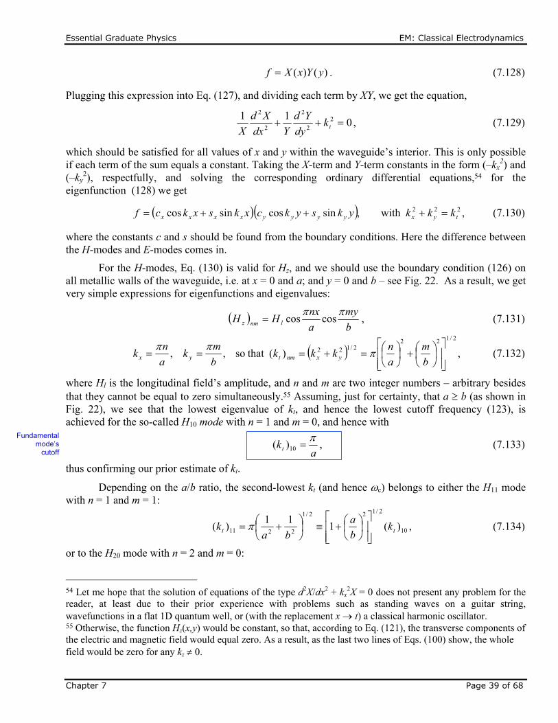
Essential Graduate Physics EM: Classical Electrodynamics
Chapter 7 Page 39 of 68
)()( yYxXf . (7.128)
Plugging this expression into Eq. (127), and dividing each term by XY, we get the equation,
011 2
2
2
2
2
tkdy
Yd
Ydx
Xd
X, (7.129)
which should be satisfied for all values of x and y within the waveguide’s interior. This is only possible if each term of the sum equals a constant. Taking the X-term and Y-term constants in the form (–kx
2) and (–ky
2), respectfully, and solving the corresponding ordinary differential equations,54 for the eigenfunction (128) we get
222with ,sincossincos tyxyyyyxxxx kkkyksykcxksxkcf , (7.130)
where the constants c and s should be found from the boundary conditions. Here the difference between the H-modes and E-modes comes in.
For the H-modes, Eq. (130) is valid for Hz, and we should use the boundary condition (126) on all metallic walls of the waveguide, i.e. at x = 0 and a; and y = 0 and b – see Fig. 22. As a result, we get very simple expressions for eigenfunctions and eigenvalues:
b
my
a
nxHH lnmz
coscos , (7.131)
,)( that so,,
2/1222/122
b
m
a
nkkk
b
mk
a
nk yxnmtyx
(7.132)
where Hl is the longitudinal field’s amplitude, and n and m are two integer numbers – arbitrary besides that they cannot be equal to zero simultaneously.55 Assuming, just for certainty, that a b (as shown in Fig. 22), we see that the lowest eigenvalue of kt, and hence the lowest cutoff frequency (123), is achieved for the so-called H10 mode with n = 1 and m = 0, and hence with
a
kt
10)( , (7.133)
thus confirming our prior estimate of kt.
Depending on the a/b ratio, the second-lowest kt (and hence c) belongs to either the H11 mode with n = 1 and m = 1:
10
2/122/1
2211 )(111
)( tt kb
a
bak
, (7.134)
or to the H20 mode with n = 2 and m = 0:
54 Let me hope that the solution of equations of the type d2X/dx2 + kx2X = 0 does not present any problem for the
reader, at least due to their prior experience with problems such as standing waves on a guitar string, wavefunctions in a flat 1D quantum well, or (with the replacement x t) a classical harmonic oscillator. 55 Otherwise, the function Hz(x,y) would be constant, so that, according to Eq. (121), the transverse components of the electric and magnetic field would equal zero. As a result, as the last two lines of Eqs. (100) show, the whole field would be zero for any kz 0.
Fundamental mode’s
cutoff

Essential Graduate Physics EM: Classical Electrodynamics
Chapter 7 Page 40 of 68
1020 )(22
)( tt ka
k
. (7.135)
These values become equal at a/b = 3 1.7; in practical waveguides, the a/b ratio is not too far from this value. For example, in the standard X-band (~10-GHz) waveguide WR90, a 2.3 cm (fc c/2 6.5 GHz), and b 1.0 cm.
Now let us have a look at the alternative E-modes. For them, we still should use the general solution (130) with f = Ez, but now with the boundary condition (124). This gives us the eigenfunctions
b
my
a
nxEE lnmz
sinsin , (7.136)
and the same eigenvalue spectrum (132) as for the H modes. However, now neither n nor m can be equal to zero; otherwise Eq. (136) would give the trivial solution Ez(x,y) = 0. Hence the lowest cutoff frequency of TM waves is achieved at the so-called E11 mode with n =1, m = 1, and with the eigenvalue given by Eq. (134), always higher than (kt)10.
Thus the fundamental H10 mode is certainly the most important wave in rectangular waveguides; let us have a better look at its field distribution. Plugging the corresponding solution (131) with n = 1 and m = 0 into the general relation (121), we easily get
,0)(,sin)( 1010 ylz
x Ha
xH
akiH
(7.137)
.sin)(,0)( 1010 a
xZH
kaiEE lyx
(7.138)
This field distribution is (schematically) shown in Fig. 22. Neither of the fields depends on the coordinate y – the feature very convenient, in particular, for microwave experiments with small samples. The electric field has only one (in Fig. 22, vertical) component that vanishes at the side walls and reaches its maximum at the waveguide’s center; its field lines are straight, starting and ending on wall surface charges (whose distribution propagates along the waveguide together with the wave). In contrast, the magnetic field has two non-zero components (Hx and Hz), and its field lines are shaped as horizontal loops wrapped around the electric field maxima.
An important question is whether the H10 wave may be usefully characterized by a unique impedance introduced similarly to ZW of the TEM modes – see Eq. (115). The answer is not, because the main value of ZW is a convenient description of the impedance matching of a transmission line with a lumped load – see Fig. 19 and Eq. (118). As was discussed above, such a simple description is possible (i.e., does not depend on the exact geometry of the connection) only if both dimensions of the line’s cross-section are much less than . But for the H10 wave (and more generally, any non-TEM mode) this is impossible – see, e.g., Eq. (129): its lowest frequency corresponds to the TEM wavelength max = 2/(kt)min = 2/(kt)10 = 2a. (The reader is challenged to find a simple interpretation of this equality.)
Now let us consider metallic-wall waveguides with a round cross-section (Fig. 23a). In this single-connected geometry, the TEM waves are impossible again, while for the analysis of H-modes and E-modes, the polar coordinates {, } are most natural. In these coordinates, the 2D Helmholtz equation (101) takes the following form:
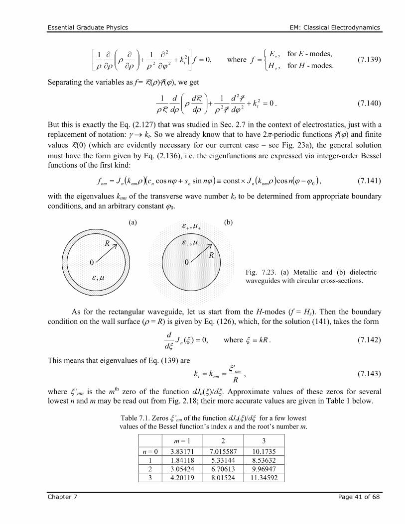
Essential Graduate Physics EM: Classical Electrodynamics
Chapter 7 Page 41 of 68
modes.-for ,
modes,-for , where,0
11 22
2
2 HH
EEffk
z
zt
(7.139)
Separating the variables as f = R()F(), we get
011 2
2
2
2
tk
d
d
d
d
d
d
F
FR
R. (7.140)
But this is exactly the Eq. (2.127) that was studied in Sec. 2.7 in the context of electrostatics, just with a replacement of notation: kt. So we already know that to have 2-periodic functions F() and finite values R(0) (which are evidently necessary for our current case – see Fig. 23a), the general solution must have the form given by Eq. (2.136), i.e. the eigenfunctions are expressed via integer-order Bessel functions of the first kind:
0cosconstsincos nkJnsnckJf nmnnnnmnnm , (7.141)
with the eigenvalues knm of the transverse wave number kt to be determined from appropriate boundary conditions, and an arbitrary constant 0.
As for the rectangular waveguide, let us start from the H-modes (f = Hz). Then the boundary condition on the wall surface ( = R) is given by Eq. (126), which, for the solution (141), takes the form
kRJd
dn
where,0)( . (7.142)
This means that eigenvalues of Eq. (139) are
R
'kk nm
nmt
, (7.143)
where ’nm is the mth zero of the function dJn()/d. Approximate values of these zeros for several lowest n and m may be read out from Fig. 2.18; their more accurate values are given in Table 1 below.
Fig. 7.23. (a) Metallic and (b) dielectric waveguides with circular cross-sections.
R
0
,
(a) (b)
R0
,
,
Table 7.1. Zeros ’nm of the function dJn()/d for a few lowest values of the Bessel function’s index n and the root’s number m.
m = 1 2 3
n = 0 3.83171 7.015587 10.1735 1 1.84118 5.33144 8.53632 2 3.05424 6.70613 9.96947 3 4.20119 8.01524 11.34592
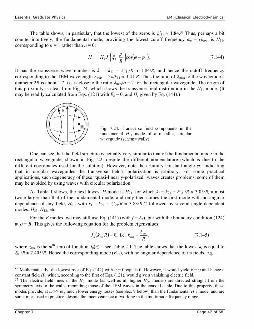
Essential Graduate Physics EM: Classical Electrodynamics
Chapter 7 Page 42 of 68
The table shows, in particular, that the lowest of the zeros is ’11 1.84.56 Thus, perhaps a bit counter-intuitively, the fundamental mode, providing the lowest cutoff frequency c = vknm, is H11, corresponding to n = 1 rather than n = 0:
0111 cos
RJHH '
lz . (7.144)
It has the transverse wave number is kt = k11 = ’11/R 1.84/R, and hence the cutoff frequency corresponding to the TEM wavelength max = 2/k11 3.41 R. Thus the ratio of max to the waveguide’s diameter 2R is about 1.7, i.e. is close to the ratio max/a = 2 for the rectangular waveguide. The origin of this proximity is clear from Fig. 24, which shows the transverse field distribution in the H11 mode. (It may be readily calculated from Eqs. (121) with Ez = 0, and Hz given by Eq. (144).)
One can see that the field structure is actually very similar to that of the fundamental mode in the rectangular waveguide, shown in Fig. 22, despite the different nomenclature (which is due to the different coordinates used for the solution). However, note the arbitrary constant angle 0, indicating that in circular waveguides the transverse field’s polarization is arbitrary. For some practical applications, such degeneracy of these “quasi-linearly-polarized” waves creates problems; some of them may be avoided by using waves with circular polarization.
As Table 1 shows, the next lowest H-mode is H21, for which kt = k21 = ’21/R 3.05/R, almost twice larger than that of the fundamental mode, and only then comes the first mode with no angular dependence of any field, H01, with kt = k01 = ’01/R 3.83/R,57 followed by several angle-dependent modes: H31, H12, etc.
For the E modes, we may still use Eq. (141) (with f = Ez), but with the boundary condition (124) at = R. This gives the following equation for the problem eigenvalues:
,0RkJ nmn i.e. R
k nmnm
, (7.145)
where nm is the mth zero of function Jn() – see Table 2.1. The table shows that the lowest kt is equal to 01/R 2.405/R. Hence the corresponding mode (E01), with no angular dependence of its fields, e.g.
56 Mathematically, the lowest root of Eq. (142) with n = 0 equals 0. However, it would yield k = 0 and hence a constant field Hz, which, according to the first of Eqs. (121), would give a vanishing electric field. 57 The electric field lines in the H01 mode (as well as all higher H0m modes) are directed straight from the symmetry axis to the walls, reminding those of the TEM waves in the coaxial cable. Due to this property, these modes provide, at >> c, much lower energy losses (see Sec. 9 below) than the fundamental H11 mode, and are sometimes used in practice, despite the inconvenience of working in the multimode frequency range.
E
H Fig. 7.24. Transverse field components in the fundamental H11 mode of a metallic, circular waveguide (schematically).

Essential Graduate Physics EM: Classical Electrodynamics
Chapter 7 Page 43 of 68
RJEE lz
010 , (7.146)
has the second-lowest cutoff frequency, ~30% higher than that of the fundamental mode H11.
Finally, let us discuss one more topic of general importance – the number N of electromagnetic modes that may propagate in a waveguide within a certain range of relatively large frequencies >> c. It is easy to calculate for a rectangular waveguide, with its simple expressions (132) for the eigenvalues of {kx, ky}. Indeed, these expressions describe a rectangular mesh on the [kx, ky] plane, so that each point corresponds to the plane area Ak = (/a)(/b), and the number of modes in a large k-plane area Ak >> Ak is N = Ak/Ak = abAk/2 = AAk/2, where A is the waveguide’s cross-section area.58 However, it is frequently more convenient to discuss transverse wave vectors kt of arbitrary direction, i.e. with an arbitrary sign of their components kx and ky. Taking into account that the opposite values of each component actually give the same wave, the actual number of different modes of each type (E- or H-) is a factor of 22 4 lower than was calculated above. This means that the number of modes of both types is
2)2(
2
AAN k . (7.147)
Let me leave it for the reader to find hand-waving (but convincing :-) arguments that this mode counting rule is valid for waveguides with cross-sections of any shape, and any boundary conditions on the walls, provided that N >> 1.
7.7. Dielectric waveguides, optical fibers, and paraxial beams
Now let us discuss electromagnetic wave propagation in dielectric waveguides. The simplest, step-index waveguide (see Figs. 23b and 25) consists of an inner core and an outer shell (in the optical fiber technology lingo, called cladding) with a higher wave propagation speed, i.e. a lower index of refraction:
,, i.e., kknnvv . (7.148)
at the same frequency. (In most cases the difference is achieved due to that in the electric permittivity, + < -, while magnetically both materials are virtually passive: - + 0, so that their refraction indices n, defined by Eq. (84), are very close to (/0)
1/2; I will limit my discussion to this approximation.)
The basic idea of waveguide’s operation may be readily understood in the limit when the wavelength is much smaller than the characteristic size R of the core’s cross-section. In this “geometric optics” limit, at the distances of the order of from the core-to-cladding interface, which determines the wave reflection, we can neglect the interface’s curvature and approximate its geometry with a plane. As we know from Sec. 4, if the angle of the wave’s incidence on such an interface is larger than the critical value c specified by Eq. (85), the wave is totally reflected. As a result, the waves launched into the fiber core at such “grazing” angles, propagate inside the core, being repeatedly reflected from the cladding – see Fig. 25.
58 This formula ignores the fact that, according to the above analysis, some modes (with n = 0 and m = 0 for the H modes, and n = 0 or m = 0 for the E modes) are forbidden. However, for N >> 1, the associated corrections of Eq. (147) are negligible.
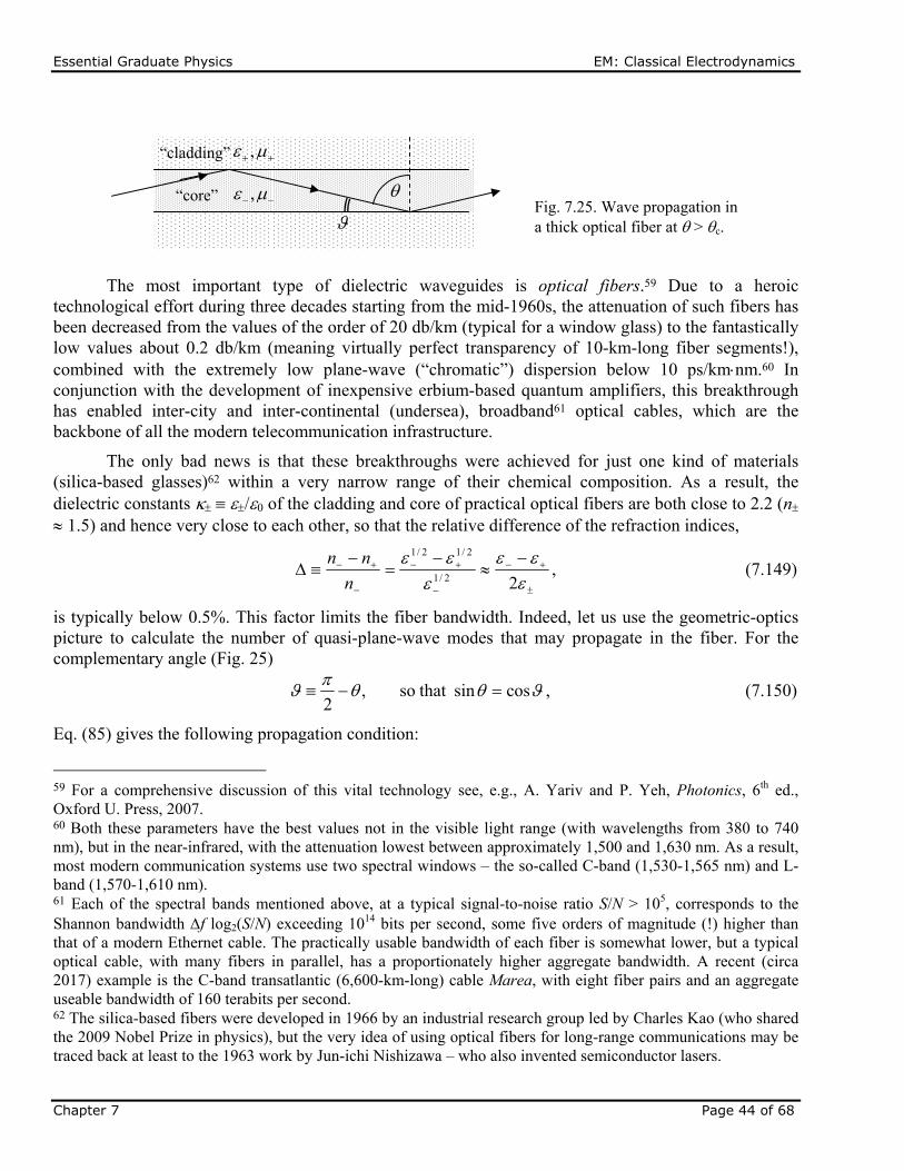
Essential Graduate Physics EM: Classical Electrodynamics
Chapter 7 Page 44 of 68
The most important type of dielectric waveguides is optical fibers.59 Due to a heroic technological effort during three decades starting from the mid-1960s, the attenuation of such fibers has been decreased from the values of the order of 20 db/km (typical for a window glass) to the fantastically low values about 0.2 db/km (meaning virtually perfect transparency of 10-km-long fiber segments!), combined with the extremely low plane-wave (“chromatic”) dispersion below 10 ps/kmnm.60 In conjunction with the development of inexpensive erbium-based quantum amplifiers, this breakthrough has enabled inter-city and inter-continental (undersea), broadband61 optical cables, which are the backbone of all the modern telecommunication infrastructure.
The only bad news is that these breakthroughs were achieved for just one kind of materials (silica-based glasses)62 within a very narrow range of their chemical composition. As a result, the dielectric constants /0 of the cladding and core of practical optical fibers are both close to 2.2 (n 1.5) and hence very close to each other, so that the relative difference of the refraction indices,
,22/1
2/12/1
n
nn (7.149)
is typically below 0.5%. This factor limits the fiber bandwidth. Indeed, let us use the geometric-optics picture to calculate the number of quasi-plane-wave modes that may propagate in the fiber. For the complementary angle (Fig. 25)
cossin that so,2
, (7.150)
Eq. (85) gives the following propagation condition:
59 For a comprehensive discussion of this vital technology see, e.g., A. Yariv and P. Yeh, Photonics, 6th ed., Oxford U. Press, 2007. 60 Both these parameters have the best values not in the visible light range (with wavelengths from 380 to 740 nm), but in the near-infrared, with the attenuation lowest between approximately 1,500 and 1,630 nm. As a result, most modern communication systems use two spectral windows – the so-called C-band (1,530-1,565 nm) and L-band (1,570-1,610 nm). 61 Each of the spectral bands mentioned above, at a typical signal-to-noise ratio S/N > 105, corresponds to the Shannon bandwidth f log2(S/N) exceeding 1014 bits per second, some five orders of magnitude (!) higher than that of a modern Ethernet cable. The practically usable bandwidth of each fiber is somewhat lower, but a typical optical cable, with many fibers in parallel, has a proportionately higher aggregate bandwidth. A recent (circa 2017) example is the C-band transatlantic (6,600-km-long) cable Marea, with eight fiber pairs and an aggregate useable bandwidth of 160 terabits per second. 62 The silica-based fibers were developed in 1966 by an industrial research group led by Charles Kao (who shared the 2009 Nobel Prize in physics), but the very idea of using optical fibers for long-range communications may be traced back at least to the 1963 work by Jun-ichi Nishizawa – who also invented semiconductor lasers.
Fig. 7.25. Wave propagation in a thick optical fiber at > c.
“core”
“cladding”
,
,

Essential Graduate Physics EM: Classical Electrodynamics
Chapter 7 Page 45 of 68
1cosn
n . (7.151)
In the limit << 1, when the incidence angles > c of all propagating waves are very close to /2, and hence the complementary angles are small, we can keep only two first terms in the Taylor expansion of the left-hand side of Eq. (151) and get 22
max . (7.152)
(Even for the higher-end value = 0.005, this critical angle is only ~0.1 radian, i.e. close to 5.) Due to this smallness, we may approximate the maximum transverse component of the wave vector as
kkkkt 2)(sin)( maxmaxmax , (7.153)
and use Eq. (147) to calculate the number N of propagating modes:
2
2
2max
22
22 kR
kRN
. (7.154)
For typical values k = 0.73107 m-1 (corresponding to the free-space wavelength 0 = n = 2n/k 1.3 m), R = 25 m, and = 0.005, this formula gives N 150.
Now we can calculate the geometric dispersion of such a fiber, i.e. the difference of the mode propagation speed, which is commonly characterized in terms of the difference between the wave delay times (traditionally measured in picoseconds per kilometer) of the fastest and slowest modes. Within the geometric optics approximation, the difference of time delays of the fastest mode (with kz = k) and the slowest mode (with kz = k sinc) at distance l is
v
l
n
n
v
l
v
lk
llk
v
lt z
z
z
1sin1 c. (7.155)
For the example considered above, the TEM wave’s speed in the glass, v = c/n 2108 m/s, and the geometric dispersion t/l is close to 25 ps/m, i.e. 25,000 ps/km. (This means, for example, that a 1-ns pulse, being distributed between the modes, would spread to a ~25-ns pulse after passing a just 1-km fiber segment.) This result should be compared with the chromatic dispersion mentioned above, below 10 ps/kmnm, which gives dt/l is of the order of only 1,000 ps/km in the whole communication band d ~ 100 nm. Due to this high geometric dispersion, such relatively thick (2R ~ 50 nm) multi-mode fibers are used for the transfer of signals power over only short distances below ~ 100 m. (As compensation, they may carry relatively large power, beyond 10 mW.)
Long-range telecommunications are based on single-mode fibers, with thin cores (typically with diameters 2R ~ 5 m, i. e. of the order of /1/2). For such structures, Eq. (154) yields N ~ 1, but in this case the geometric optics approximation is not quantitatively valid, and for the fiber analysis, we should get back to the Maxwell equations. In particular, this analysis should take into explicit account the evanescent wave in the cladding, because its penetration depth may be comparable with R.63
63 The following quantitative analysis of the single-mode fibers is very valuable – both for practice and as a very good example of Maxwell equations’ solution. However, its results will not be used in the following parts of the course, so that if the reader is not interested in this topic, they may safely jump to the text following Eq. (181). (I

Essential Graduate Physics EM: Classical Electrodynamics
Chapter 7 Page 46 of 68
Since the cross-section of an optical fiber lacks metallic walls, the Maxwell equations describing them cannot be exactly satisfied with either TEM-wave, or H-mode, or E-mode solutions. Instead, the fibers can carry the so-called HE and EH modes, with both vectors H and E having longitudinal components simultaneously. In such modes, both Ez and Hz inside the core ( R) have a form similar to Eq. (141):
222220 and,0 where,cos kkkknkJff zttnl , (7.156)
where the constant angles 0 may be different for each field. On the other hand, for the evanescent wave in the cladding, we may rewrite Eqs. (101) as
2222222 and,0 where,0 kkkf ztt . (7.157)
Figure 26 illustrates these relations between kt, t, kz, and k; note that the following sum,
2
0222 2)( kk tt , (7.158)
is fixed (at a given frequency) and, for typical fibers, is very small (<< k2). In particular, Fig. 26 shows that neither kt nor t can be larger than [(- – +)0]
1/2 = (2)1/2 k. This means that the depth = 1/t of the wave penetration into the cladding is at least 1/k(2)1/2 = /2(2)1/2 >> /2. This is why the cladding layers in practical optical fibers are made as thick as ~50 m, so that only a negligibly small tail of this evanescent wave field reaches their outer surfaces.
In the polar coordinates, Eq. (157) becomes
011 2
2
2
2
ft
, (7.159)
- the equation to be compared with Eq. (139) for the circular metallic-wall waveguide. From Sec. 2.7 we know that the eigenfunctions of Eq. (159) are the products of the sine and cosine functions of n by a linear combination of the modified Bessel functions In and Kn shown in Fig. 2.22, now of the argument t. The fields have to vanish at , so that only the latter functions (of the second kind) can participate in the solution:
0cos)( nKf tn (7.160)
Now we have to reconcile Eqs. (156) and (160), using the boundary conditions at = R for both longitudinal and transverse components of both fields, with the latter components first calculated using
believe that the discussion of the angular momentum of electromagnetic radiation, starting at that point, is compulsory for every professional physicist.)
2zk 2k2
k 2k
2t
2tk
0222 )( kk
Fig. 7.26. The relation between the transverse exponents kt and t for waves in optical fibers.
Universal relation between kt and t

Essential Graduate Physics EM: Classical Electrodynamics
Chapter 7 Page 47 of 68
Eqs. (121). Such a conceptually simple, but a bit bulky calculation (which I am leaving for the reader’s exercise), yields a system of two linear, homogeneous equations for the complex amplitudes El and Hl, which are compatible if
222
2
2
2
2
222 1111
ttttn
n
tn
n
tn
n
tn
n
t k
k
k
k
R
n
K
'K
J
'J
kK
'Kk
J
'J
k
k
, (7.161)
where the prime signs (as a rare exception in this series) denote the derivatives of each function over its full argument: kt for Jn, and t for Kn.
For any given frequency , the system of equations (158) and (161) determines the values of kt and t, and hence kz. Actually, for any n > 0, this system provides two different solutions: one corresponding to the so-called HE wave, with a larger ratio Ez/Hz, and the EH wave, with a smaller value of that ratio. For angular-symmetric modes with n = 0 (for whom we might naively expect the lowest cutoff frequency), the equations may be satisfied by the fields having just one non-zero longitudinal component (either Ez or Hz), so that the HE modes are the usual E waves, while the EH modes are the H waves. For the H modes, the characteristic equation is reduced to the requirement that the expression in the second parentheses on the left-hand side of Eq. (161) is equal to zero. Using the Bessel function identities J’0 = –J1 and K’0 = –K1, this equation may be rewritten in a simpler form:
)(
)(1
)(
)(1
0
1
0
1
RK
RK
RkJ
RkJ
k t
t
tt
t
t
. (7.162)
Using the universal relation between kt and t given by Eq. (158), we may plot both sides of Eq. (162) as functions of the same argument, say, ktR – see Fig. 27.
The right-hand side of Eq. (162) depends not only on , but also on the dimensionless parameter V defined as the normalized right-hand side of Eq. (158):
2220
22 2)( RkR V . (7.163)
(According to Eq. (154), if V >> 1, it gives twice the number N of the fiber modes – the conclusion confirmed by Fig. 27, taking into account that it describes only the H modes.) Since the ratio K1/K0 is positive for all values of the functions’ argument (see, e.g., the right panel of Fig. 2.22), the right-hand
0 5 103
0
3
Fig. 7.27. Two sides of the characteristic equation (162), plotted as functions of ktR, for two values of its dimensionless parameter: V = 8 (blue line) and V = 3 (red line). Note that according to Eq. (158), the argument of the functions K0 and K1 is tR = [V 2 – (ktR)2]1/2 (V 2 – 2)1/2.
Rkt
RHS
01 11 1202 03LHS

Essential Graduate Physics EM: Classical Electrodynamics
Chapter 7 Page 48 of 68
side of Eq. (162) is always negative, so that the equation may have solutions only in the intervals where the ratio J1/J0 is negative, i.e. at
,..., 12021101 RkRk tt , (7.164)
where nm is the m-th zero of the function Jn() – see Table 2.1. The right-hand side of the characteristic equation (162) diverges at tR 0, i.e. at ktR V, so that no solutions are possible if V is below the critical value Vc = 01 2.405. At this cutoff point, Eq. (163) yields k 01/R(2)1/2. Hence, the cutoff frequency of the lowest H mode corresponds to the TEM wavelength
2/12/1
01max 7.32
2 R
R
. (7.165)
For typical parameters = 0.005 and R = 2.5 m, this result yields max ~ 0.65 m, corresponding to the free-space wavelength 0 ~ 1 m. A similar analysis of the first parentheses on the left-hand side of Eq. (161) shows that at 0, the cutoff frequency for the E modes is similar.
This situation may look exactly like that in metallic-wall waveguides, with no waves possible at frequencies below c, but this is not so. The basic reason for the difference is that in the metallic waveguides, the approach to c results in the divergence of the longitudinal wavelength z 2/kz. On the other hand, in dielectric waveguides, the approach leaves z finite (kz k+). Due to this difference, a certain linear superposition of HE and EH modes with n = 1 can propagate at frequencies well below the cutoff frequency for n = 0, which we have just calculated.64 This mode, in the limit + - (i.e. << 1) allows a very interesting and simple description using the Cartesian (rather than polar) components of the fields, but still expressed as functions of the polar coordinates and . The reason is that this mode is very close to a linearly polarized TEM wave. (Due to this reason, this mode is referred to as LP01.)
Let us select the x-axis parallel to the transverse component of the magnetic field vector at = 0, so that Ex=0 = 0, but Ey=0 0, and Hx=0 0, but Hy=0 = 0. The only suitable solutions of the 2D Helmholtz equation (that should be obeyed not only by the z-components of the field, but also their x- and y-components) are proportional to J0(kt), with zero coefficients for Ex and Hy:
RHkJHHkJEEE ytxtyx for ,0),(),(,0 0000 . (7.166)
Now we can use the last two equations of Eqs. (100) to calculate the longitudinal components of the fields:
cos)(1
,sin)(1
1010 tz
tx
zzt
z
ty
zz kJH
k
ki
x
H
ikHkJE
k
ki
y
E
ikE
, (7.167)
where I have used the following mathematical identities: J’0 = –J1, /x = x/ = cos, and /y = y/ = sin. As a sanity check, we see that the longitudinal component or each field is a (legitimate!) eigenfunction of the type (141), with n = 1. Note also that if kt << kz (this relation is always true if << 1 – see either Eq. (158) or Fig. 26), the longitudinal components of the fields are much smaller than their
64 This fact becomes less surprising if we recall that in the circular metallic waveguide, discussed in Sec. 6, the fundamental mode (H11, see Fig. 23) also corresponded to n = 1 rather than n = 0.
LP01 mode
Essential Graduate Physics EM: Classical Electrodynamics
Chapter 7 Page 49 of 68
transverse counterparts, so that the wave is indeed very close to the TEM one. Because of that, the ratio of the electric and magnetic field amplitudes is also close to that in the TEM wave: E0/H0 Z– Z+.
Now to satisfy the boundary conditions at the core-to-cladding interface ( = R), we need to have a similar angular dependence of these components at R. The longitudinal components of the fields are tangential to the interface and thus should be continuous. Using the solutions similar to Eq. (160) with n = 1, we get
.for ,cos)()(
)(,sin)(
)(
)(10
1
110
1
1 RKHRK
RkJ
k
kiHKE
RK
RkJ
k
kiE t
t
t
z
tzt
t
t
z
tz
(7.168)
For the transverse components, we should require the continuity of the normal magnetic field Hn, for our simple field structure equal to just Hxcos, of the tangential electric field E = Eysin, and of the normal component of Dn = En = Eycos. Assuming that - = + = 0, and + -,
65 we can satisfy these
conditions with the following solutions:
.for ,0),()(
)(),(
)(
)(,0 00
0
000
0
0 RHKHRkK
RkJHKE
RK
RkJEE yt
t
txt
t
tyx
(7.169)
From here, we can calculate components from Ez and Hz, using the same approach as for R:
.for ,cos)()(
)(1
,sin)()(
)(1
100
0
100
0
RKHRK
RkJ
ki
x
H
ikH
KERK
RkJ
ki
y
E
ikE
tt
t
z
tx
zz
tt
t
z
ty
zz
(7.170)
These relations provide the same functional dependence of the fields as Eqs. (167), i.e. the internal and external fields are compatible, but their amplitudes at the interface coincide only if
)(
)(
)(
)(
0
1
0
1
RK
RK
RkJ
RkJk
t
tt
t
tt
. (7.171)
This characteristic equation (which may be also derived from Eq. (161) with n = 1 in the limit 0) looks close to Eq. (162), but functionally is much different from it – see Fig. 28. Indeed, its right-hand side is always positive, and the left-hand side tends to zero at ktR 0. As a result, Eq. (171) may have a solution for arbitrary small values of the parameter V defined by Eq. (163), i.e. for arbitrary low frequencies (large wavelengths). This is why this mode is used in practical single-mode fibers: there are no other modes with wavelength larger than max given by Eq. (165), so that they cannot be unintentionally excited on small inhomogeneities of the fiber.
65 It is the core assumption of this approximate theory, which accounts only for the most important effect of the small difference of dielectric constants + and -: the opposite signs of the differences (k+
2 – kz2) = kt
2 and (k-2 –
kz2) = –t
2. For more discussion of the accuracy of this approximation and some exact results, let me refer the interested reader either to the monograph by A. Snyder and D. Love, Optical Waveguide Theory, Chapman and Hill, 1983, or to Chapter 3 and Appendix B in the monograph by Yariv and Yeh, which was cited above.
LP01 mode: characteristic
equation

Essential Graduate Physics EM: Classical Electrodynamics
Chapter 7 Page 50 of 68
It is easy to use the Bessel function approximations by the first terms of the Taylor expansions (2.132) and (2.157) to show that in the limit V 0, tR tends to zero much faster than ktR V: tR 2exp{-1/ V } << V. This means that the scale c 1/t of the radial distribution of the LP01 wave’s fields in the cladding becomes very large. In this limit, this mode may be interpreted as a virtually TEM wave propagating in the cladding, just slightly deformed (and guided) by the fiber’s core. The drawback of this feature is that it requires very thick cladding, to avoid energy losses in its outer (“buffer” and “jacket”) layers that defend the silica layers from the elements, but lack their low optical absorption. Due to this reason, the core radius is usually selected so that the parameter V is just slightly less than the critical value Vc = 01 2.4 for higher modes, thus ensuring the single-mode operation.
In order to reduce the field spread into the cladding, the step-index fibers discussed above may be replaced with graded-index fibers whose dielectric constant is gradually and slowly decreased from the center to the periphery.66 Keeping only the main two terms in the Taylor expansion of the function () at = 0, we may approximate such reduction as
21)0()( , (7.172)
where –[(d2/d2)/2]=0 is a positive constant characterizing the fiber composition gradient.67 Moreover, if this constant is sufficiently small ( << k2), the field distribution across the fiber’s cross-section may be described by the same 2D Helmholtz equation (101), but with a space-dependent transverse wave vector:68
,022 fktt
where (7.173)
022222222 00 and ,0)0()()( kkkkkk tzt .
66 Due to the difficulty of fabrication of graded-index fibers with wave attenuation below a few dm/km, they are not used as broadly as the step-index ones. 67 For an axially-symmetric smooth function (), the first derivative d/d always vanishes at = 0, so that Eq. (172) does not have a term linear in . 68 This approach is invalid at arbitrary (large) because in the macroscopic Maxwell equations, (r) is under the differentiation sign, and the exact Helmholtz-type equations for fields have additional terms containing .
0 5 1010
0
10
Fig. 7.28. Two sides of the characteristic equation (171) for the LP01 mode, plotted as a function of ktR, for two values of the dimensionless parameter: V = 8 (blue line) and V = 1 (red line).
Rkt
LHSRHS
Essential Graduate Physics EM: Classical Electrodynamics
Chapter 7 Page 51 of 68
Surprisingly for such an axially-symmetric problem, because of its special dependence on the radius, this equation may be most readily solved in the Cartesian coordinates. Indeed, rewriting it as
00)0( 22222
2
2
2
fyxkkyx t , (7.174)
and separating the variables as f = X(x)Y(y), we get
00)0(11 2222
2
2
2
2
yxkkdy
Yd
Ydx
Xd
X t , (7.175)
so that the functions X and Y obey similar differential equations, for example
,00 2222
2
Xxkkdx
Xdx (7.176)
with the separation constants satisfying the following condition:
22222 0)0( ztyx kkkkk . (7.177)
The ordinary differential equation (176) is well known from elementary quantum mechanics, because the stationary Schrödinger equation for one of the most important basic quantum systems, a 1D harmonic oscillator, may be rewritten in this form. Its eigenvalues are very simple:
,...2,1,0,with ,120)(,120)( 2/122/12 mnmkknkk mynx , (7.178)
but the corresponding eigenfunctions Xn(x) and Ym(y) are expressed via not quite elementary functions – the Hermite polynomials.69 For most practical purposes, however, the lowest eigenfunctions X0(x) and Y0(y) are sufficient, because they correspond to the lowest kx,y, and hence the lowest
2/10
20
2min
2 02)()(0 kkkk yxt , (7.179)
and the lowest cutoff frequency. As may be readily verified by substitution to Eq. (176), the eigenfunctions corresponding to this fundamental mode are also simple:
2
0expconst)(
22/1
0
xkxX
, (7.180)
and similarly for Y0(y), so that the field distribution follows the Gaussian function
4/12/1
2
2
0
22/1
00 0/1with ,2
exp)0(2
0exp)0()( ka
af
kff
, (7.181)
where a >> 1/k(0) has the sense of the effective width of the field’s extension in the radial direction, normal to the wave propagation axis z. This is the so-called Gaussian beam, very convenient for some applications.
The Gaussian beam (181) is just one example of the so-called paraxial beams, which may be represented as a result of modulation of a plane wave with a wave number k, by an axially-symmetric
69 See, e.g., QM Sec. 2.9.
Essential Graduate Physics EM: Classical Electrodynamics
Chapter 7 Page 52 of 68
envelope function f(), where {x, y}, with a relatively large effective radius a >> 1/k.70 Such beams give me a convenient opportunity to deliver on the promise made in Sec. 1: calculate the angular momentum L of a circularly polarized wave, propagating in free space, and prove its fundamental relation to the wave’s energy U. Let us start from the calculation of U for a paraxial beam (with an arbitrary, but spatially-localized envelope f) of the circularly polarized waves, with the transverse electric field components given by Eq. (19):
,sin,cos 00 fEEfEE yx (7.182a)
where E0 is the real amplitude of the wave’s electric field at the propagation axis, kz – t + is its total phase, and the two signs correspond to two possible directions of the circular polarization.71 According to Eq. (6), the corresponding transverse components of the magnetic field are
cos,sin0
0
0
0 fZ
EHf
Z
EH yx . (7.182b)
These expressions are sufficient to calculate the energy density (6.113) of the wave,72
22002
0
2200
2200
220
220
2222fE
Z
fEfEHHEEu yxyx
, (7.183)
and hence the full energy (per unit length in the direction z of the wave’s propagation) of the beam:
0
2200
0
2 22 dfEdurudU . (7.184)
However, the transverse fields (182) are insufficient to calculate a non-zero average of L. Indeed, following the angular moment’s definition in mechanics,73 L rp, where p is a particle’s (linear) momentum, we may use Eq. (6.115) for the electromagnetic field momentum’s density g in free space, to define the field’s angular momentum’s density as
HErSrgrl 22
11
cc. (7.185)
Let us use the familiar bac minus cab rule of the vector algebra74 to transform this expression to
ErHHrEErHrnErHHrEl ttzzz HEcc 22
11. (7.186)
70 Note that propagating in a uniform medium, i.e. outside of grade-index fibers or other focusing systems, such beams gradually increase their width a due to diffraction – the effect to be analyzed in the next chapter. 71 For our task of calculation of two quadratic forms of the fields (L and U), their real representation (182) is more convenient than the complex-exponent one. However, for linear manipulations, the latter representation of the circularly-polarized waves, Et = E0f()Re[(nx iny)exp{i}], Ht = (E0/Z0)f()Re[(inx + ny)exp{i}], is usually more convenient, and is broadly used. 72 Note that, in contrast to a linearly-polarized wave (16), the energy density of a circularly-polarized wave does not depend on the full phase – in particular, on t at fixed z, or vice versa. This is natural because its field vectors rotate (keeping their magnitude) rather than oscillate – see Fig. 3b. 73 See, e.g., CM Eq. (1.31). 74 See, e.g., MA Eq. (7.5).
EM field’s angular momentum

Essential Graduate Physics EM: Classical Electrodynamics
Chapter 7 Page 53 of 68
If the field is purely transverse (Ez = Hz = 0), as it is in a strictly plane wave, the first square brackets in the last expression vanish, while the second bracket gives an azimuthal component of l, which oscillates in time, and vanishes at its time averaging. (This is exactly the reason why I have not tried to calculate L at our first discussion of the circularly polarized waves in Sec. 1.)
Fortunately, our discussion of optical fibers, in particular, the derivation of Eqs. (167), (168), and (170), gives us a clear clue on how to resolve this paradox. If the envelope function f() differs from a constant, the transverse wave components (182) alone do not satisfy the Maxwell equations (2b), which necessitate longitudinal components Ez and Hz of the fields, with75
y
H
x
H
z
H
y
E
x
E
z
E yxzyxz
, . (7.187)
However, as these expressions show, if the envelope function f changes very slowly in the sense df/d ~ f/a << kf, the longitudinal components are very small and do not have a back effect on the transverse components. Hence, the above calculation of U is still valid (asymptotically, at ka 0), and we may still use Eqs. (182) on the right-hand side of Eqs. (187),
cossin,sincos0
00 x
f
x
f
Z
E
z
H
x
f
x
fE
z
E zz , (7.188)
and integrate them over z as
.cossin
sincossincos
0
00
x
f
x
f
k
E
dx
fd
x
f
k
Edz
x
f
x
fEEz
(7.189a)
Here the integration constant is taken for zero, because no wave field component may have a time-independent part. Integrating, absolutely similarly, the second of Eqs. (188), we get
.sincos0
0
y
f
x
f
kZ
EH z (7.189b)
With the same approximation, we may calculate the longitudinal (z-) component of l, given by the first term of Eq. (186), keeping only the dominating, transverse fields (182) in the scalar products:
yxzyxztztzz yExEHyHxHEHEl ErHr . (7.190)
Plugging in Eqs. (182) and (189), and taking into account that in free space, k = /c, and hence 1/Z0c2k
= 0/, we get:
d
fdEf
E
y
fy
x
fx
E
y
fy
x
fxf
Elz
22002
200
22200
200
222
ρ . (7.191)
Hence the total angular momentum of the beam (per unit length), is
75 The complex-exponential versions of these equalities are given by the bottom line of Eq. (100).

Essential Graduate Physics EM: Classical Electrodynamics
Chapter 7 Page 54 of 68
0
22200
0
22
200
0
2 2 fdE
dd
fdEdlrdlL zzz . (7.192)
Taking this integral by parts, with the assumption that f 0 at 0 and (at it is true for the Gaussian beam (181) and all realistic paraxial beams), we finally get
0
2200
0
22200 2
df
Edf
ELz . (7.193)
Now comparing this expression with Eq, (184), we see that remarkably, the ratio Lz/U does not depend on the shape and the width of the beam (and of course on the wave’s amplitude E0), so these parameters are very simply and universally related:
U
Lz . (7.194)
Since this relation is valid in the plane-wave limit a , it may be attributed to plane waves as well, with the understanding that in real life they always have some width (“aperture”) restriction.
As the reader certainly knows, in quantum mechanics the energy excitations of any harmonic oscillator of frequency are quantized in the units of , while the internal angular momentum of a particle is quantized in the units of s, where s is its spin. In this context, the classical relation (194) is used in quantum electrodynamics as the basis for treating the electromagnetic field excitation quanta (photons) as some sort of quantum particles with spin s = 1. (Such integer spin also fits the Bose-Einstein statistics of the electromagnetic radiation.)
Unfortunately, I do not have time for a further discussion of the (very interesting) physics of paraxial beams, but cannot help noticing, at least in passing, the very curious effect of helical waves – the beams carrying not only the “spin” momentum (194), but also an additional “orbital” angular momentum. The distribution of their energy in space is not monotonic, as it is in the Gaussian beam (181), but reminds several threads twisted around the propagation axis – hence the term “helical”.76 Mathematically, their field structure is described by the associate Laguerre polynomials – the same special functions that are used for the quantum-mechanical description of hydrogen-like atoms.77 Presently there are efforts to use such beams for the so-called orbital angular momentum (OAM) multiplexing for high-rate information transmission.78
7.8. Resonators
Resonators are distributed oscillators, i.e. structures that may sustain standing waves (in electrodynamics, oscillations of the electromagnetic field) even without an external source, until the oscillation amplitude slowly decreases in time due to unavoidable energy losses. If the resonator quality (described by the so-called Q-factor, which will be defined and discussed in the next section) is high, Q
76 Noticing such solutions of the Maxwell equations may be traced back to at least a 1943 theoretical work by J. Humblet; however, this issue had not been discussed in literature too much until experiments carried out in 1992 – see, e.g. L. Allen et al., Optical Angular Momentum; IOP, 2003. 77 See, e.g., QM Sec. 3.7. 78 See, e.g., J. Wang et al., Nature Photonics 6, 488 (2012).
Angular momentum at circular polarization

Essential Graduate Physics EM: Classical Electrodynamics
Chapter 7 Page 55 of 68
>> 1, this decay takes many oscillation periods. Alternatively, high-Q resonators may sustain high oscillating fields permanently, if driven by relatively weak incident waves.
Conceptually the simplest resonator is the Fabry-Pérot interferometer79 that may be obtained by placing two well-conducting planes parallel to each other.80 Indeed, in Sec. 3 we have seen that if a plane wave is normally incident on such a “perfect mirror”, located at z = 0, its reflection, at negligible skin depth, results in a standing wave described by Eq. (61b):
kzeEtzE iti sin2Re),( 2/
. (7.195)
This wave would not change if we had suddenly put the second mirror (isolating the segment of length l from the external wave source) at any position z = l with sin kl = 0, i.e. with
,....2,1 where, ppkl (7.196)
This condition, which determines the spectrum of eigen- (or own-, or resonance-) frequencies of the resonator of fixed length l,
2/1
1with ,
vpa
vvk pp , (7.197)
has a simple physical sense: the resonator’s length l equals exactly p half-waves of the frequency p. Though this is all very simple, please note a considerable change of philosophy from what we have been doing in the previous sections: the main task of resonator’s analysis is finding its eigenfrequencies p that are now determined by the system geometry rather than by an external wave source.
Before we move to more complex resonators, let us use Eq. (62) to represent the magnetic field in the Fabry-Pérot interferometer:
kzeZ
EtzH ti cos2Re),(
. (7.198)
Expressions (195) and (198) show that in contrast to traveling waves, each field of the standing wave changes simultaneously (proportionately) at all points of the Fabry-Pérot resonator, turning to zero everywhere twice a period. At these instants, the energy of the corresponding field vanishes, but the total energy of oscillations stays constant because the counterpart field oscillates with the phase shift /2. Such behavior is typical for all electromagnetic resonators.
Another, more technical remark is that we can readily get the same results (195)-(198) by solving the Maxwell equations from scratch. For example, we already know that in the absence of dispersion, losses, and sources, they are reduced to the wave equations (3) for any field components. For the Fabry-Pérot resonator’s analysis, we can use the 1D form of these equations, say, for the transverse component of the electric field:
,01
2
2
22
2
Etvz
(7.199)
79 The device is named after its inventors, Charles Fabry and Alfred Pérot; is also called the Fabry-Pérot etalon (meaning “gauge”), because of its initial usage for the light wavelength measurements. 80 The resonators formed by well conducting (usually, metallic) walls are frequently called resonant cavities.

Essential Graduate Physics EM: Classical Electrodynamics
Chapter 7 Page 56 of 68
and solve it as a part of an eigenvalue problem with the corresponding boundary conditions. Indeed, separating time and space variables as E(z, t) = Z(z)T(t), we obtain
0111
2
2
22
2
dt
d
vdz
Zd
Z
TT
. (7.200)
Calling the separation constant k2, we get two similar ordinary differential equations,
,0,0 222
22
2
2
TT
vkdt
dZk
dz
Zd (7.201)
both with sinusoidal solutions, so that the product Z(z)T(t) is a standing wave with the wave vector k and
frequency = kv. (In this form, the equations are valid even in the presence of dispersion, but with a frequency-dependent wave speed: v2 = 1/()().) Now using the boundary conditions E(0, t) = E(l, t) = 0,81 we get the eigenvalue spectrum for kp and hence for p = vkp, given by Eqs. (196) and (197).
Lessons from this simple case study may be readily generalized for an arbitrary resonator: there are (at least :-) two approaches to finding the eigenfrequency spectrum:
(i) We may look at a traveling wave solution and find where reflecting mirrors may be inserted without affecting the wave’s structure. Unfortunately, this method is limited to simple geometries.
(ii) We may solve the general 3D wave equations,
0),(1
2
2
22
tftv
r , (7.202)
for field components, as an eigenvalue problem with appropriate boundary conditions. If the system’s parameters (and hence the coefficient v) do not change in time, the spatial and temporal variables of Eq. (202) may be always separated by taking
)()(),( ttf TR rr , (7.203)
where the function T(t) always obeys the same equation as in Eq. (201), having the sinusoidal solution
of frequency = vk. Plugging this solution back into Eqs. (202), for the spatial distribution of the field, we get the 3D Helmholtz equation,
0)(22 rRk , (7.204)
whose solution (for non-symmetric geometries) may be much more complex.
Let us use these approaches to find the eigenfrequency spectrum of a few simple, but practically important resonators. First of all, the first method is completely sufficient for the analysis of any resonator formed as a fragment of a uniform TEM transmission line (e.g., a coaxial cable), confined with two conducting lids normal to the line’s direction. Indeed, since in such lines kz = k = /v, and the electric field is perpendicular to the propagation axis, e.g., parallel to the lid surface, the boundary conditions are exactly the same as in the Fabry-Pérot resonator, and we again arrive at the eigenfrequency spectrum (197).
81 This is of course the expression of the first of the general boundary conditions (104). The second of these conditions (for the magnetic field) is satisfied automatically for the transverse waves we are considering.
3D Helmholtz equation

Essential Graduate Physics EM: Classical Electrodynamics
Chapter 7 Page 57 of 68
Now let us analyze a slightly more complex system: a rectangular metallic-wall cavity of volume abl – see Fig. 29.
To use the first approach outlined above, let us consider the resonator as a finite-length (z = l) section of the rectangular waveguide stretched along axis z, which was analyzed in detail in Sec. 6. As a reminder, at a < b, in the fundamental H10 traveling wave mode, both vectors E and H do not depend on y, with E having only a y-component. In contrast, H has two components, Hx and Hz, with the phase shift /2 between them, and with Hx having the same phase as Ey – see Eqs. (131), (137), and (138). Hence, if a plane perpendicular to the z-axis, is placed so that the electric field vanishes on it, Hx also vanishes, so that both boundary conditions (104), pertinent to a perfect metallic wall, are fulfilled simultaneously.
As a result, the H10 wave would not be perturbed by two metallic walls separated by an integer number of half-wavelengths z/2 corresponding to the wave number given by the combination of Eqs. (102) and (133):
2
2
2
22/122
avkkk tz
. (7.205)
Using this expression, we see that the smallest of these distances, l = z/2 = /kz, gives the resonance frequency82
2/122
101
lav
, (7.206)
where the indices of show the numbers of half-waves along each dimension of the system, in the order [a, b, l]. This is the lowest (fundamental) eigenfrequency of the resonator (if b < a, l).
The field distribution in this mode is close to that in the corresponding waveguide mode H10 (Fig. 22), with the important difference that the magnetic and electric fields are now shifted by phase /2 both in space and time, just as in the Fabry-Pérot resonator – see Eqs. (195) and (198). Such a time shift allows for a very simple interpretation of the H101 mode, which is especially adequate for very flat resonators, with b << a, l. At the instant when the electric field reaches its maximum (Fig. 30a), i.e. when the magnetic field vanishes in the whole volume, the surface electric charge of the walls (with the areal density = En/) is largest, being localized mostly in the middle of the broadest (in Fig. 30, horizontal) faces of the resonator. At the immediate later times, the walls start to recharge via surface
82 In most electrical engineering handbooks, the index corresponding to the shortest side of the resonator is listed last, so that the fundamental mode is nominated as H110 and its eigenfrequency as 110.
a
b
l
x
y
z
0 Fig. 7.29. Rectangular metallic-wall resonator as a finite section of a waveguide with the cross-section shown in Fig. 22.

Essential Graduate Physics EM: Classical Electrodynamics
Chapter 7 Page 58 of 68
currents, whose density J is largest in the side walls, and reaches its maximal value in a quarter of the oscillation period T = 2/101 – see Fig. 30b.
The currents generate the vortex magnetic field, with looped field lines in the plane of the broadest face of the resonator. The surface currents continue to flow in this direction until (in one more quarter period) the broader walls of the resonator are fully recharged in the polarity opposite to that shown in Fig. 30a. After that, the surface currents start to flow in the direction opposite to that shown in Fig. 30b. This process, which repeats again and again, is conceptually similar to the well-known oscillations in a lumped LC circuit, with the role of (now, distributed) capacitance played mostly by the broadest faces of the resonator, and that of (now, distributed) inductance, by its narrower walls.
In order to generalize the result (206) to higher oscillation modes, the second of the approaches discussed above is more prudent. Separating the variables in the Helmholtz equation (204) as R(r) = X(x)Y(y)Z(z), we see that X, Y, and Z have to be either sinusoidal or cosinusoidal functions of their arguments, with wave vector components satisfying the characteristic equation
2
22222
vkkkk zyx
. (7.207)
In contrast to the wave propagation problem, now we are dealing with standing waves along all three dimensions, and have to satisfy the macroscopic boundary conditions (104) on all sets of parallel walls. It is straightforward to check that these conditions (E = 0, Hn = 0) are fulfilled at the following field component distribution:
,cossinsin
,sincossin
,sinsincos
3
2
1
zkykxkEE
zkykxkEE
zkykxkEE
zyxz
zyxy
zyxx
,sincoscos
,cossincos
,coscossin
3
2
1
zkykxkHH
zkykxkHH
zkykxkHH
zyxz
zyxy
zyxx
(7.208)
with each of the wave vector components having an equidistant spectrum, similar to Eq. (196):
,,,l
pk
b
mk
a
nk zyx
(7.209)
so that the full spectrum of eigenfrequencies is given by the following formula, 2/1222
l
p
b
m
a
nvvknmp
, (7.210)
which is a natural generalization of Eq. (206). Note, however, that of the three integers m, n, and p, at least two have to be different from zero to keep the fields (208) from vanishing at all points.
Fig. 7.30. Fields, charges, and currents in the fundamental (H101)
mode of a rectangular metallic resonator, at two instants separated by t = /2101 – schematically. a
b
0
E
+ ++
-- -
H
JJ
(a) (b)
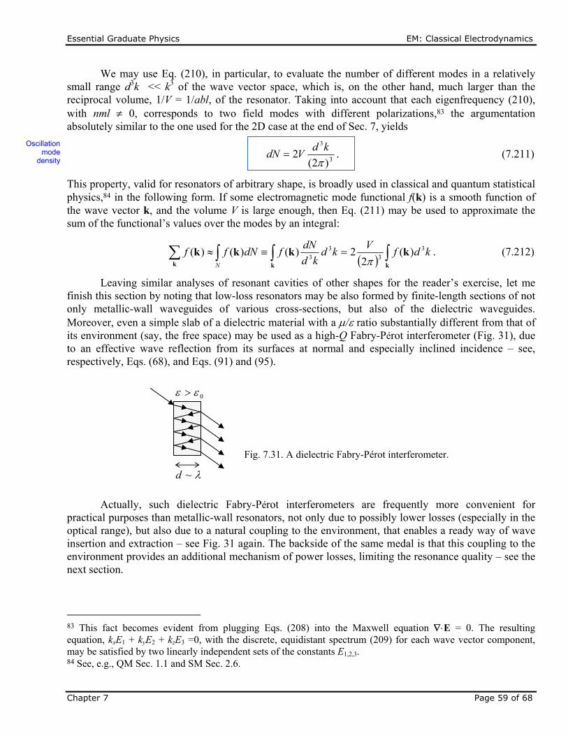
Essential Graduate Physics EM: Classical Electrodynamics
Chapter 7 Page 59 of 68
We may use Eq. (210), in particular, to evaluate the number of different modes in a relatively small range d3k << k3 of the wave vector space, which is, on the other hand, much larger than the reciprocal volume, 1/V = 1/abl, of the resonator. Taking into account that each eigenfrequency (210), with nml 0, corresponds to two field modes with different polarizations,83 the argumentation absolutely similar to the one used for the 2D case at the end of Sec. 7, yields
3
3
)2(2
kd
VdN . (7.211)
This property, valid for resonators of arbitrary shape, is broadly used in classical and quantum statistical physics,84 in the following form. If some electromagnetic mode functional f(k) is a smooth function of the wave vector k, and the volume V is large enough, then Eq. (211) may be used to approximate the sum of the functional’s values over the modes by an integral:
kkk
kkkk kdfV
kdkd
dNfdNff
N
33
33
)(2
2)()()(
. (7.212)
Leaving similar analyses of resonant cavities of other shapes for the reader’s exercise, let me finish this section by noting that low-loss resonators may be also formed by finite-length sections of not only metallic-wall waveguides of various cross-sections, but also of the dielectric waveguides. Moreover, even a simple slab of a dielectric material with a / ratio substantially different from that of its environment (say, the free space) may be used as a high-Q Fabry-Pérot interferometer (Fig. 31), due to an effective wave reflection from its surfaces at normal and especially inclined incidence – see, respectively, Eqs. (68), and Eqs. (91) and (95).
Actually, such dielectric Fabry-Pérot interferometers are frequently more convenient for practical purposes than metallic-wall resonators, not only due to possibly lower losses (especially in the optical range), but also due to a natural coupling to the environment, that enables a ready way of wave insertion and extraction – see Fig. 31 again. The backside of the same medal is that this coupling to the environment provides an additional mechanism of power losses, limiting the resonance quality – see the next section.
83 This fact becomes evident from plugging Eqs. (208) into the Maxwell equation E = 0. The resulting equation, kxE1 + kyE2 + kzE3 =0, with the discrete, equidistant spectrum (209) for each wave vector component, may be satisfied by two linearly independent sets of the constants E1,2,3. 84 See, e.g., QM Sec. 1.1 and SM Sec. 2.6.
Fig. 7.31. A dielectric Fabry-Pérot interferometer.
0
~d
Oscillation mode
density

Essential Graduate Physics EM: Classical Electrodynamics
Chapter 7 Page 60 of 68
7.9. Energy loss effects
The inevitable energy losses (“dissipation”) in passive media lead, in two different situations, to two different effects. In a long transmission line fed by a constant wave source, the losses lead to a gradual attenuation of the wave, i.e. to a decrease of its amplitude, and hence its power P, with the distance z from the source. In linear materials, the power losses Ploss are proportional to the time-averaged power P carried by the wave, so that the energy balance on a small segment dz takes the form
dzdzdz
dd P
PP loss . (7.213)
The coefficient participating in the last form of Eq. (213), and hence defined as
P
P dzd /loss , (7.214)
is called the attenuation constant.85 Comparing the solution of Eq. (213),
zez )0()( PP , (7.215)
with Eq. (29), where k is replaced with kz, we see that may be expressed as
zkIm2 , (7.216)
where kz is the component of the wave vector along the transmission line. In the most important limit when the losses are low in the sense << kz Re kz, its effects on the field distribution along the line’s cross-section are negligible, making the calculation of rather straightforward. In particular, in this limit the contributions to attenuation from two major sources, the energy losses in the filling dielectric, and the skin effect-losses in conducting walls, are independent and additive.
The dielectric losses are especially simple to describe. Indeed, a review of our calculations in Secs. 5-7 shows that all of them remain valid if either (), or (), or both, and hence k(), have small imaginary parts:
k'k" 2/12/1Im . (7.217)
In TEM transmission lines, kz = k, and hence Eq. (216) yields
2/12/1filling Im22 k" . (7.218)
For dielectric waveguides, in particular optical fibers, these losses are the main attenuation mechanism. As was discussed in Sec. 7, in practical optical fibers tR >> 1, i.e. most of the field propagates (as an evanescent wave) in the cladding, with a field distribution very close to the TEM wave. This is why Eq. (218) is approximately valid if it is applied to the cladding material alone. In waveguides with non-TEM waves, we can use the relations between kz and k, derived in the previous sections, to re-calculate
85 In engineering, attenuation is frequently measured in decibels per meter, abbreviated as db/m (the term not to be confused with dBm standing for decibel-milliwatt):
111010 m34.4m
10ln
10log10
)m 1(
)(log10 m/1
db/m
e
z
z
P
P.
Wave’s attenuation
Attenuation due to filling

Essential Graduate Physics EM: Classical Electrodynamics
Chapter 7 Page 61 of 68
k” into Im kz. (Note that at this recalculation, the values of kt have to be kept real, because they are just the eigenvalues of the Helmholtz equation (101), which does not include the filling media parameters.).
In transmission lines and waveguides and with metallic walls, higher energy losses may come from the skin effect. If the wavelength is much larger than s, as it usually is,86 the losses may be readily evaluated using Eq. (6.36):
4
s2wall
loss H
dA
d
P, (7.219)
where Hwall is the real amplitude of the tangential component of the magnetic field at the wall’s surface. The total power loss Ploss/dz per unit length of a waveguide, i.e. the right-hand side of Eq. (213), now may be calculated by the integration of this dPloss/dA along the contour(s) limiting the cross-section of all conducting walls. Since our calculation is only valid for low losses, we may ignore their effect on the field distribution, so that the unperturbed distributions may be used both in Eq. (219), i.e. in the numerator of Eq. (214), and also for the calculation of the average propagating power, i.e. the denominator of Eq. (214) – as the integral of the Poynting vector over the cross-section of the waveguide.
Let us see how this approach works for the TEM mode in one of the simplest transmission lines, the coaxial cable (Fig. 20). As we already know from Sec. 5, in the coarse-grain approximation, implying negligible power loss, the TEM mode field distribution between the two conductors are the same as in statics, namely:
,)(,0,0 0
aHHHH z (7.220)
where H0 is the field’s amplitude on the surface of the inner conductor, and
2/1
0 where,0,)()(,0
ZE
aZHZHEEz . (7.221)
Neglecting the power losses for now, we may plug these expressions into Eq. (42) to calculate the time-averaged Poynting vector:
22
0
2
22
)(
aHZHZS , (7.222)
and from it, the total wave power flow through the cross-section:
.ln22
22
02
22
02
a
baHZ
daHZrdS
b
aA
P (7.223)
Next, for the particular case of the coaxial cable (Fig. 20), the contours limiting the wall cross-section are circles of radii = a (where the surface field amplitude Hwalls equals, in our notation, H0), and = b (where, according to Eq. (214), the field is a factor of b/a lower). As a result, for the power loss per unit length, Eq. (219) yields
86 As follows from Eq. (78), which may be used for crude estimates even in cases of arbitrary wave incidence, this condition is necessary for low attenuation: << k only if f << 1.
Essential Graduate Physics EM: Classical Electrodynamics
Chapter 7 Page 62 of 68
2
0ss0
2
0
2
0lossloss 1
2422 H
b
aa
b
aHbHadl
dA
d
dz
d
ba CC
PP. (7.224)
Note that at a << b, the losses in the inner conductor dominate, despite its smaller surface, because of the higher surface field.
Now we may plug Eqs. (223) and (224) into the definition (214) of , to calculate the skin-effect contribution to the attenuation constant:
.11
)/ln(2
11
)/ln(2
1/ sslossskin
baab
k
Zbaab
dzd
P
P (7.225)
This result shows that the relative (dimensionless) attenuation, /k, scales approximately as the ratio s/min[a, b], in a semi-quantitative agreement with Eq. (78).
Let us use this result to evaluate for the standard TV cable RG-6/U, with copper conductors of diameters 2a = 1 mm, 2b = 4.7 mm, and 2.20 and 0. According to Eq. (6.33), for f = 100 MHz (i.e. 6.3108 s-1) the skin depth of pure copper at room temperature (with 6.0107 S/m) is close to 6.510-6 m, while k = ()1/2 = (/0)
1/2(/c) 3.1 m-1. As a result, the attenuation is rather low: skin 0.016 m-1, so that the attenuation length scale ld 1/ is about 60 m. Hence the attenuation in a cable connecting a roof TV antenna to a TV set in the same house is not a big problem, though using a worse conductor, e.g., steel, would make the losses rather noticeable. (Hence the current worldwide shortage of copper.) However, the use of such cable in the X-band (f ~ 10 GHz) is more problematic. Indeed, though the skin depth s -1/2 decreases with frequency, the wavelength drops, i.e. k increases, even faster (k ), so that the attenuation skin 1/2 becomes close to 0.16 m-1, i.e. ld to ~6 m. This is why at such frequencies, it may be necessary to use rectangular waveguides, with their larger internal dimensions a, b ~ 1/k, and hence lower attenuation. Let me leave the calculation of this attenuation, using Eq. (219) and the results derived in Sec. 7, for the reader’s exercise.
The effect of dissipation on free oscillations in resonators is different: here it leads to a gradual decay of the oscillating fields’ energy U in time. A useful dimensionless measure of this decay, called the Q factor, is commonly defined by writing the following temporal analog of Eq. (213):87
UdtQ
dtdU
lossP , (7.226)
where in the eigenfrequency in the loss-free limit, and
UQlossP
. (7.227)
The solution of Eq. (226),
22/
2/with ,)0()( / TQQQ
eUtU t , (7.228)
87 As losses grow, the oscillation waveform deviates from the sinusoidal one, and the very notion of “oscillation frequency” becomes vague. As a result, the parameter Q is well defined only if it is much higher than 1.
Q-factor

Essential Graduate Physics EM: Classical Electrodynamics
Chapter 7 Page 63 of 68
which is the temporal analog of Eq. (215), shows the physical meaning of the Q-factor: the characteristic time of the oscillation energy’s decay is (Q/2) times longer than the oscillation period T = 2/. (Another useful interpretation of Q comes from the universal relation88
Q , (7.229)
where is the so-called FWHM89 bandwidth of the resonance, namely the difference between the two values of the external signal frequency, one above and one below , at which the energy of the oscillations induced in the resonator by an input signal is twice lower than its resonance value.)
In the important particular case of resonators formed by the insertion of metallic walls into a TEM transmission line of small cross-section (with the linear size scale a much less than the wavelength ), there is no need to calculate the Q-factor directly, provided that the line attenuation coefficient is already known. In fact, as was discussed in Sec. 8 above, the standing waves in such a resonator, of the length given by Eq. (196): l = p(/2) with p = 1, 2,…, may be understood as an overlap of two TEM waves running in opposite directions, or in other words, a traveling wave plus its reflection from one of the ends, the whole roundtrip taking time t = 2l/v = p/v = 2p/ = pT. According to Eq. (215), at this
distance, the wave’s power drops by a factor of exp{-2l} = exp{-p}. On the other hand, the same decay may be viewed as taking place in time, and according to Eq. (228), results in the drop by a factor of exp{-t/} = exp{-(pT )/(Q/)} = exp{-2p/Q}. Comparing these two exponents, we get
kQ
2. (7.230)
This simple relation neglects the losses at the wave reflection from the walls limiting the resonator length. Such approximation is indeed legitimate at a << ; if this relation is violated, or if we are dealing with more complex resonator modes (such as those based on the reflection of E or H waves), the Q-factor may be different from that given by Eq. (230), and needs to be calculated directly from Eq. (227). A substantial relief for such a direct calculation is that, just at the calculation of small attenuation in waveguides, in the low-loss limit (Q >> 1), both the numerator and denominator of the right-hand side of that formula may be calculated neglecting the effects of the power loss on the field distribution in the resonator. I am leaving such a calculation, for the simplest (rectangular and circular) resonators, for the reader’s exercise.
To conclude this chapter, the last remark: in some resonators (including certain dielectric resonators and metallic resonators with holes in their walls), additional losses due to the wave radiation into the environment are also possible. In some simple cases (say, the Fabry-Pérot interferometer shown in Fig. 31) the calculation of these radiative losses is straightforward, but sometimes it requires more elaborated approaches that will be discussed in the next chapter.
7.10. Exercise problems
7.1.* Find the temporal Green’s function of a medium whose complex dielectric constant obeys the Lorentz oscillator model given by Eq. (32), using:
88 See, e.g., CM Sec. 5.1. 89 This is the acronym for “Full Width at Half-Maximum”.
Q vs.
Essential Graduate Physics EM: Classical Electrodynamics
Chapter 7 Page 64 of 68
(i) the Fourier transform, and (ii) the direct solution of Eq. (30).
Hint: For the Fourier-transform approach, you may like to use the Cauchy integral.90 7.2. The electric polarization of some material responds in the following way to an electric field step:91
,0for ,1
,0for ,0 if,1 001
/
t
tEtEeEtP t
where is a positive constant. Calculate the complex permittivity () of this material, and discuss a possible simple physical model giving such dielectric response. 7.3. Calculate the complex dielectric constant () for a material whose dielectric-response Green’s function, defined by Eq. (23), is
/10 eGG ,
with some positive constants G0 and . What is the difference between this dielectric response and the apparently similar one considered in the previous problem? 7.4. Use the Lorentz oscillator model of an atom, given by Eq. (30), to calculate the average potential energy of the atom in a uniform, sinusoidal ac electric field, and use the result to calculate the potential profile created for the atom by a standing electromagnetic wave with the electric field amplitude E(r). 7.5. The solution of the previous problem shows that a standing, plane electromagnetic wave exerts a time-averaged force on a non-relativistic charged particle. Reveal the physics of this force by writing and solving the equations of motion of a free, charged particle in:
(i) a linearly-polarized, monochromatic, plane traveling wave, and (ii) a similar but standing wave. 7.6. Calculate, sketch, and discuss the dispersion relation for electromagnetic waves propagating in a medium described by Eq. (32), for the case of negligible damping. 7.7. As was briefly discussed in Sec. 2,92 a wave pulse of a finite but relatively large spatial extension z >> 2/k may be formed as a wave packet – a sum of sinusoidal waves with wave vectors k within a relatively narrow interval. Consider an electromagnetic plane wave packet of this type, with the electric field distribution
kdket kkkk
k
tkzi
2/1with ,Re),( ErE ,
90 See, e.g., MA Eq. (15.2). 91 This function E(t) is of course proportional to the well-known step function (t) – see, e.g., MA Eq. (14.3). I am not using this notion just to avoid possible confusion between two different uses of the Greek letter . 92 And in more detail in CM Sec. 5.3, and especially in QM Sec. 2.2.

Essential Graduate Physics EM: Classical Electrodynamics
Chapter 7 Page 65 of 68
propagating along the z-axis in an isotropic, linear, and loss-free (but not necessarily dispersion-free) medium. Express the full energy of the packet (per unit area of wave’s front) via the complex amplitudes Ek, and discuss its dependence on time. 7.8.* Analyze the effect of a constant, uniform magnetic field B0, parallel to the direction n of electromagnetic wave propagation, on the wave’s dispersion in plasma, within the same simple model that was used in Sec. 2 for the derivation of Eq. (38). (Limit your analysis to relatively weak waves, whose magnetic field is negligible in comparison with B0.)
Hint: You may like to represent the incident wave as a linear superposition of two circularly polarized waves, with opposite polarization directions. 7.9. A monochromatic, plane electromagnetic wave is normally incident, from free space, on a uniform slab of a material with electric permittivity and magnetic permeability , with the slab thickness d comparable with the wavelength.
(i) Calculate the power transmission coefficient T, i.e. the fraction of the incident wave’s power, that is transmitted through the slab. (ii) Assuming that and are frequency-independent and positive, analyze in detail the frequency dependence of T. In particular, how does the function T () depend on the slab’s thickness d
and the wave impedance Z = (/)1/2 of its material? 7.10. A monochromatic, plane electromagnetic wave, with free-space wave number k0, is
normally incident on a plane, conducting film of thickness d ~ s << 1/k0. Calculate the power transmission coefficient of the system, i.e. the fraction of the incident wave’s power propagating beyond the film. Analyze the result in the limits of small and large ratio d/s.
7.11. A plane wave of frequency is normally incident, from free space, on a plane surface of a material with real electric permittivity ’ and magnetic permeability ’. To minimize the wave’s reflection from the surface, you may cover it with a layer, of thickness d, of another transparent material – see the figure on the right. Calculate the optimal values of , , and d.
7.12. A monochromatic, plane wave is incident from inside a medium with > 00 onto its plane surface, at an angle of incidence larger than the critical angle c = sin-1(00/)1/2. Calculate the depth of the evanescent wave penetration into the free space, and analyze its dependence on . Does the result depend on the wave’s polarization?
7.13. Analyze the possibility of propagation of surface electromagnetic waves along a plane
boundary between plasma and free space. In particular, calculate and analyze the dispersion relation of the waves.
Hint: Assume that the magnetic field of the wave is parallel to the boundary and perpendicular to the wave’s propagation direction. (After solving the problem, justify this mode choice.)
d
'' ,,, 00

Essential Graduate Physics EM: Classical Electrodynamics
Chapter 7 Page 66 of 68
7.14. Light from a very distant source arrives to an observer through a
plane layer of nonuniform medium with a certain refraction index distribution, n(z), at angle 0 – see the figure on the right. What is the genuine direction i to the source, if n(z) 1 at z ? (This problem is evidently important for high-precision astronomical measurements from the Earth surface.)
7.15. Calculate the impedance ZW of the long, straight TEM transmission lines formed by metallic electrodes with the cross-sections shown in the figure below:
(i) two round, parallel wires separated by distance d >> R, (ii) a microstrip line of width w >> d, (iii) a stripline with w >> d1 ~ d2,
in all cases using the coarse-grain boundary conditions on metallic surfaces. Assume that the conductors are embedded into a linear dielectric with constant and . 7.16. Modify the solution of Task (ii) of the previous problem for a superconductor microstrip line, taking into account the magnetic field penetration into both the strip and the ground plane. 7.17.* What lumped ac circuit would be equivalent to the TEM-line system shown in Fig. 19, with an incident wave’s power Pi? Assume that the wave reflected from the lumped load circuit does not return to it.
7.18. Find the lumped ac circuit equivalent to a loss-free
TEM transmission line of length l ~ , with a small cross-section area A << 2, as “seen” (measured) from one end, if the line’s conductors are galvanically connected (“shortened”) at the other end – see the figure on the right. Discuss the result’s dependence on the signal frequency. 7.19. Represent the fundamental H10 wave in a rectangular waveguide (Fig. 22) with a sum of two plane waves, and discuss the physics behind such a representation. 7.20.* For a metallic coaxial cable with the circular cross-section (Fig. 20), find the lowest non-TEM mode and calculate its cutoff frequency.
Rd
R2
(i) (ii) (iii) dw
d 2d
2,1dw
1dR2
~l
i
0
z
zn
0

Essential Graduate Physics EM: Classical Electrodynamics
Chapter 7 Page 67 of 68
7.21. Two coaxial cable sections are connected coaxially – see the figure on the right, which shows the cut along the system’s symmetry axis. Relations (118) and (120) seem to imply that if the ratios b/a of these sections are equal, their impedance matching is perfect, i.e. a TEM wave incident from one side on the connection would pass it without any reflection at all: R = 0. Is this statement correct? 7.22. Prove that TEM-like waves may propagate, in the radial direction, in the free space between two coaxial, round, metallic cones – see the figure on the right. Can this system be characterized by a certain transmission line impedance ZW, as defined by Eq. (7.115)? 7.23.* Use the recipe outlined in Sec. 7 to prove the characteristic equation (161) for the HE and EH modes in step-index optical fiber with round cross-section.
7.24. Neglecting the skin-effect depth s, find the lowest eigenfrequencies, and the corresponding field distributions, of standing electromagnetic waves inside a round cylindrical resonant cavity – see the figure on the right.
7.25. A plane, monochromatic wave propagates through a medium with an Ohmic conductivity , and negligible electric and magnetic polarization effects. Calculate the wave’s attenuation, and relate the result with a certain calculation carried out in Chapter 6. 7.26. Generalize the telegrapher’s equations (110)-(111) by accounting for small energy losses:
(i) in the transmission line’s conductors, and (ii) in the medium separating the conductors,
using their simplest (Ohmic) models. Formulate the conditions of validity of the resulting equations. 7.27. Calculate the skin-effect contribution to the attenuation coefficient , defined by Eq. (214),
for the fundamental (H10) mode propagating in a metallic-wall waveguide with a rectangular cross-section – see Fig.22. Use the results to evaluate the wave decay length ld 1/ of a 10 GHz wave in the standard X-band waveguide WR-90 (with copper walls, a = 23 mm, b = 10 mm, and no dielectric filling), at room temperature. Compare the result with that (obtained in Sec. 9) for the standard TV coaxial cable, at the same frequency. 7.28.* Calculate the skin-effect contribution to the attenuation coefficient of
(i) the fundamental (H11) wave, and (ii) the H01 wave,
in a metallic-wall waveguide with the circular cross-section (see Fig. 23a), and analyze the low-frequency ( c) and high-frequency ( >> c) behaviors of for each of these modes.
ab a' b'
0
z
R
0
l
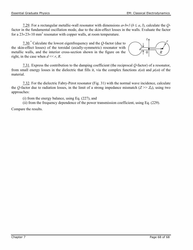
Essential Graduate Physics EM: Classical Electrodynamics
Chapter 7 Page 68 of 68
7.29. For a rectangular metallic-wall resonator with dimensions abl (b a, l), calculate the Q-factor in the fundamental oscillation mode, due to the skin-effect losses in the walls. Evaluate the factor for a 232310 mm3 resonator with copper walls, at room temperature. 7.30.* Calculate the lowest eigenfrequency and the Q-factor (due to the skin-effect losses) of the toroidal (axially-symmetric) resonator with metallic walls, and the interior cross-section shown in the figure on the right, in the case when d << r, R. 7.31. Express the contribution to the damping coefficient (the reciprocal Q-factor) of a resonator, from small energy losses in the dielectric that fills it, via the complex functions () and () of the material. 7.32. For the dielectric Fabry-Pérot resonator (Fig. 31) with the normal wave incidence, calculate the Q-factor due to radiation losses, in the limit of a strong impedance mismatch (Z >> Z0), using two approaches:
(i) from the energy balance, using Eq. (227), and (ii) from the frequency dependence of the power transmission coefficient, using Eq. (229).
Compare the results.
R
rz
0d