96

CHAPTER 7

CASE STUDIES

7.1 CASE STUDY ON OPTIMUM DESIGN SELECTION

THROUGH EVALUATION OF JIGS/FIXTURES USING

DIGRAPH AND MATRIX APPROACH

7.1.1 Introduction

Jig/fixture is an important element in any manufacturing process

that determines greater accuracy, efficiency and cost of machining, assembling

and inspection of products. Seldom a (it is hard to find) product is produced in

an industry that does not contain one or more holes. The location, finish and

size of these holes may be critical as in the case of a component for a missile.

In this way, the jigs/fixtures play an important role.

There are many jigs/fixtures for a component, which may vary in

their features based on the experience of the designer and there is no specific

methodology for the selection. So, selection (design) of an appropriate

jig/fixture for a component is not an easy task. Many authors suggested

various methods and techniques for the selection of jig/fixture, which are

detailed here. Kang et al. (2003) presented computer-aided fixture design

verification technique for verifying and improving the existing fixture designs.

Hurtado and Melkote (2002) presented a model for analysis of the effect of

fixture-workpiece conformability on static stability. Carlson (2001) used

kinematics analysis and derived a quadratic sensitivity equation that relates

position error in locators with the resulting displacement of the part held by

97

the locating scheme. Nee et al. (1987) reported the development of fixture

design procedure using artificial intelligence. In their research work, a

knowledge-based program structure was used to decide on an appropriate

fixture with respect to a particular workpiece specification. Qin et al. (2006)

presented a general analysis methodology that was able to characterise the

effects of localisation source errors based on the position and orientation of the

work piece. Wang et al. (2005) presented a method of fixturing error

measurement including component movement and component deflection. In

their research work, the error measurements in machined surfaces were used

for analysis and evaluation of fixture. Zheng (2005) in his PhD dissertation

established the finite element model of fixture for analyzing stiffness and

developed the experimental approaches to identify contact stiffness. Lin et al.

(2004) computed and analyzed the natural compliance of fixturing and

grasping arrangements. They derived a closed-form formula for the stiffness

matrix of multiple contact arrangements and used the same for investigating

the impact of different choices of contact model on the assessment of the

stability of multiple contact arrangements. Thus, many authors considered

various methods for the analysis and evaluation of jigs/fixtures, but no author

has reported the relative important between the attributes. Hence, a unique

selection method/procedure is much helpful in design stage.

Matrix and digraph approach is a logical approach and is applied by

various researchers (Venkata Rao R. and Gandhi O.P. 2002a, 2002b;

Ventaka Rao R, 2006a, 2006b; Sandeep Grover et al., 2004, 2005; Wani M.F

and Gandhi O.P 1999; Gandhi O.P. and Agrawal V.P. 1992; Sushma Kulkarni

2005; Garg et al., 2006). Specifically, the research works of Dr. Venkata Rao

motivated the author to use graph theory and matrix method for this problem.

In this section, matrix and digraph approach is used for the selection of

jig/fixture. The selection procedure includes the following phases:

98

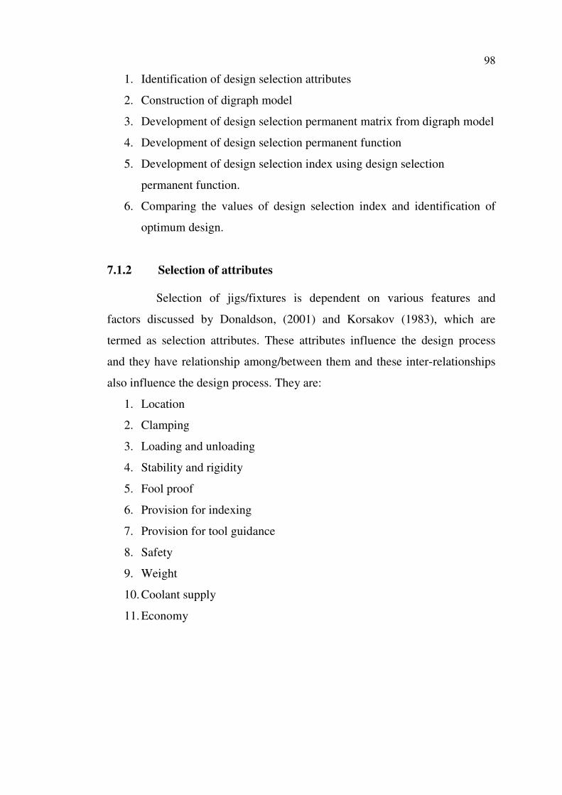
1. Identification of design selection attributes

2. Construction of digraph model

3. Development of design selection permanent matrix from digraph model

4. Development of design selection permanent function

5. Development of design selection index using design selection

permanent function.

6. Comparing the values of design selection index and identification of

optimum design.

7.1.2 Selection of attributes

Selection of jigs/fixtures is dependent on various features and

factors discussed by Donaldson, (2001) and Korsakov (1983), which are

termed as selection attributes. These attributes influence the design process

and they have relationship among/between them and these inter-relationships

also influence the design process. They are:

1. Location

2. Clamping

3. Loading and unloading

4. Stability and rigidity

5. Fool proof

6. Provision for indexing

7. Provision for tool guidance

8. Safety

9. Weight

10. Coolant supply

11. Economy

99

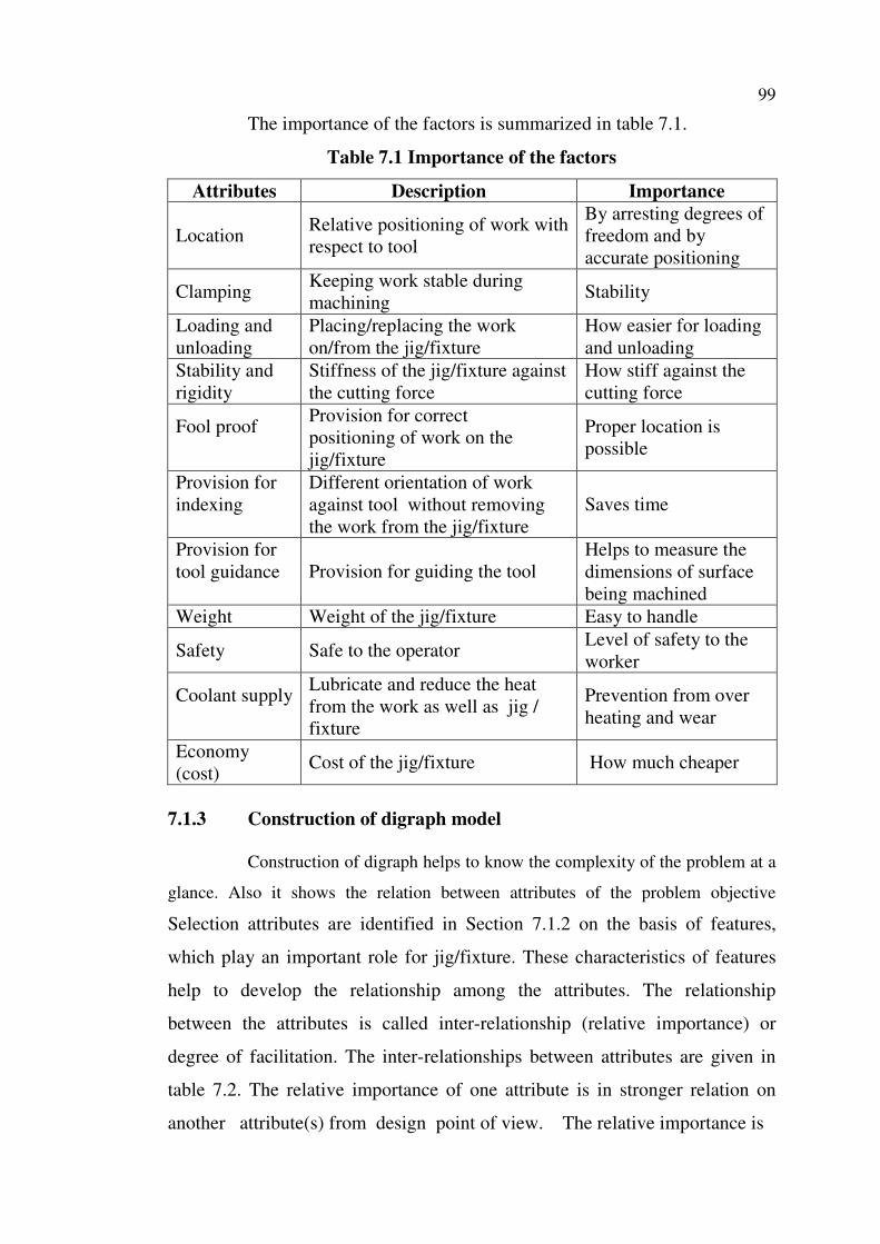
The importance of the factors is summarized in table 7.1.

Table 7.1 Importance of the factors

Attributes Description Importance

Location Relative positioning of work with

respect to tool

By arresting degrees of

freedom and by

accurate positioning

Clamping Keeping work stable during

machining Stability

Loading and

unloading

Placing/replacing the work

on/from the jig/fixture

How easier for loading

and unloading

Stability and

rigidity

Stiffness of the jig/fixture against

the cutting force

How stiff against the

cutting force

Fool proof

Provision for correct

positioning of work on the

jig/fixture

Proper location is

possible

Provision for

indexing

Different orientation of work

against tool without removing

the work from the jig/fixture

Saves time

Provision for

tool guidance

Provision for guiding the tool

Helps to measure the

dimensions of surface

being machined

Weight Weight of the jig/fixture Easy to handle

Safety Safe to the operator Level of safety to the

worker

Coolant supply

Lubricate and reduce the heat

from the work as well as jig /

fixture

Prevention from over

heating and wear

Economy

(cost) Cost of the jig/fixture How much cheaper

7.1.3 Construction of digraph model

Construction of digraph helps to know the complexity of the problem at a

glance. Also it shows the relation between attributes of the problem objective

Selection attributes are identified in Section 7.1.2 on the basis of features,

which play an important role for jig/fixture. These characteristics of features

help to develop the relationship among the attributes. The relationship

between the attributes is called inter-relationship (relative importance) or

degree of facilitation. The inter-relationships between attributes are given in

table 7.2. The relative importance of one attribute is in stronger relation on

another attribute(s) from design point of view. The relative importance is

100

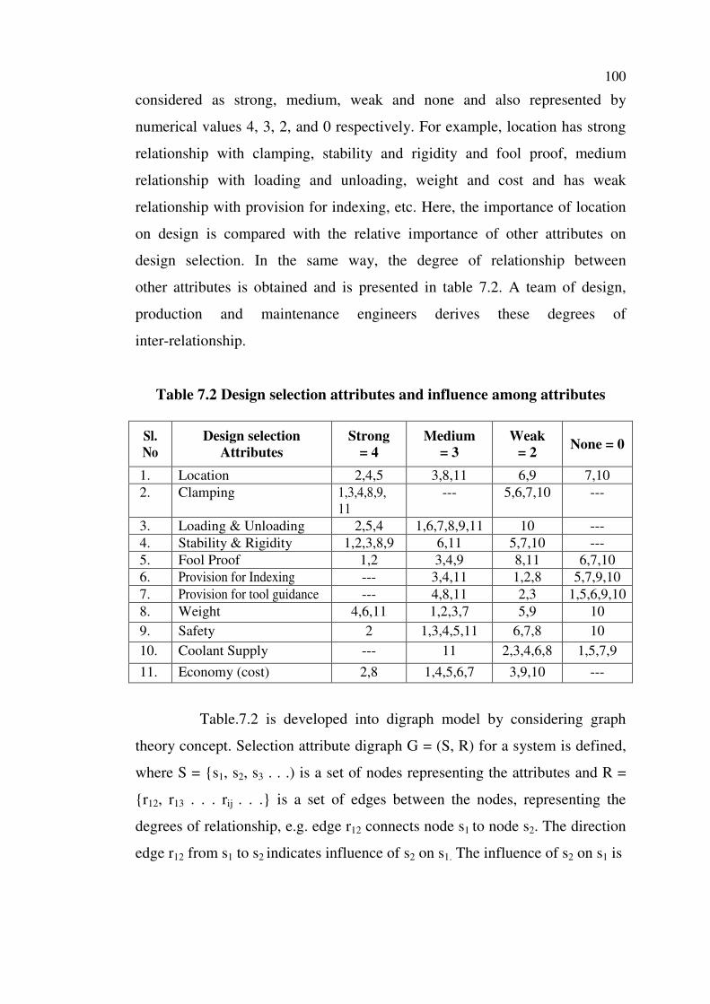
considered as strong, medium, weak and none and also represented by

numerical values 4, 3, 2, and 0 respectively. For example, location has strong

relationship with clamping, stability and rigidity and fool proof, medium

relationship with loading and unloading, weight and cost and has weak

relationship with provision for indexing, etc. Here, the importance of location

on design is compared with the relative importance of other attributes on

design selection. In the same way, the degree of relationship between

other attributes is obtained and is presented in table 7.2. A team of design,

production and maintenance engineers derives these degrees of

inter-relationship.

Table 7.2 Design selection attributes and influence among attributes

Sl.

No

Design selection

Attributes

Strong

= 4

Medium

= 3

Weak

= 2 None = 0

1. Location 2,4,5 3,8,11 6,9 7,10

2. Clamping 1,3,4,8,9,

11

--- 5,6,7,10 ---

3. Loading & Unloading 2,5,4 1,6,7,8,9,11 10 ---

4. Stability & Rigidity 1,2,3,8,9 6,11 5,7,10 ---

5. Fool Proof 1,2 3,4,9 8,11 6,7,10

6. Provision for Indexing --- 3,4,11 1,2,8 5,7,9,10

7. Provision for tool guidance --- 4,8,11 2,3 1,5,6,9,10

8. Weight 4,6,11 1,2,3,7 5,9 10

9. Safety 2 1,3,4,5,11 6,7,8 10

10. Coolant Supply --- 11 2,3,4,6,8 1,5,7,9

11. Economy (cost) 2,8 1,4,5,6,7 3,9,10 ---

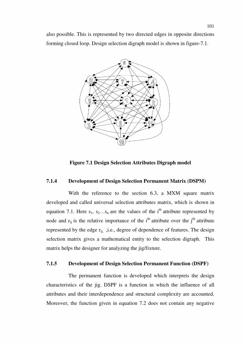
Table.7.2 is developed into digraph model by considering graph

theory concept. Selection attribute digraph G = (S, R) for a system is defined,

where S = {s1, s2, s3 . . .) is a set of nodes representing the attributes and R =

{r12, r13 . . . rij . . .} is a set of edges between the nodes, representing the

degrees of relationship, e.g. edge r12 connects node s1 to node s2. The direction

edge r12 from s1 to s2 indicates influence of s2 on s1. The influence of s2 on s1 is

101

also possible. This is represented by two directed edges in opposite directions

forming closed loop. Design selection digraph model is shown in figure-7.1.

Figure 7.1 Design Selection Attributes Digraph model

7.1.4 Development of Design Selection Permanent Matrix (DSPM)

With the reference to the section 6.3, a MXM square matrix

developed and called universal selection attributes matrix, which is shown in

equation 7.1. Here s1, s2…sn are the values of the ith

attribute represented by

node and rij is the relative importance of the ith

attribute over the jth

attribute

represented by the edge rij, ,i.e., degree of dependence of features. The design

selection matrix gives a mathematical entity to the selection digraph. This

matrix helps the designer for analyzing the jig/fixture.

7.1.5 Development of Design Selection Permanent Function (DSPF)

The permanent function is developed which interprets the design

characteristics of the jig. DSPF is a function in which the influence of all

attributes and their interdependence and structural complexity are accounted.

Moreover, the function given in equation 7.2 does not contain any negative

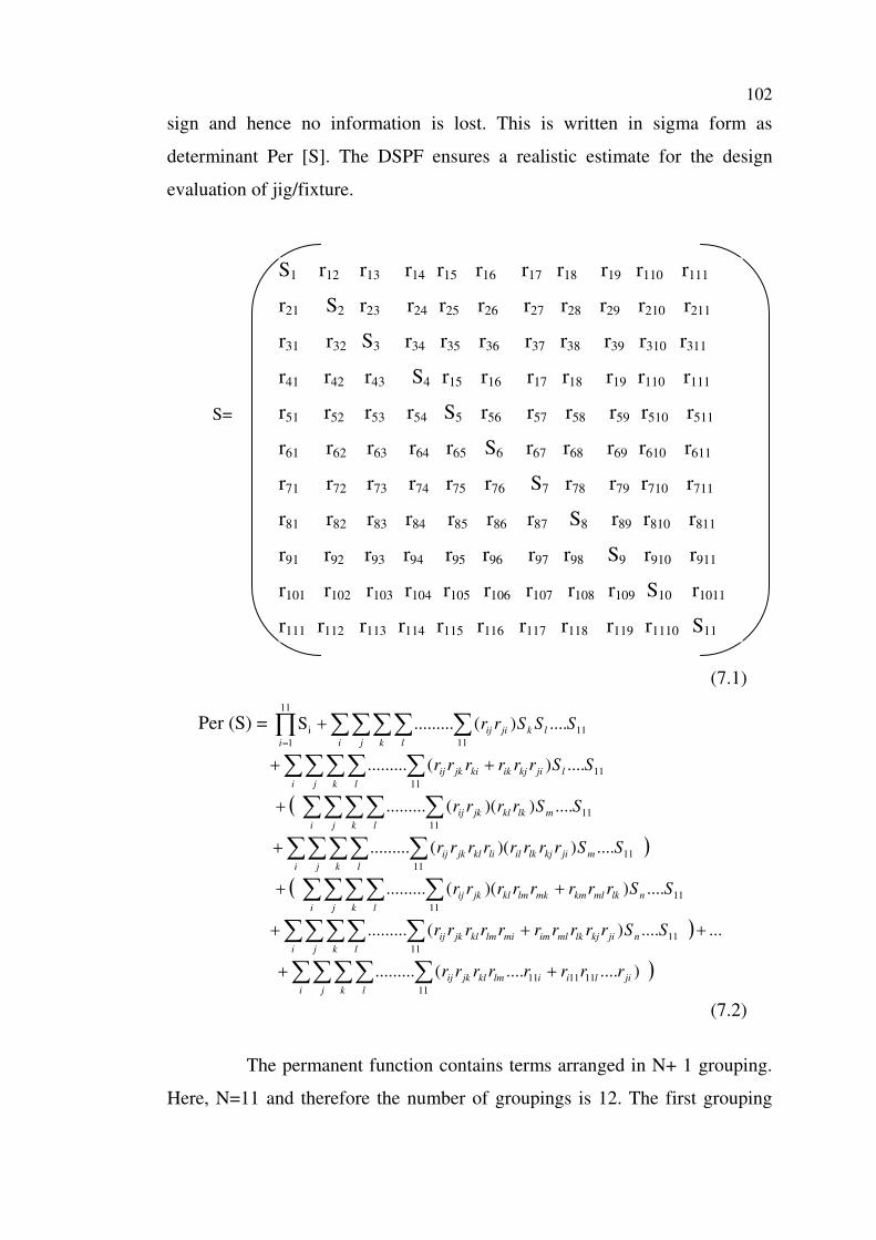
102

sign and hence no information is lost. This is written in sigma form as

determinant Per [S]. The DSPF ensures a realistic estimate for the design

evaluation of jig/fixture.

(7.1)

Per (S) = ∑∑∑∑ ∑∏ +

= i j

l

k

k

l

jiij

i

SSSrr 11

11

11

1

i ....)(.........S

∑∑∑∑ ∑ ++

i j k

ljikjikki

l

jkij SSrrrrrr 11

11

....)(.........

( ∑∑∑∑ ∑+

i j k

mlkkl

l

jkij SSrrrr 11

11

....))((.........

)∑∑∑∑ ∑+

i j k

mjikjlkillikl

l

jkij SSrrrrrrrr 11

11

....))((.........

( ∑∑∑∑ ∑ ++

i j k

nlkmlkmmklmkl

l

jkij SSrrrrrrrr 11

11

....))((.........

) .......)(......... 11

11

+++∑∑∑∑ ∑i j k

njikjlkmlimmilmkl

l

jkij SSrrrrrrrrrr

)∑∑∑∑ ∑ ++

i j k

jiliilmkl

l

jkij rrrrrrrr )........(......... 111111

11

(7.2)

The permanent function contains terms arranged in N+ 1 grouping.

Here, N=11 and therefore the number of groupings is 12. The first grouping

S1 r12 r13 r14 r15 r16 r17 r18 r19 r110 r111

r21 S2 r23 r24 r25 r26 r27 r28 r29 r210 r211

r31 r32 S3 r34 r35 r36 r37 r38 r39 r310 r311

r41 r42 r43 S4 r15 r16 r17 r18 r19 r110 r111

r51 r52 r53 r54 S5 r56 r57 r58 r59 r510 r511

r61 r62 r63 r64 r65 S6 r67 r68 r69 r610 r611

r71 r72 r73 r74 r75 r76 S7 r78 r79 r710 r711

r81 r82 r83 r84 r85 r86 r87 S8 r89 r810 r811

r91 r92 r93 r94 r95 r96 r97 r98 S9 r910 r911

r101 r102 r103 r104 r105 r106 r107 r108 r109 S10 r1011

r111 r112 r113 r114 r115 r116 r117 r118 r119 r1110 S11

S=

103

consists of only one term and is a set of design measures of N (11)

characteristics. In general, the second grouping is absent due to the absence

self loop in design selection digraph. The grouping represents a set of two

characteristics of self- loops in the design selection loops (i.e. rij rji ) and the

dependence of characteristic i and j and the design measure of N-2 (i.e.9

characteristics). Each term of the fourth grouping is a set of three

characteristic design loops, i.e. rij rjk rkl or its pair rik rkj rji and the design

measure of N-3, i.e. 8 characteristics. The terms of the fifth grouping are

arranged in two groupings. Each term of the first grouping is a set of two, two

characteristic design loops (i.e. rij rji and rkl rlk) and the design measure of N-4,

(i.e. 7 characteristics). Each term of the second grouping is a set of four

characteristic design loops, (i.e. rij rjk rkl rli or its pair ril rlk rkj rji,) and the design

measure of N-4, (i.e. 7 characteristics). The sixth grouping also contains two

sub groupings. The terms of the first sub grouping are a set of two

characteristic design loops, i.e. rij rji, a three characteristic design loop (i.e. rkl

rlm rmk or its pair rkm rml rlk) and design measures of N-5 (6 characteristics).

Each term of the second grouping is a five characteristic design loop (i.e. rij rjk

rkl rlm rmi or its pair rim rml rlk rkj rji) and the design measure of N-5 (i.e. 6

characteristics). Similarly, other terms of the function are defined. Each and

every term of the groupings and sub groupings has its own independent

identity.

7.1.6 Calculation of selection index using DSPF

Analysis for various designs for a jig is carried out in accordance

with the terms of DSPF, as it is the representation of the design selection. For

analysis purpose, its terms, which are considered as a set of distinct diagonal

elements (s1, s2…) and loops ( rij rjk … rqi) consist of off-diagonal matrix

elements. Each function leads to a useful test for analysis if a term is

interpreted as a set and not a dot product. There are N1 distinct ways in which

104

it can be formed from the design selection features. Based on this, selection of

design is carried out with respect to the terms appearing in its DSPF.

Design Selection Index (DSI)

DSPF becomes a useful tool to derive a quantitative measure/index

for the selection of jig/fixture. This index is known as a design selection index

(DSI). DSI is arrived from DSPF and it takes into account the values of

attributes and values for interrelationship between attributes. The index can be

evaluated if si and rij are assigned qualitative or quantitative values. These

values are assigned on appropriate scale. The values of interdependence given

in table 7.2 are arrived by a brainstorming session. The values of attributes are

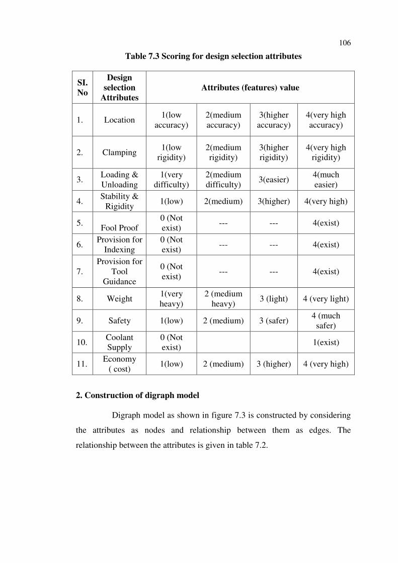
given in table 7.3. These values are assigned based on the understanding of the

features which may be normalized from 0-4/0-10. For the beneficial attributes,

the maximum values are given, if they are more desirable for the given

application. For example, 4 is given for very high accuracy location and 1 is

given for low accuracy location. Where non-beneficial attribute is one, the

lower value is desirable. For non beneficial attributes, value 4 is given as the

least desirable for the given application (for example- 4 is given for low

weight fixture and 1 is given for heavy weight fixture).

7.1.7 Selection of optimum design by comparison of DSI

DSI is a means to evaluate the various designs of Jig/ Fixture

through which an optimum design can be selected. This DSI is calculated for

all design varieties by assigning values in the function. Based on this value,

various designs of jig/fixture are arranged in ascending/descending order and a

design can be selected as optimum, whose DSI is larger.

105

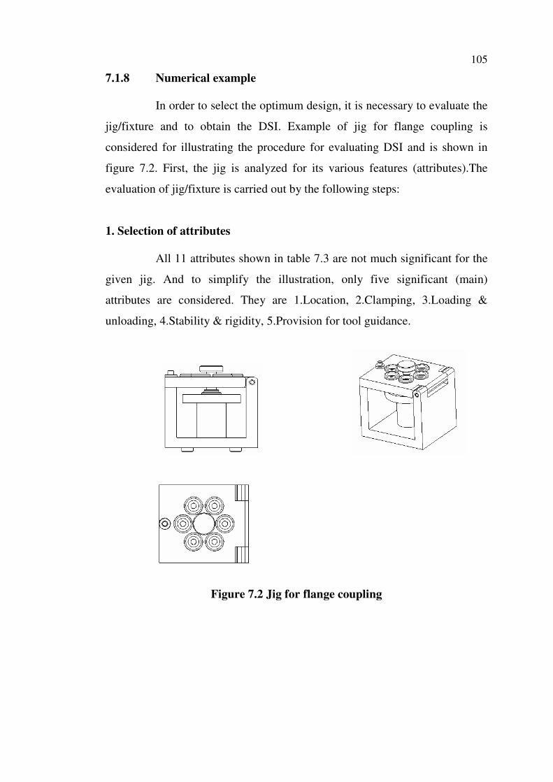
7.1.8 Numerical example

In order to select the optimum design, it is necessary to evaluate the

jig/fixture and to obtain the DSI. Example of jig for flange coupling is

considered for illustrating the procedure for evaluating DSI and is shown in

figure 7.2. First, the jig is analyzed for its various features (attributes).The

evaluation of jig/fixture is carried out by the following steps:

1. Selection of attributes

All 11 attributes shown in table 7.3 are not much significant for the

given jig. And to simplify the illustration, only five significant (main)

attributes are considered. They are 1.Location, 2.Clamping, 3.Loading &

unloading, 4.Stability & rigidity, 5.Provision for tool guidance.

Figure 7.2 Jig for flange coupling

106

Table 7.3 Scoring for design selection attributes

SI.

No

Design

selection

Attributes

Attributes (features) value

1. Location 1(low

accuracy)

2(medium

accuracy)

3(higher

accuracy)

4(very high

accuracy)

2. Clamping 1(low

rigidity)

2(medium

rigidity)

3(higher

rigidity)

4(very high

rigidity)

3. Loading &

Unloading

1(very

difficulty)

2(medium

difficulty) 3(easier)

4(much

easier)

4. Stability &

Rigidity 1(low) 2(medium) 3(higher) 4(very high)

5.

Fool Proof

0 (Not

exist) --- --- 4(exist)

6. Provision for

Indexing

0 (Not

exist) --- --- 4(exist)

7.

Provision for

Tool

Guidance

0 (Not

exist) --- --- 4(exist)

8. Weight 1(very

heavy)

2 (medium

heavy) 3 (light) 4 (very light)

9. Safety 1(low) 2 (medium) 3 (safer) 4 (much

safer)

10. Coolant

Supply

0 (Not

exist) 1(exist)

11. Economy

( cost) 1(low) 2 (medium) 3 (higher) 4 (very high)

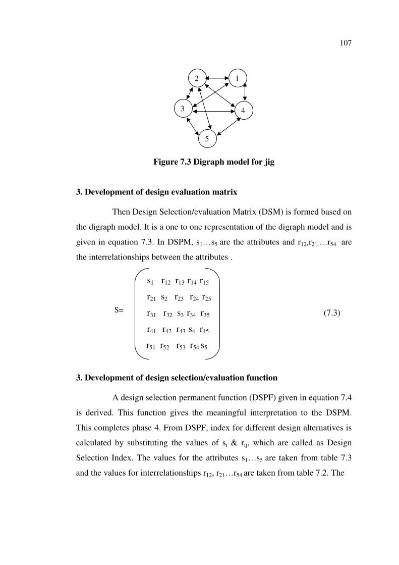
2. Construction of digraph model

Digraph model as shown in figure 7.3 is constructed by considering

the attributes as nodes and relationship between them as edges. The

relationship between the attributes is given in table 7.2.

107

Figure 7.3 Digraph model for jig

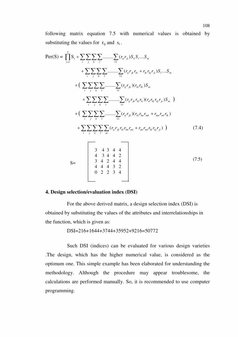
3. Development of design evaluation matrix

Then Design Selection/evaluation Matrix (DSM) is formed based on

the digraph model. It is a one to one representation of the digraph model and is

given in equation 7.3. In DSPM, s1…s5 are the attributes and r12,r21,…r54 are

the interrelationships between the attributes .

3. Development of design selection/evaluation function

A design selection permanent function (DSPF) given in equation 7.4

is derived. This function gives the meaningful interpretation to the DSPM.

This completes phase 4. From DSPF, index for different design alternatives is

calculated by substituting the values of si & rij, which are called as Design

Selection Index. The values for the attributes s1…s5 are taken from table 7.3

and the values for interrelationships r12, r21…r54 are taken from table 7.2. The

s1 r12 r13 r14 r15

r21 s2 r23 r24 r25

r31 r32 s3 r34 r35

r41 r42 r43 s4 r45

r51 r52 r53 r54 s5

S=

2

3

5

1

4

(7.3)

108

following matrix equation 7.5 with numerical values is obtained by

substituting the values for rij and si .

Per(S) = ∑∑∑∑ ∑∏ +

= i

m

j

l

k

k

l

jiij

i

SSSrr ....)(.........S11

5

1

i

∑∑∑∑ ∑ ++

i

m

j k

ljikjikki

l

jkij SSrrrrrr ....)(.........11

( ∑∑∑∑ ∑+

i j k

mlkkl

l

jkij Srrrr ))((.........11

)∑∑∑∑ ∑+

i j k

mjikjlkillikl

l

jkij Srrrrrrrr ))((.........11

( ∑∑∑∑ ∑ ++

i j k

lkmlkmmklmkl

l

jkij rrrrrrrr ))((.........11

)∑∑∑∑∑ ++

i j k

jikjlkmlimmilmkl

l

jk

m

ij rrrrrrrrrr )( (7.4)

4. Design selection/evaluation index (DSI)

For the above derived matrix, a design selection index (DSI) is

obtained by substituting the values of the attributes and interrelationships in

the function, which is given as:

DSI=216+1644+3744+35952+9216=50772

Such DSI (indices) can be evaluated for various design varieties

.The design, which has the higher numerical value, is considered as the

optimum one. This simple example has been elaborated for understanding the

methodology. Although the procedure may appear troublesome, the

calculations are performed manually. So, it is recommended to use computer

programming.

S=

3 4 3 4 4

4 3 4 4 2

3 4 2 4 4

4 4 4 3 2

0 2 2 3 4

(7.5)

109

7.2 ANALYSIS AND EVALUATION OF PRODUCT DESIGN

THROUGH DESIGN ASPECTS USING DIGRAPH AND

MATRIX APPROACH

7.2.1 Introduction

A successful product design fulfils the consumer’s needs. It is very

important for the designers to recognize these needs that go beyond the

utilitarian and functional to include the inspirational, emotional and cultural.

New product development also is indeed very important for manufacturers.

However, developing newer products is a risky and uncertain process. In order

to reduce the risks and uncertainties, companies need to evaluate their new

product initiatives carefully and make accurate decisions. This demonstrates

the increasing importance of the role of design both for economic

competitiveness and for improvement of the quality of life and work. One of

the major directions during the design process is that the products should

manifest end users point of view, from initial concept to their distribution to

the market place. Thus, product design evaluation is a must at all phases of the

product development process from concept phase to detailed design phase.

Design evaluation is time consuming and laborious, since many factors have

to be considered in relation to the development and design which vary in

character and complexity. Design evaluation cannot be made without

structured decision making tools (aids). Since the decision alternatives are too

many and simultaneous, criteria impact on the decision are too vast to consider

at once by human decision makers.

Maddulapalli A.K and Azarm S. (2006) addressed both kinds of

variability, i.e., variability in the preferences of the decision maker and

variability in the attribute levels of the design alternatives. They presented a

method for product design selection with variability in preferences for an

implicit value function and later extended it to account for variability in

attribute levels of design alternatives. Besharati B. et al. (2006) presented an

110

integrated design and marketing approach to facilitate the generation of an

optimal robust set of product design alternatives to carry forward to the

prototyping stage. Their approach evaluates the performance and robustness of

a design alternative due to variations in its uncontrollable parameters.

Vanegas V.L and Labib A.W. (2005) presented several fuzzy approaches to

design evaluation. Weight of criteria and performance levels are captured by

fuzzy numbers, and the overall performance of an alternative is calculated

through the new fuzzy weighted average.

Li H. and Azarm S. (2000) presented an approach wherein product

design is viewed as a selection process with two main stages: design

alternative generation and design alternative evaluation. The focus of their

paper was mainly on a design alternative evaluation model in which designer’s

preferences, customers’ preferences, and market competition are accounted for

the selection of the best possible design. See et al. (2004) discussed the

problem of selecting a design from a set of alternatives using multiple,

potentially conflicting criteria. They also demonstrated the strengths and

weaknesses of the various decision-making approaches using an aircraft

selection problem and then presented a method based on the concept of

hypothetical equivalents and expanded the method to include hypothetical in

equivalents. Ibusuki U. and Kaminski P.C. (2007) suggested a methodology

for the product development process in an automotive company, aiming at the

correct systematic approach of Value Engineering (VE) and target-costing in

cost management. Their proposed approach was validated in a case study

focused on the engine-starter system of a vehicle, aiming at improved product

cost, functionality and quality accomplishment, in accordance with customer

needs and the company strategy. Albritton M.P. and McMullen P.R. (2007)

suggested optimal product problem, where the “best” mix of product features

was formulated into an ideal offering and was optimized using Ant Colony

Optimization (ACO). Here, algorithm based on the behavior of social insects

111

was applied to a consumer decision model designed to guide new product

decisions and to allow planning and evaluation of product offering scenarios.

Chen L.H. and Weng M.L. (2006) suggested Quality Function

Deployment (QFD) to a product development process to achieve higher

customer satisfaction. The engineering characteristics affecting the product

performance are designed to match the customer requirements. Kim H.M.

et al. (2003) analyzed Automotive Vehicle Design by using Target Cascading,

a systematic effort to propagate the desired top-level system design targets to

appropriate specifications for subsystems and components in a consistent and

efficient manner. Many methodologies had been developed during the past

two decades by the academia and industry such as concurrent engineering,

robust design, design for manufacture and assembly, total quality

development, etc. Some other methods and techniques, which are used, are

given in the table 7.4.

Digraph and matrix approach has been used extensively by a

number of researchers in various engineering applications such as failure

cause analysis by Roa R.V et al. (2002), reliability evaluation by Sehgal R.

et al. (2000), proactive fault identification by Yu, Y et al. (2005), TQM

evaluation by Grover S. et al and Kulkarni S (2004, 2005), risk mitigation by

Faisal M.N et al. (2007) and in other areas also. Digraph and matrix approach

is a well systematic one, which considers all the influencing factors (attributes)

and their relative importance of one factor on the other. This consideration of

relative importance is missing in all other techniques discussed above. This

paper presents the analysis, evaluation and selection of product design through

design aspects using digraph and matrix approach.

112

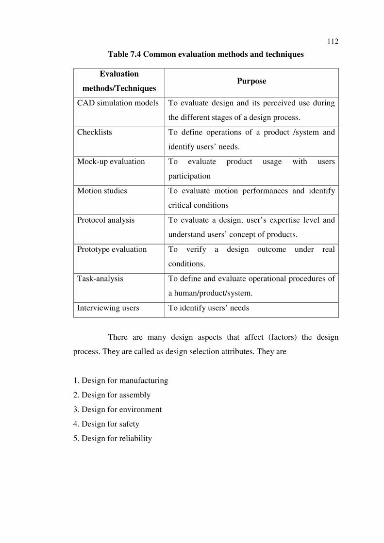
Table 7.4 Common evaluation methods and techniques

Evaluation

methods/Techniques Purpose

CAD simulation models To evaluate design and its perceived use during

the different stages of a design process.

Checklists To define operations of a product /system and

identify users’ needs.

Mock-up evaluation To evaluate product usage with users

participation

Motion studies To evaluate motion performances and identify

critical conditions

Protocol analysis To evaluate a design, user’s expertise level and

understand users’ concept of products.

Prototype evaluation To verify a design outcome under real

conditions.

Task-analysis To define and evaluate operational procedures of

a human/product/system.

Interviewing users To identify users’ needs

There are many design aspects that affect (factors) the design

process. They are called as design selection attributes. They are

1. Design for manufacturing

2. Design for assembly

3. Design for environment

4. Design for safety

5. Design for reliability

113

6. Design for maintenance

7. Design for aesthetic features

8. Design for economy

9. Design for ergonomics

The above said product design evaluation attributes are listed based

on the discussions in focus group (brain storming session) and from the

literatures [Otto K. and Wood K. (2000), Ulrich K.T. and Eppinger S.D.

(2008), Chitale A.K., Gupta R.C. (2001)]. A focus group is a collection of

individuals that has been brought together to discuss a particular topic, issue or

concern. This focus group technique as one approach enables the designer to

explore user desires and needs.

In general, these design aspects are innumerable and are referred to

as design for X (DFX) where X represents a broad variety of design

considerations which influence the design selection and are referred to as

design selection attributes. All these attributes and their importance on design

selection are explained in the forth coming section.

7.2.2 Product design evaluation attributes

a. Design for manufacturing (DFM)

DFM refers to the general engineering art of designing products in

such a way that they are easy to manufacture. The basic idea exists in almost

all engineering disciplines, but of course the details differ wildly depending on

the manufacturing technology. Traditionally, DFM method evaluates the

feasibility and cost of manufacturing of the product at the operation level.

Bralla J.G. (1986), Anderson D.M. (1990), Corbett J. et al. (1991), and

Boothroyd G. et al. (2002) provide detailed discussions on manufacturability

and design. Design guidelines such as those provided by Parmer C. and

114

Steve Laney (1993), Singh K. (1996), and Fagade A. and Kazmer D. (1998)

are examples of DFM method. As new DFX methods are explored, the

definition of DFM has expanded to become synonymous with DFX and

concurrent engineering. Various guidelines for DFM are given in the

appendix A.

b. Design for assembly (DFA)

DFA is a process by which products are designed with ease of

assembly in mind. If a product contains fewer parts, it will take less time to

assemble, thereby reducing assembly costs. In addition, if the parts are

provided with features, which make it easier to grasp, move, orient and insert

them, assembly time and assembly costs reduce. DFA guidelines adapted from

several sources such as Andreasen D.M. (1983), Baldwin S. (1996), Huthwaite

B. (1990), Iredale R. (1964) and Xerox (1986). DFM and DFA are most of the

time considered simultaneously as DFMA(design for manufacturing and

assembly). But, they have conflicting nature among them. DFMA is important

for design because it has three beneficial impacts. First and foremost, it

reduces part count and also reduces cost and time. For example, Motorola

introduced DFMA and reduced its part count from 217 to 97 and there by

assembly time is reduced from 2,700 to 1,350 s [Otto K., Wood K.(2000)].

Secondly, DFMA increases reliability [Bralla J.G. (1991), Barkan P., Hinckley

C. (1993)]. Finally, DFMA increases the quality of the design. Various

guidelines for the DFA are given in appendix B.

c. Design For Environment (DFE)

The present problem of global warming is a challenging one for the

manufacturing industries. DFE is a product design approach for reducing the

impact of the products on the environment. Products can have adverse impact

on the environment during manufacturing through the use of highly polluting

115

processes and consumption of large quantities of raw materials and energy and

disposal of waste. Because of these issues, one must consider the entire life

cycle of the product from creation to disposal. In this life cycle, there are many

events of creating pollution and many opportunities for recycling,

remanufacturing, reuse, and reducing environmental impact. Designer must

bring all his ingenuity to keep in mind all the challenging problems while

creating efficient products. Various guidelines for the DFE are given in

appendix C.

d. Design for Safety(DFS)

The goals of the design process are usually manifold. The resulting

system must not only satisfy its functional requirements but also have to fulfill

certain non-functional requirements. One such requirement is safety. A safe

product is one that does not cause injury or property loss and does not pollute

the environment. There are three aspects to design for safety.

1. Make the product safe.

2. If it is not possible to make the product inherently safe, then design the

proactive devices like guards, automatic cutoff switches, pressure relief

valves, to mitigate the hazard.

3. If step 2 cannot remove all the hazards, then warn the user of the product

with appropriate warnings like labels, flashing and loud sounds. Various

guidelines for the design for safety are given in appendix D.

e. Design for Reliability(DFR)

Reliability engineering is the discipline of ensuring that a system

will be reliable when operated in a specified manner. Reliability engineering is

performed throughout the entire life cycle of a system, including development,

test, production and operation. Reliability may be defined in several ways as:

116

• Idea that something is fit for a purpose with respect to time.

• Capacity of a device or system to perform as designed.

• Resistance to failure of a device or system.

• Ability of a device or system to perform a required function under

stated conditions for a specified period of time.

• Probability that a functional unit will perform its required function for a

specified interval under stated conditions.

Reliability engineers rely heavily on statistics, probability theory,

and reliability theory. Many engineering techniques are used in reliability

engineering, such as reliability prediction, Weibull analysis, thermal

management, reliability testing and accelerated life testing. Because of the

large number of reliability techniques, their expense, and the varying degrees

of reliability required for different situations, most of the projects develop a

reliability program plan to specify the reliability tasks that will be performed

for that specific system. Various guidelines for the design for reliability are

given in the appendix E.

f. Design for Maintenance (Serviceability) (DFMn)

Serviceability is concerned with the ease with which maintenance

can be performed on a product. Products often have parts that are to be

replaced at periodic intervals. It is important to anticipate the required service

operations during the design of the product. Provision must be made for

disassembly and assembly. For example, don’t make an automobile design

that requires the removal of the panel to access the oil filter. Also, remember

that service usually will be carried out in “the field” where special tools and

fixtures used in factory assembly are not available. The best way to improve

serviceability is to reduce the need for service by improving reliability of the

117

components and systems. Various guidelines for the design for maintenance

are given in appendix F.

g. Design for Aesthetic Features(DFAF)

Designers have many aesthetic qualities to improve the

marketability of the manufactured products: smoothness, shine/reflectivity,

texture, pattern, curviness, color, simplicity, usability, velocity, symmetry,

naturalness, and modernism. The staff of the design aesthetics section focus on

design, appearance and the way people perceives products. Design aesthetics

is interested in the appearance of products; the meaning of appearance is

studied mainly in terms of social and cultural factors. The distinctive focus of

the section is research and education in the field of sensory modalities in

relation to product. These fields of attention generate design baggage that

enables engineers to design products, systems, and services, and match them

to the correct field of use. Various guidelines for the design of aesthetic

features are given in appendix G.

h. Design for Economy (DFEc)

It is important to note that cost is also a dimension of the quality.

Economically successful products are profitable; that is, they generate more

cumulative inflows than the cumulative outflows. The main objective of all

manufacturers is to make profit. So, the producer should give a cost effective

design. Based on the cost and other considerations, the designer should select

material or manufacturing processes. Various guidelines for the design for

economy are given in appendix H.

118

i. Design for Ergonomics(DFEr)

Ergonomics (or human factors) is the application of scientific

information concerning humans to the design of objects, systems and

environment for human use. (Definition adopted by the International

Ergonomics Association in 2007). Ergonomics is the study of the interaction

of a person with a machine. Information derived from Ergonomists

contributes to the design and evaluation of tasks, jobs, products, environments

and systems in order to make them compatible with the needs, abilities and

limitations of people (International Ergonomics Association in 2000).

Ergonomics comes into everything, which involves people. Work systems,

sports and leisure, health and safety should all embody ergonomics principles

if well designed. (International Ergonomics Association in 2007). It is the

applied science of equipment design intended to maximize productivity by

reducing operator fatigue and discomfort. The field is also called

biotechnology, human engineering, and human factors engineering. The role

of human factors in a product assumes importance in three respects.

1. Man, the operator, as occupant of space that is to operate a machine,

should have adequate space as dictated by human body dimensions or

anthropometry.

2. Man, as reader of display from the machine. This is based on the

display data; man processes the data and takes action.

3. Man, as one who takes action through operating controls which form a

part of the machine. It will be obvious that human engineering in

design should consider application of forces and study of displays and

controls.

Various guidelines for the design for ergonomics are given in the

appendix I. Design for X (DFX), where X corresponds to one of dozens of

quality criteria, which are listed earlier. This list is not an exhaustive one and

119

the same may be extended further for dozens of criteria. They may be

specifically related to the product or processes. For example, design for

handling, design for flow ability (casting process), design for recycle ability,

design for remanufacturing, design for energy efficiency and design for

regulations and standards, etc.

7.2.3 Product design Evaluation Digraph (PED) model

A digraph is used to represent the factors and their inter

dependences in terms of nodes and edges. In a digraph, direction is assigned to

edges in the graph. Thus, product design evaluation attributes’ digraph

consists of set of nodes, S = {Pi } with i = 1, 2. . ., M and set of edges, E = {ri j

}. A node Pi represents ith

product design evaluation attribute and the rij edge

represents relative importance among the attributes. The number of nodes M is

equal to the number of product design evaluation attributes considered for the

selection of design. If a node i has relative importance over another node j in

the selection, then, a directed edge (arrow) is drawn from node i to j (i.e., rij ).

If j has relative importance over i, then the directed edge (arrow) is drawn

from node j to i (i.e., r ji ). The most common representation of a graph is a

diagram in which the vertices are represented as points and edges as line

segments joining the end vertices. A universal product evaluation digraph

model is constructed as shown in figure 7.4 by considering the attributes

described in section 7.2.2 as nodes and the relative importance between the

attributes as edges.

120

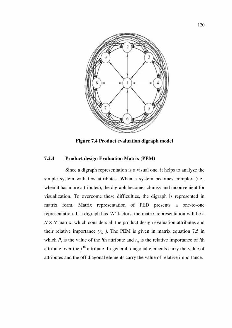
Figure 7.4 Product evaluation digraph model

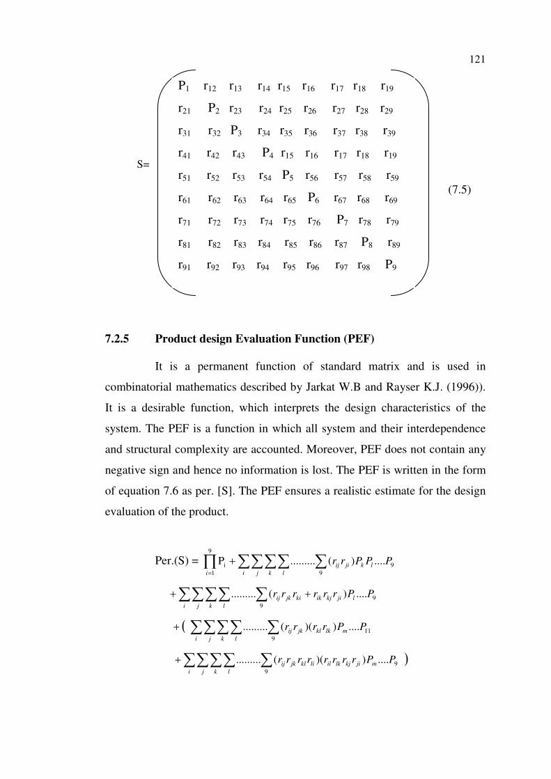
7.2.4 Product design Evaluation Matrix (PEM)

Since a digraph representation is a visual one, it helps to analyze the

simple system with few attributes. When a system becomes complex (i.e.,

when it has more attributes), the digraph becomes clumsy and inconvenient for

visualization. To overcome these difficulties, the digraph is represented in

matrix form. Matrix representation of PED presents a one-to-one

representation. If a digraph has ‘N’ factors, the matrix representation will be a

N × N matrix, which considers all the product design evaluation attributes and

their relative importance (rij ). The PEM is given in matrix equation 7.5 in

which Pi is the value of the ith attribute and rij is the relative importance of ith

attribute over the j th

attribute. In general, diagonal elements carry the value of

attributes and the off diagonal elements carry the value of relative importance.

121

7.2.5 Product design Evaluation Function (PEF)

It is a permanent function of standard matrix and is used in

combinatorial mathematics described by Jarkat W.B and Rayser K.J. (1996)).

It is a desirable function, which interprets the design characteristics of the

system. The PEF is a function in which all system and their interdependence

and structural complexity are accounted. Moreover, PEF does not contain any

negative sign and hence no information is lost. The PEF is written in the form

of equation 7.6 as per. [S]. The PEF ensures a realistic estimate for the design

evaluation of the product.

Per.(S) = ∑∑∑∑ ∑∏ +

= i j

l

k

k

l

jiij

i

PPPrr 9

9

9

1

i ....)(.........P

∑∑∑∑ ∑ ++

i j k

ljikjikki

l

jkij PPrrrrrr 9

9

....)(.........

( ∑∑∑∑ ∑+

i j k

mlkkl

l

jkij PPrrrr 11

9

....))((.........

)∑∑∑∑ ∑+

i j k

mjikjlkillikl

l

jkij PPrrrrrrrr 9

9

....))((.........

P1 r12 r13 r14 r15 r16 r17 r18 r19

r21 P2 r23 r24 r25 r26 r27 r28 r29

r31 r32 P3 r34 r35 r36 r37 r38 r39

r41 r42 r43 P4 r15 r16 r17 r18 r19

r51 r52 r53 r54 P5 r56 r57 r58 r59

r61 r62 r63 r64 r65 P6 r67 r68 r69

r71 r72 r73 r74 r75 r76 P7 r78 r79

r81 r82 r83 r84 r85 r86 r87 P8 r89

r91 r92 r93 r94 r95 r96 r97 r98 P9

S=

(7.5)

122

( ∑∑∑∑ ∑ ++

i j k

nlkmlkmmklmkl

l

jkij PPrrrrrrrr 9

9

....))((.........

) .......)(......... 9

9

+++∑∑∑∑ ∑i j k

njikjlkmlimmilmkl

l

jkij PPrrrrrrrrrr

)∑∑∑∑ ∑ ++

i j k

jiliilmkl

l

jkij rrrrrrrr )........(......... 111111

9

(7.6)

The product design evaluation function Per.(S) contains terms

arranged in (M + 1) groupings and these groupings represent the presence of

attributes and the relative importance loops. The first grouping represents the

presence of all product design attributes. In general, the second grouping is

absent due to the absence self loop in product design attributes digraph. The

third grouping contains 2-attributes relative importance loops and the presence

of (M −2) attributes. Fourth grouping represents a set of 3-attributes relative

importance loops or its pairs and presence of (M − 3) attributes. The fifth

grouping contains two sub-groupings. The terms of the first sub-grouping are a

set of two 2- attributes relative importance loops and the presence of (M−4)

attributes. Each term of the second sub-grouping is a set of 4-attributes relative

importance loops or its pairs and the presence of (M − 4) attributes. The sixth

grouping contains two sub-groupings. The terms of the first sub-grouping are a

set of 2-attribues relative importance loops and 3 attributes relative importance

loops or its pairs and presence of (M − 5) attributes. The term of second sub-

grouping is a 5- attributes relative importance loop or its pairs and the

presence of (M −5) attributes. Similarly, other terms of the expression are

defined. Thus, product design evaluation function characterizes the product

design as it contains all attributes and their relative importance.

7.2.6 Product design Evaluation Index(PEI)

PEI is a numerical value that defines the overall effectiveness of the

product design with respect to design aspects and provides the information of

the product design with respect to customer satisfaction. PEI is obtained from

123

the product design evaluation function (equation 7.6) by substituting the

values of attributes Pi and the values of relative importance between the

attributes r ij . The values for attributes Pi are obtained from the data provided

by the industries and expertise. The value of many attributes cannot be

expressed as numerical values. If a quantitative value is not available, then a

ranked value judgment on a scale, e.g., from 0 to 10 scales, is adopted. It is

seen that many of the attributes are not easy to measure in terms of qualitative

scale. Hence, a questionnaire has been designed to measure each attribute in

terms of weightage (questionnaire is given in appendix). The numerical values

obtained through questionnaire are normalized on the same scale, i.e., 0–10. If

Pi has a range Pil and Piu, the value 0 is assigned to the lowest range value

(Pil ) and 10 is assigned to the highest range value (Piu). The other intermediate

values Pi of the product design attribute are assigned values between 0 and 10

as follows:

Pi = {10/ Piu } × Pii for Pil = 0

Pi = {10/( Piu − Pil )} × (Pii − Pil ) for Pil >0 (7.7)

Equation 7.7 is applicable for general beneficial attributes only. A

beneficial attribute i.e., design for safety, means its higher attribute values are

more desirable for the given product design, whereas a non beneficial attribute

i.e., design for economy is one for which lower attribute values are desirable.

Therefore, in case of non beneficial product design attributes, the value 0 and

10 are assigned to the highest range value (Piu) and the lowest range value (Pil

) respectively. The other intermediate values Pii of the product design attribute

are assigned between 0 and 10 as follows:

Pi = 10{1 − (Pii /Piu)} for Pil = 0

Pi = {10/(Piu − Pil )} × (Piu − Pii ) for Pil >0 (7.8)

124

For example, the attribute design for safety with the higher value is

much safer to use. So, the value for the attribute design for safety with higher

value is beneficial to customers as well as manufacturers. So, the quantitative

value obtained from the appendix for DFS is substituted in equations 7.7 for

normalizing. On the other hand, the attribute design for economy means total

cost of the product involved in product development. If the total cost is higher,

both the customer and the manufacturer will not be benefited. So, the attribute

DFE is considered as non-beneficial attribute and it should have minimum

value. So, the value obtained from appendix for DFE is substituted in equation

7.8 for normalizing.

The relative importance between the two attributes (i.e., rij) for a

given product design is also assigned a value on the scale 0–10 and is arranged

in six classes. The relative importance implies that an attribute ‘i’ is compared

with another attribute ‘j’ in terms of its relative importance for the given

product design. The relative importance between i, j and j i is distributed on

the scale 0–10. This means, a scale is adopted from 0 to 10 on which the

relative importance values are compared. If rij represents the relative

importance of the ith attribute over the j th attribute, then the relative

importance of the j th attribute over the ith attribute is evaluated using

equation rji=10-rij. For example, if j th attribute is slightly more important than

the ith attribute, then rji = 6 and rij = 4. Comparative scale for assigning the

vales of rij and rji is given in the table 7.5. The product design evaluation index

value for all design alternatives is evaluated by substituting the values of Pi’s

and rij’s in equation7.6. The product designs can be arranged in the descending

or ascending order of PEI, to rank them for their performance. The product

design, for which the value of PEI is highest, is considered to be the best. The

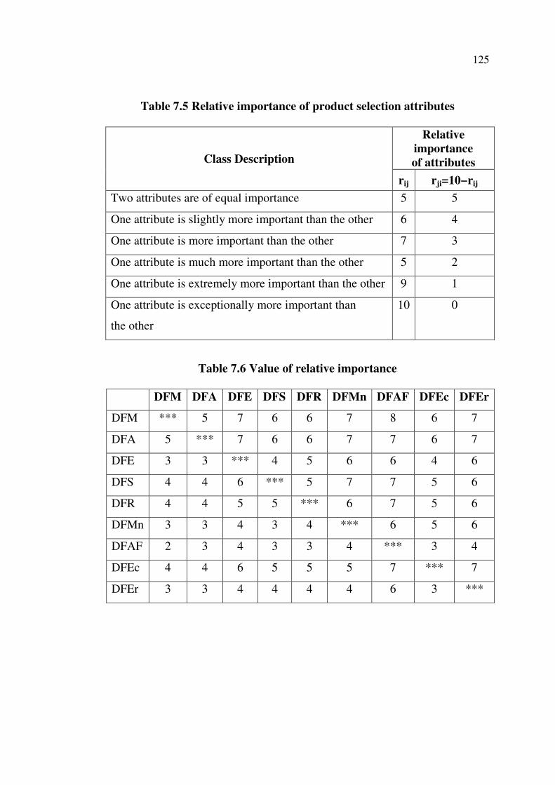
value of the relative importance between the attributes is assigned based on

table 7.5 and is given in table 7.6.

125

Table 7.5 Relative importance of product selection attributes

Relative

importance

of attributes Class Description

rij rji=10−rij

Two attributes are of equal importance 5 5

One attribute is slightly more important than the other 6 4

One attribute is more important than the other 7 3

One attribute is much more important than the other 5 2

One attribute is extremely more important than the other 9 1

One attribute is exceptionally more important than

the other

10 0

Table 7.6 Value of relative importance

DFM DFA DFE DFS DFR DFMn DFAF DFEc DFEr

DFM *** 5 7 6 6 7 8 6 7

DFA 5 *** 7 6 6 7 7 6 7

DFE 3 3 *** 4 5 6 6 4 6

DFS 4 4 6 *** 5 7 7 5 6

DFR 4 4 5 5 *** 6 7 5 6

DFMn 3 3 4 3 4 *** 6 5 6

DFAF 2 3 4 3 3 4 *** 3 4

DFEc 4 4 6 5 5 5 7 *** 7

DFEr 3 3 4 4 4 4 6 3 ***

126

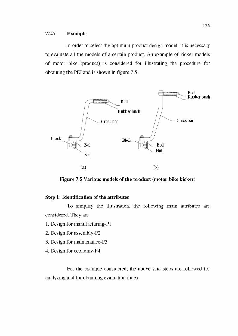
7.2.7 Example

In order to select the optimum product design model, it is necessary

to evaluate all the models of a certain product. An example of kicker models

of motor bike (product) is considered for illustrating the procedure for

obtaining the PEI and is shown in figure 7.5.

(a) (b)

Figure 7.5 Various models of the product (motor bike kicker)

Step 1: Identification of the attributes

To simplify the illustration, the following main attributes are

considered. They are

1. Design for manufacturing-P1

2. Design for assembly-P2

3. Design for maintenance-P3

4. Design for economy-P4

For the example considered, the above said steps are followed for

analyzing and for obtaining evaluation index.

127

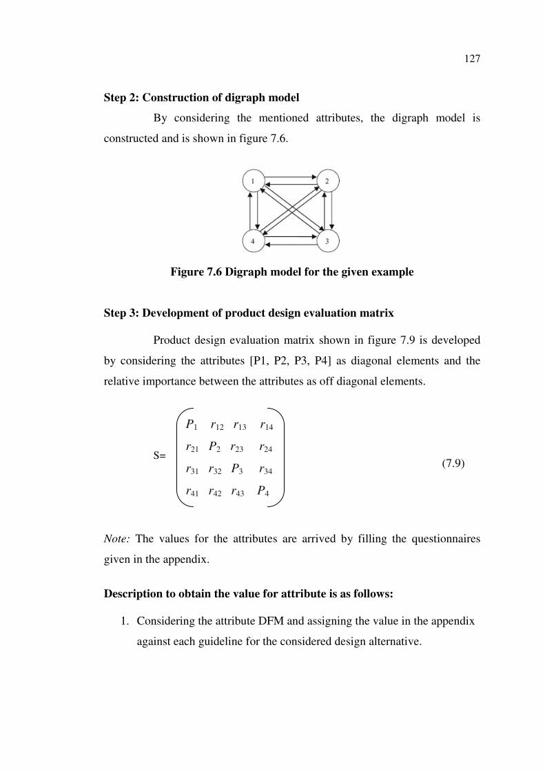
Step 2: Construction of digraph model

By considering the mentioned attributes, the digraph model is

constructed and is shown in figure 7.6.

Figure 7.6 Digraph model for the given example

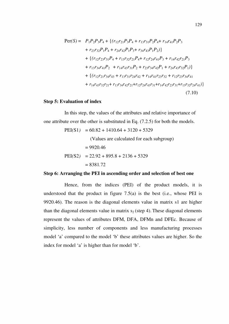
Step 3: Development of product design evaluation matrix

Product design evaluation matrix shown in figure 7.9 is developed

by considering the attributes [P1, P2, P3, P4] as diagonal elements and the

relative importance between the attributes as off diagonal elements.

(7.9)

Note: The values for the attributes are arrived by filling the questionnaires

given in the appendix.

Description to obtain the value for attribute is as follows:

1. Considering the attribute DFM and assigning the value in the appendix

against each guideline for the considered design alternative.

P1 r12 r13 r14

r21 P2 r23 r24

r31 r32 P3 r34

r41 r42 r43 P4

S=

128

2. Assigning the minimum possible value for the each guide lines of DFM

and summing up all the values and assuming as the Pil (lower value of

the ith attribute). For this example Pil = 25.

3. Assigning the maximum possible value for the each guide lines of

DFM and summing up all the values and assuming as the Piu (higher

value of the ith attribute). For this example, Piu = 115

4. Assigning the value for each guide lines of DFM of the considered

product design and summing up all the values and assuming as Pii

(value of the attribute of the considered product design) For the product

design given in figure.7.5, Pii = 65

5. Substituting this value in the equation 7.7 to get the normalized value

on 0–10 scale.

Pi = {10/(Piu − Pil )} × (Pii − Pil ) for Pil > 0

= {10/(115 − 25)} × (65 − 25)

= 0.111 × 40 = 4.4

Similarly, the other attribute values are normalized.

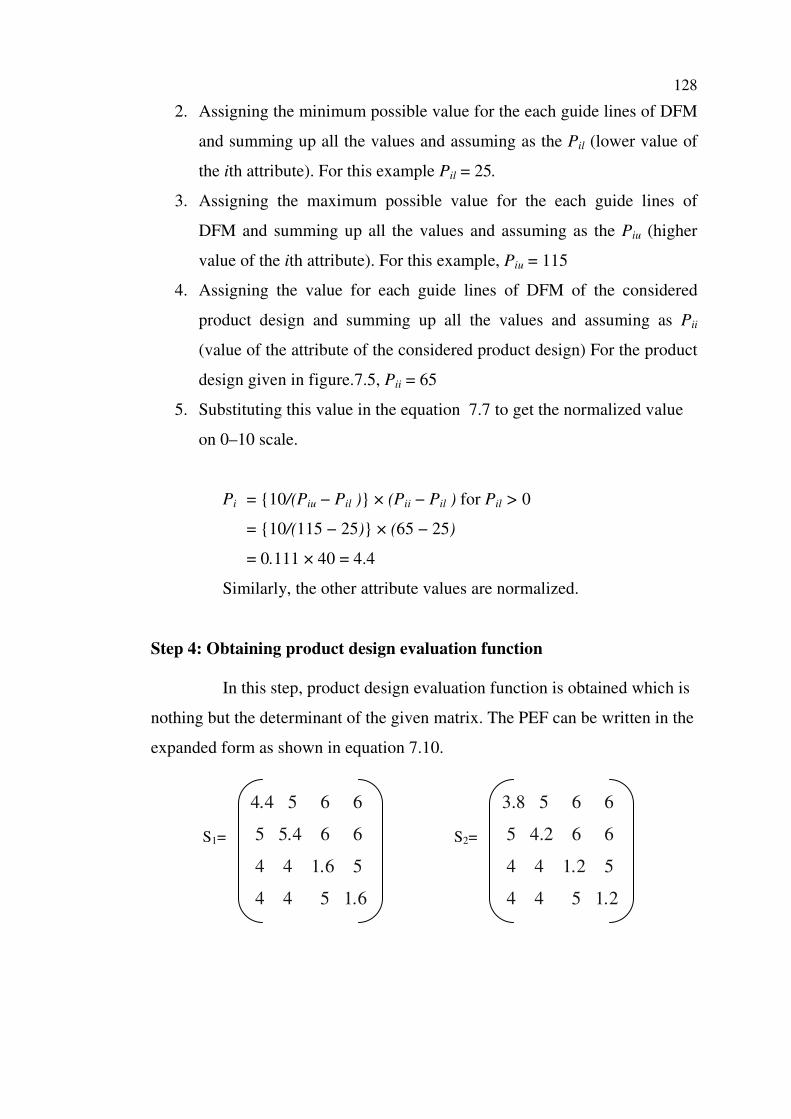
Step 4: Obtaining product design evaluation function

In this step, product design evaluation function is obtained which is

nothing but the determinant of the given matrix. The PEF can be written in the

expanded form as shown in equation 7.10.

4.4 5 6 6

5 5.4 6 6

4 4 1.6 5

4 4 5 1.6

S1=

3.8 5 6 6

5 4.2 6 6

4 4 1.2 5

4 4 5 1.2

S2=

129

Per(S) = P1P2P3P4 + {(r12r21P3P4 + r13r31P2P4+ r14r41P2P3

+ r23r32P1P4 + r24r42P1P3+ r34r43P1P2)}

+ {(r12r23r31P4 + r13r32r21P4+ r12r24r41P3 + r14r42r21P3

+ r13r34r41P2 + r14r43r31P2 + r23r34r42P1 + r24r43r32P1)}

+ {(r12r21r34r43 + r13r31r24r42 + r14r41r23r32 + r12r23r34r41

+ r14r43r32r21+ r13r34r42r21+r12r24r43r31+r14r42r23r31+r13r32r24r41)}

(7.10)

Step 5: Evaluation of index

In this step, the values of the attributes and relative importance of

one attribute over the other is substituted in Eq. (7.2.5) for both the models.

PEI(S1) = 60.82 + 1410.64 + 3120 + 5329

(Values are calculated for each subgroup)

= 9920.46

PEI(S2) = 22.92 + 895.8 + 2136 + 5329

= 8381.72

Step 6: Arranging the PEI in ascending order and selection of best one

Hence, from the indices (PEI) of the product models, it is

understood that the product in figure 7.5(a) is the best (i.e., whose PEI is

9920.46). The reason is the diagonal elements value in matrix s1 are higher

than the diagonal elements value in matrix s2 (step 4). These diagonal elements

represent the values of attributes DFM, DFA, DFMn and DFEc. Because of

simplicity, less number of components and less manufacturing processes

model ‘a’ compared to the model ‘b’ these attributes values are higher. So the

index for model ‘a’ is higher than for model ‘b’.