Chapter 66

Of Mice and Men: Algorithms for Evolutionary Distances Between Genomes with Translocation

John D. Kececioglut R. Ravi*

Abstract

A new and largely unexplored area of computational biology is combinatorial algorithms for genome rear- rangement. In the course of its evolution, the genome of an organism mutates by processes that can rear- range whole segments of a chromosome in a single event. These rearrangement mechanisms include in- version, transposition, duplication, and translocation, and a basic problem is to determine the minimum number of such events that transform one genome to another. This number is called the rearrangement dis- tance between the two genomes, and gives a lower bound on the number of events that must have oc- curred since their divergence, assuming evolution pro- ceeds according to the processes of the study.

In this paper, we begin the algorithmic study of genome rearrangement by translocation. A transloca- tion exchanges material at the end of two chrome somes within a genome. We model this as a pro- cess that exchanges prefixes and suffixes of strings, where each string represents a sequence of distinct markers along a chromosome in the genome. For the general problem of determining the translocation dis- tance between two such sets of strings, we present a 2-approximation algorithm. For a theoretical model in which the exchanged sub&rings are of equal length, we derive an optimal algorithm for translocation dis- tance.

We also examine for the first time two types of rearrangements in concert. An inversion reverses the order of markers within a substring, and flips the

‘work carried out while the authors were at the Department of Computer Science of the University of California, Davis.

iDepartment of Computer Science, The University of Geor- gia, Athens, GA 30602. Electronic mail: kecoQcs.uga.sdu. This research was supported by a DOE Human Genome Dis- tinguished Postdoctoral Fellowship.

tDepartment of Computer Science, Princeton University, Princeton, NJ 08544. Electronic mail: ravi@cs .prinoeton. l du. Research supported by DOE Grant DEFG03-90ER60999 and a DIMACS Postdoctoral Fellowship.

orientation of the markers. For genomes that have evolved by translocation and inversion, we show there is a simple 2-approximation algorithm for data in which the orientation of markers is unknown, and a $- approximation algorithm when orientation is known.

These results take a step towards extending the area from the analysis of simple organisms, whose genomes consist of a single chromosome, and whose evolution has largely involved a single type of rear- rangement event, to the analysis of organisms such as man and mouse, whose genomes contain many chromosomes, and whose history since divergence has largely consisted of inversion and translocation events.

1 Introduction and motivation

Molecular biology is entering a new era in which data will soon become available on the entire complement of DNA, known as the genome, of man and model or- ganisms such the mouse [4]. Genomes of these and other complex organisms are organized into chromo- somes, which contain the genes of the organism ar- ranged in a linear order. Much of the current data for genomes is in the form of maps, which identify the location of genes and other markers of interest along the chromosomes. Maps are now becoming available that show the location of markers common to both man and mouse [lo], and such data permits for the first time the study of the evolution of such organisms at the scale of the genome [9].

In contrast to evolution at the level of individ- ual genes, which proceeds by local operations, such as point mutation, which substitutes, inserts, and deletes individual letters of the DNA sequence, evolution at the level of the genome proceeds by non-local, large- scale operations, which can rearrange a whole seg- ment of the chromosome in one evolutionary event. These non-local operations include: inversion, which replaces a segment of a chromosome with its reverse

604

EVOLUTIONARY DISTANCES WITH TRANSLOCATION 605

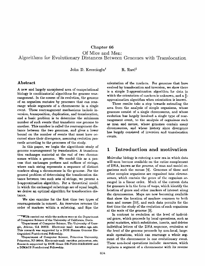
Figure 1 An example of a translocation between two chromosomes. A segment from the end of each chromo- some is exchanged.

DNA sequence, and has the effect of reversing the or- der and orientation of markers within the segment; trawposition, which moves a segment to a new loca- tion in the genome; duplication, which copies a seg- ment to a new location; and ban&cation, which ex- changes segments between the ends of two chromo- somes (see Figure 1). Such large-scale rearrangements occur at a much slower rate than point mutations, and are now a subject of intensive study, as they may per- mit the reconstruction of evolutionary history for long- diverged organisms whose divergence-times cannot be recovered from study of point mutations alone [ll, 121.

In this paper, we take a first step towards the algo- rithmic study of genome rearrangement by transloca- tion. Generally, genome reanvrngement is concerned with determining the minimum number of rearrange- ment events that transform one genome into another. This number is often called the rearrangement dis- tance between the genomes. We present approxima tion algorithms for rearrangement distances. An cr- approzimation algorithm for a minimization problem is a an algorithm that runs in polynomial time and delivers a solution whose value is at most a times the minimum.

Prior algorithmic work on genome rearrangement has largely focused on analysis of a single chromosome, in terms of inversions, and more recently in terms of transpositions. Markers correspond to unique seg- ments of DNA, which have a left-to-right orientation. With inversion, which flips the orientation of markers as well as reversing their order, there are two forms of the inversion distance problem, according to whether or not the orientation of markers is known. Kece- cioglu and Sankoff [7] undertook the first formal study of algorithms for inversion distance; they developed a 2-approximation algorithm and an exact algorithm using branch-and-bound and linear programming for data in which the orientation of markers is unknown; this was simplified in [8] for the case of oriented mark- ers. Bafna and Pevzner [I] improved the approxima- tion guarantees significantly, to i for unoriented mark-

ers, and $j for oriented markers; they also determined the exact inversion-distance diameter. Most recently, Bafna and Pevzner discovered a $approximation al- gorithm for transposition distance (21, and applica- tion of these results to biological data is now under- way [3, 51.

In the next section, we formulate our problems, and su mmarize the results. In Section 3, we consider the case of translocations alone, and in Section 4, translocations and inversions together. We conclude with some directions for further research.

2 Problem formulations and results

We consider the basic problem of comparing two genomes. Formally a genome is a collection of chro- mosomes, each of which we represent as a string. Each character in the string corresponds to a genetic marker, such as an identified gene. We assume that all markers in a genome are distinct; in other words, no character is repeated in the strings. We also assume that the alphabet of the two genomes is identical, as the rearrangements that we consider do not create or destroy markers.

A translocation exchanges prefixes or suffixes of two strings in our model. Suppose that a translocation operates on the two strings v20 and zy, where v, w, CC, and y are non-empty substrings. A prefiz-prefiz translocation that exchanges v and a has the following effect:

VW, xy H xw, vy.

A prefix-suffix translocation that exchanges v and y has the effect

VW, 2y w yRw, ZVR,

where 8 denotes the reverse of string s.l We allow a prefix-suffix translocation to operate within one string, as long as the prefix and the suffix are non- overlapping.2

All chromosomes contain a centromere, which is important for the proper function of the genome dur- ing cell division. Depending on the position of the centromere along the length of the chromosome, chro- mosomes may be classified into two types. In acre- centric chromo8ome8, the centromere occurs at one

‘Note thet a suffix-suffix translocation is equivalent to a prefix-prefix translocation. Similarly, a suffix-prefix transloce-

tion is equivalent to 8 prefix-s&ix translocation. 2A tranalocation of this type is known as a pericentric

inversion in the literature.

606 KECECIOGLU AND RAW

end of the chromosome. In metacentric chromosomes, the centromere occurs towards the middle. Within a genome, all chromosomes are either acrocentric or metacentric.

In acrocentric chromosomes, the location of the centromere distinguishes the two ends of a chromo- some, and establishes a reading direction. When form- ing the string representing such a chromosome, we as- sume the markers are read from the end containing the centromere. After a viable translocation, both chro- mosomes must be left with a centromere. Thus, for organisms with acrocentric chromosomes, we can re- strict ourselves to prefix-prefix translocations. We de- fine the directed model to be one in which all translo- cations are prefix-prefix.

When comparing genomes with metacentric chro- mosomes, we are concerned only with the adjacency of markers. In other words, the direction that a string corresponding to a chromosome is read is irrelevant. In this case, we allow both prefix-prefix and prefix- suffix translocations, since a prefix-prefix transloca- tion is equivalent to a prefix-suffix translocation when the second string is read in the reverse direction. We define the undirected model to be one in which translo cations may be both prefix-prefix and prefix-suffix.

A special case that we study is equal-length twnslo- cation, in which the substrings exchanged are of equal length. In this case, we further assume that all strings in both genomes have the same length. The majority of the paper is devoted to the general case, with no im- plicit assumptions on the lengths of the substrings ex- changed, and the lengths of the strings in the genome.

Physically, our markers correspond to short, fixed stretches of the DNA sequence. When a rearrange- ment reverses the order of markers, it changes the di- rection of the sequence for each marker. When form- ing the string for a chromosome, we can associate a sign with the character representing a marker as fol- lows. If when reading the chromosome, the fixed se- quence for a marker appears, we associate a positive sign with the character corresponding to the marker; if the reverse sequence appears, we associate a neg- ative sign. We treat signed data only in the case of chromosomes with no absolute reading direction. In this case, the string +a +b +c is identical to -c -b -u.

We now summarize our results for these mod- els. Sorting by tranalocationa refers to transforming one genome into another using the fewest number of translocations. We denote the total number of mark- ers in a genome by m.

Theorem 2.1 In both the directed and undirected models, there is an exact algorithm for sorting by equal-length translocations that runs in 0(m) time.

The case of equal-length translocations may arise when the markers are obtained by sampling the same position across several chromosomes of uniform size. If no marker is present at a sampled position, we can denote this by recording a blank. Theorem 2.1 extends to such data.

Theorem 2.2 For data containing blanks, in both the directed and undirected models, there is an exact aJgorithm for sorting by equal-length translocations that runs in O(m) time.

For the general case of arbitrary-length transloca- tions we have the following results.

Theorem 2.3 III both the directed and undirected models, there is a Zapproximetion algorithm for sorting by translocations that runs in O(m2) time.

Our remaining results allow both translocations and inversions, and treat both signed and unsigned data, With signed data, a translocation that ex- changes a prefix with a suffix flips the signs of markers in the exchanged segments. Similarly, an inversion on signed data flips signs as well as reverses the order of markers.

Theorem 2.4 For unsigned data, in both the directed and undirected models, there is a 2- approximation algorithm for sorting by translocations and inversions that runs in O(m2) time.

We use the 2-approximation algorithm of Kece- cioglu and Sankoff [7] in this result. We note that for sorting unsigned data by inversions alone, Bafna and Pevzner have shown that a performance guarantee of s can be achieved [I].

Theorem 2.5 For signed data, in the undirected model, there is a i -approximation algorithm for sort- ing by translocations and inversions that runs in O(rr3) time.

This makes use of the algorithm and analysis of Bafna and Pevzner [l] for sorting signed data by inversions alone, and has the same performance guarantee.

3 Translocat ions alone

For rearrangement distance with translocations alone, we first examine the equal-length case.

EVOLUTIONARY DISTANCES WITH TRANSLOCATION 607

3.1 Equal-length translocations

When all translocations in a series exchange segments of equal length, and the strings in both genomes are all of equal length, the problem of determining the translocation distance between two such sets of strings can be reduced a problem of sorting a matrix.

For a genome containing n strings, each of length k, we form a k x n matrix of integers from the strings as follows. Each column corresponds to a string, and each row corresponds to a position in a string. Let us first consider the directed model in which translo- cations only exchange prefixes with prefixes. With equal-length translocation, a character at position i in a string remains at position i after moving to an- other string. Thus we can assign the characters in each row i integer names in the range 1 to n. Given a genome 71 to transform into a genome 72, we assign numbers to characters as follows. Arbitrarily number the strings in 7s from 1 to n, and assign the charac- ters in 72 the number of their string. This converts 71 into strings of numbers as well. If we then arrange the strings of 71 in increasing order of the number at their kth position, the numbers at position i in the strings of 71 form a permutation Ai of 1 to n.

Treating the permutations Ar through )rk as the rows of a k x n matrix, our problem is equivalent to sorting the rows into 12 . +. n by repeatedly selecting two columns, and a length I, and exchanging the elements in the first I rows of the two columns. The minimum number of such column-exchanges to sort the matrix gives the translocation distance between 71 and 72.

Denote a column exchange by a triple (i, j, i), where i and j specify the columns and 2 specifies the length of the prefix of the columns that is exchanged. We say a series of exchanges is b&tom-up if the third coordinate of the triples is nonincreasing, in other words, if the series progresses from the bottom to the top of the matrix.

Lemma 3.1 Every matrix has an optimal sorting series that is bottom-up.

Proof. A series that sorts a matrix and is not bottom- up contains a pair of consecutive exchanges

(it,jt, k>, (&+I, j:+l, &+I),

with 1, < &+I. Without loss of generality, sup- pose it # it+1 and it = &+I. In this case, performing exchange t + 1 first, followed by a slight modification of exchange t:

( it+l,it+l, b+d (it, it+l, h),

produces the same effect. Repeatedly applying this transformation to a shortest series yields one that is both optimal and bottom-up. 0

We say a bottom-up series is locally optimal if, when sorting each row, it uses the minimum number of translocations to sort the row from its current state.

Lemma 3.2 A bottom-up series that is locally opti- mal is globally optimal.

Proof. Consider a bottom-up series just before it sorts row i + 1. Let s be the current state of row i+ 1, and & be the state of row i before any rows have been sorted. After the series sorts row i + 1, the state of row i is

Ai 0 X-l,

which is independent of the translocations used to sort row i + 1. Applying this inductively, the state of a row just before it is sorted is independent of the translocations that were used to sort the rows below it. In other words, the particular translocations that are used to sort higher-numbered rows do not affect the number of the translocations needed for lower- numbered rows. Hence using the fewest translocations to sort a row is optimal. cl

Lemmas 3.1 and 3.2 reduce the problem of sorting a matrix by translocations to the problem of sorting a row by translocations. This is precisely the problem of sorting a permutation by the mininum number of transpositions, where a transposition on a permute tion exchanges the values at two arbitrary positions.3

This classical problem was solved by Cayley in 1849 (see [6]). The solution is to associate a graph G(x) with the given permutation x. For each el- ement i of s there is a vertex vi, and an edge is directed from vi to uj if s(i) = j. As every vertex of G(s) has exactly one in-edge and one out-edge, G(r) consists of vertex-disjoint cycles. Denote the number of cyclee of G(s) by 9(s).

Lemma 3.3 (Cayley) The minimum number of transpositions to sort a permutation X on n elements is

n - *t(r).

Combining Lemmas 3.1, 3.2, and 3.3 yields the al- gorithm of Figure 2. The algorithm proceeds bottom- up. It accumulates the effect of sorting prior rows in permutation s, and accumulates the number of

3Note that this differs from the use of the term in molecular

biology.

608 KECE~IOGLU AND R)~VI

algorithm EquaILengthTranslocationDistance(7) begin Denote the rows of the k x n matrix 7 by XI, . . . , Ah. *:=12-..n d := 0 for i := k downto 1 do begin

* := Ai 0 K-l d :=d+n-S@(r)

end return d

end

Figure 2 Exact algorithm for sorting by equal-length translocations.

translocations to sort the rows in d. The work for a given row, which involves computing an inverse, com- posing two permutations, and computing the number of cycles, can be performed in O(n) time, which gives all O(kn) = O(m) time algorithm, which is optimal. This proves the first part of Theorem 2.1.

Extension to the undirected model

To handle the undirected model, which adds prefix- s&x translocations, we reduce it to the directed model. With equal-length translocations, every translocation can be considered to exchange sub- strings of length at most [$J, where k is the length of the strings in the genome. Hence we can double-up the ends of each string, and assign each of the k posi- tions of a string a depth between 1 and [:I, by their distance from the nearest end.’ It is then straightfor- ward to show there is an optimal series that progresses from greater to smaller depths, and is locally optimal at each depth, in analogy to Lemmas 3.1 and 3.2.

The only question is how to get started at depth Ii]. Once the characters at this depth are cor- rectly paired, we can separate each string into halves at depth 141, and treat the halves independently in a directed problem over a [k/2J x 2n matrix. The problem of pairing the characters at depth [$J by the fewest translocations has a solution similar to Lemma 3.3. This leads to the second part of Theo rem 2.1.

Extension to data with blanks

We can extend our results to genomes that contain a blank character as follows. When a row contains blanks, we define impartial sorting to mean getting

‘When k is odd, the positions at depth [$I can be ignored.

the nonblank elements into position, while treating all columns with blanks alike. In other words, when sorting the nonblank elements, we do not care which blank elements are displaced. As before, we say a bottom-up series is locally optimal if, when impartially sorting a given row, it uses the minimum number of translocations for that row.

Lemma 3.4 Every matrix with blanks has a bottom-up series that is optimal. Furthermore, ev- ery impartial bottom-up series that is locally optimal

is globally optimal.

The problem of finding an impartial series that is locally optimal can be solved by defining the graph of Lemma 3.3 so that the number of cycles is maximum. Using this graph to identify an equanimous series results in Theorem 2.2.

3.2 Arbitrary-length translocations

In this section, we consider sorting by arbitrary-length translocations. Our undirected model implicitly al- lows inversions, since an inversion can be realized as a prefix-suffix translocation on the same string. 5 The- orem 2.4 implies the result in this case. The reminder of this section addresses the directed model.

In the directed model, all strings in a genome have an implicit ordering of their markers. Define a marker that is at the left end of a string to be a top marker, and one that is at the right end of a string to be a bottom marker. Let 71 denote a genome that is to be sorted by translocations into genome 72. Since translocations exchange non-empty prefixes, the set of top markers in 72 is identical to the set of top markers in yr, and similarly for the bottom markers. We denote the top and bottom marker of a string A in 72 by TA and IA respectively.

A lower bound construction

We now describe the construction of an auxiliary digraph that will be used to derive a lower bound on translocation distance. We define a directed

graph G(w) h w ose node set is the set of all mark- ers. The edges in G(rr) are of two types: solid and dashed edges. Solid edges represent adjacencies in the genome 72, while dashed edges represent adjacencies

5Actually, an inversion performed on a prefix or suffix of a string cannot be realized by a translocation. Notice, however, that in the present context, arbitrary inversions are not allowed. This implies that the characters at the ends of the strings in the sorted genome are at the ends of strings in the unsorted genome, so such inversions will never be required by our algorithm.

EVOLUTIONARY DISTANCES WITH TRANSLOCATION 609

in 71. In particular, for every string alas., .uP in 72, the graph G(7r) contains p - 1 solid edges (air oi+r) for 1 5 i < p. For every string brb2,. . . b, in 71, the graph G(7l) contains q - 1 dashed edges (bi, bi-1) for l<i<q.

Define an alternating cycle to be a cycle in which the edges are alternately solid and dashed. The definition of the edges of G(7r) implies that every edge of a certain type that is directed into a node must be uniquely followed by the single edge of the other type directed out of this node in any alternating cycle. This pairing at every node defines a unique partition of the edges of G(n) into disjoint alternating cycles. Let *(7r) denote the number of alternating cycles in the partition of G(7r). Let m denote the number of markers, and n denote the number of strings.

Lemma 3.5 Any series of trandocations that sorts a genome 71 has length at least m - n - *(71).

Proof. A translocation performed on 71 affects only two dashed edges in G(7r), and exchanges the tails of these two edges. Depending on whether these two dashed edges are in different cycles or in the same cycle in G(n), this translocation either decreases or increases the cycle count by one. Notice that *(72) = m - n. Thus any series that sorts 71 must use at least m - n - *(7r) translocations. cl

An approximation algorithm

The greedy approximation algorithm motivated by this lower bound attempts to increase the cycle count by one at every step. Let 7 denote the current genome. Define a good translocation to be one that increases the number of cycles in the decomposition of G(7). The algorithm attempts to perform a good translocation at every step, preferring those that leave behind good translocations. There is a particularly simple implementation of a good translocation whenever two markers a and b that are adjacent in 7s with b following a, are in two distinct strings in 7. In this case, the translocation that brings b immediately below a increases the alternating cycle count by one.

Define a pair of markers a, b to be out of order in 7 if b immediately follows a in 72 while u follows b (not necessarily immediately) in 7. If no good translocations are available in 7 and 7 # 72, then 7 contains a pair of markers that are out of order. In this case, our algorithm first performs a preparatory translocation that separates these two markers onto different strings. Then it continues to find and perform good translocations. We view the algorithm as working in rounds where each round begins with a

algorithm TranslocationSort(~) begin i:=o; while 7 is not sorted do begin

i:=i+l if 7 has a good translocation then

Choose a good translocation T;, favoring tranalocations that leave behind good tranalocationa.

else begin (Start a new round.) Find a pair of markers a and b that are out of order in 7. Choose a translocation 7; that separates a and b onto different strings.

end .y:=rori

end return i, T1172 - * - Ti

end

Figure 3 Greedy algorithm for sorting by translocations in the directed model.

preparatory translocation, followed by a series of good translocations. The algorithm is presented in detail in Figure 3.

Lemma 3.6 Every round of the greedy algorithm contains at least three good translocations.

Proof. Consider a round that begins with a prepara- tory translocation involving a pair of markers a and b that are out of order. The key observation is that any good translocation following the preparatory translo- cation leaves a genome that permits two subsequent good translocations. This proves the lemma.

We identify good translocations by finding pairs of markers that are adjacent in 72 but in distinct strings in 7. Figure 4 (a) illustrates a genome with two markers u and b that are out of order in the current genome; Figure 4 (b) depicts the result of a tranelocation separating a and b. The good translocation that makes a and b adjacent in 7 results in Figure 4 (c). Tracing along the path of solid edges in G(7) from TA to IA, we identify a pair of markers p and q connected by a solid edge but in separate strings. Marker q is depicted above u in Figure 4 (c). The good translocation that makes p and q adjacent in 7 leaves TA and IA in different strings (Figure 4 (d)). Again, tracing the path of solid edges from TA to IA, we identify yet another pair of separated markers P and s, leading to a third good translocation. 0

610 KECECIOGLU AND RAW

(r) (4 (d)

Figure 4 The first four translocstions in a typical round of the greedy algorithm. There is always a path of solid edges from TA to IA containing all the markers in A; portions of this path are depicted by wavy edges. The

positions at which translocations cut are indicated by dashed lines.

Lemma 3.7 The greedy algorithm sorts any genome 7 in at most 2(m - n - q(7)) translocations.

Proof. The first translocation in any round of the greedy algorithm decreases Q(7) by one. Combin- ing this observation with Lemma 3.6, during every round of the approximation algorithm, Q(7) increases at the rate of at least two per four translocations. Fur- thermore, before the first round, every translocation the algorithm performs increase8 the cycle count by one. Since the unsorted genome 7 ha8 q(7) cycles and the sorted genome ha8 m - n cycles, the num- ber of translocations performed by the algorithm is at most 2(m - n - *l(y)). Cl

Combining the above lemma with Lemma 3.5 proves the performance ratio. It is straightforward to show an O(m”) running time which complete8 the proof of Theorem 2.3.

4 Translocations together with inversions

We now consider the problem of transforming one genome into another by a shortest series of translo- cations and inversions. we discuss our result for un- signed data very briefly, and devote most of the section to signed data in the undirected model.

Given an unsigned genome 71 to transform into 72, define a breakpoint in 71 to be a pair of characters a

and b that are consecutive in 71, but not in 72. Notice that any unsorted genome 71 contains a breakpoint, while the sorted genome 7s contains none. When- ever 71 contain8 a pair of character8 that are on the same 8tring in 72, but are separated onto different strings in 71, there is a translocation that removes a breakpoint. Thus, until character8 are properly segre- gated into strings, we can remove at least one break- point per translocation. Once characters are prop erly segregated, we can use the inversion algorithm of Kececioglu and Sankoff [7] to finish the sorting; thia algorithm removes at least one breakpoint per inver- sion. Since any translocation or inversion can remove at most two breakpoints, a performance guarantee of 2 follows. This leads to Theorem 2.4.

We now turn to signed data in the undirected model. As before, we associate a graph G with genomes 71 and 72. Vertices in G correspond to char- acters, and edges record the adjacency of characters in 71 and 72. With signed data and inversions, the construction becomes a little more complicated; it use8 the idea of a bidirected edge from Kececioglu and Sankoff [7], and an alternating path from Bafna and Pevzner [ 11.

A lower bound construction

For the construction we choose an arbitrary read- ing direction for each string, both in the unsorted genome 71 and the sorted genome 72. This estabhahes a 8ucces8or for each character in the initial genome 71 and the final genome 72.

We establish a sign for each character a8 follows. All characters in 7s are considered to be positive. A character a in a string of 71 is positive if, when reading the corresponding chromosome of 71 in the chosen direction, the sequence for the marker corresponding to a appear8 in the 8ame direction a8 in 72. Otherwise, character a is negative in 71~ Notice that reading a string +a+b+c of 71 in the reverse direction gives string -c-b-o. Graph G will be invariant under this transformation.

To simplify the remainder of the presentation, we will consider the final sorted genome 72 to be fixed and implicit, and define graph G in term8 of what we call the current genome 7. At the start, 7 is the initial unsorted genome 71, but 7 changes as translocations and inversions are performed.

With these conventions, graph G(7) is formally defined as follows. For every character there is a vertex in G, and for every string in 7 there are four dummy vertices. For a character a at the left end of a string in 7, one dummy vertex represent8 the null

EVOLUTIONARY DISTANCES WITH TRANSLOCATION

predecessor of a; for a character b at the right end of a string in 7, one dummy vertex represents the null successor of 5. Similarly, two more sets of dummy vertices represent null predecessors and successors in the final sorted configuration.

Edges of G are bidirected,6 and of two colors: solid and dashed. Solid edges represent the adjacency of characters in the final sorted genome, while dashed edges represent adjacencies in the current unsorted genome. We assign directions to these edges as follows. A dashed edge between a character a and its successor in the current unsorted genome, a&,t, is always directed from the successor to the predecessor:

fa ++ ~4urrent

A solid edge between a character Q and its successor in the final sorted genome, a;inal, has a direction that depends on the signs of the two characters in the current genome, and is given as follows:

-a ++ +a;“4 -a ++ -4GKd

The key property of this construction is that the edge set of G can be uniquely decomposed into disjoint alternating paths and cycles. By a path in a bidirected graph we mean a sequence of distinct edges, where a vertex that is encountered via an in-edge in the sequence is left via an out-edge, and vice versa. A vertex may be visited repeatedly in such a path. A cycle is a path where the first and last vertices coincide. A path or cycle is alternating if the edges alternate in color between solid and dashed.

The decomposition is specified by pairing each solid edge incident to non-dummy vertex v with a dashed edge incident to v. Notice that every non- dummy vertex has exactly two incident solid edges, one an in-edge and one an out-edge. Similarly, every non-dummy vertex has exactly two incident dashed edges, again one an in-edge and one an out-edge. This implies there is a unique pairing that correctly mates edge directions, hence a unique decomposition into maximal alternating paths and cycles.

Using this decomposition we can derive the fol- lowing lower bound. For a genome 7, we denote

‘A bidincted edge has arrowheads at both ends that can be

independently directed into or out of its endpoints. A normal

directed edge is an out-edge for one endpoint, and an in-edge

for the other endpoint. A bidirected edge can in addition be an

in-edge for both endpoints, or an out-edge for both endpoints.

611

Figure 5 The effect of a translocation or inversion on G(r). The structure of the paths that connect the four dangling solid edges does not change.

the number of cycles in the decomposition of G(7) by i&((y). The number of paths in the decomposition is always 2n.

Lemma 4.1 The minimum number of translocations and inversions to sort a genome 7 of n chromosomes and m markers, with signed data in the undirected model, is at least

(n - n) - *(7)*

Proofsketch. Consider the effect on G(7) of a translocation or inversion in 7 (see Figure 5). The construction of G is carefully designed to ensure that the edge decomposition changes only where the chr+ mosome is cut, by simply reconnecting the two dashed edges corresponding to the cut sites. With a case analysis, one can then show that any translocation or inversion changes the number of cycles by A* E {-l,O, +I}.

When the current genome coincides with the final genome, the number of cycles in the decomposition is m - n. As any series that sorts 7 must raise the number of cycles from +(y) to this number, any such a series must use as least m - n - *(7) translocations and inversions. 0

An approximation algorithm

We obtain an approximation algorithm that comes within $ of the lower bound using the idea of a breakpoint. A string in the current genome 7 has a

612

algorithm SignedTranslocationInversionSort(-y) begin i := 0 while 7 contains a breakpoint do begin

(1)

(2)

(3)

(4)

(5)

i:=i+l if 7 has a 2-translocation 7 then

jbi := 7 else if 7 has a 24nversion then

Choose a 2-inversion p, favoring inversions that leave behind 2- or l-inversions.

fii := (I ebe if 7 has a I-tramlocation T then

/bi := T else if 7 has a l-inversion then

Choose a l-inversion p, favoring inversions that leave behind 2- or l-inversions.

JLi := p else begin

Choose a O-inversion p for which A9 2 0, favoring inversions that leave behind 2-inversions.

fii := p end 7 :=70/L;

Figure 6 Greedy algorithm for sorting signed data by translocations and inversions in the undirected model.

breakpoint between two consecutive characters if they are not of the form . - * +a +a&,, or -akna, -a . . a. We denote the number of breakpoint8 in a genome y

by @(d. Notice that any translocation or inversion

changes the number of breakpoints by A@ c

(-2, -l,O, +1,+2}, since the operations cut at ex- actly two positions. We say a translocation T is a k-translocation if ACP = -k on performing r. Simi- larly, an inversion p is a k-inversion if A@ = -k on performing p. Thus 2-translocations and 2-inversions remove two breakpoints.

A natural strategy for sorting 7 is to repeatedly pick a translocation or inversion that removes the most breakpoints, since for every 7 that is not sorted, a(7) > 0, while the sorted configuration has zero breakpoints.

This results in the greedy algorithm of Figure 6. Cases (2) and (4) are from the inversion algorithm of Kececioglu and Sankoff [8], while case (5) is the refinement of Bafna and Pevzner [l]. Our proof of the performance guarantee is based on their analysis.

In the following, *k(7) denotes the number of

KECECIOGLU AND RAW

cycles of length k in G(7).

Lemma 4.2 The greedy algorithm sorts any genome 7 with signed data in the undirected model in at most

G(7) - $47)

translocations and inversions.

Proofsketch. Notice that a configuration has a l- or 2-translocation iff there is a pair of characters that should be on the same string in the sorted configuration, but are separated onto different strings in the current genome. Hence all translocations are performed before any 0-inverson. This gives a natural division of the algorithm into two phases: the first phase consists of all rearrangments preceding the first O-inversion; the second phase contains all remaining rearrangements. At the conclusion of the first phase, all characters are correctly segregated onto strings; the second phase consists of sorting each string by inversions.

Bafna and Pevzner have shown that cases (2), (4), and (5) sort by inversions within the bound of the lemma [l]. Thus it suffices to show that for every rearrangement operation performed by the algorithm in the first phase,

where A@ measures the decrease in the number of breakpoints, and A\Ea measures the decrease in the number of cycles of length 4, due to performing the operation. This inequality holds both for 2- and l- translocations, and 2- and l-inversions. 0

This implies the following performance guarantee.

Theorem 4.1 The greedy algorithm is a $- approximation algorithm for sorting signed data by translocations and inversions in the undirected model.

Proof Notice that the number of breakpoints can be rewritten as a(7) = m - n - *z(7), Then by Lemma 4.1,

Opt(r) s (m-n) - Q(7)

= (Q(7) + *2(r)) - %(Y)

= G(7) - (q4(7)+ *.26(r))

2 a(7) - (94(Y) + 33(7)-2*4(r)))

= 3*(Y) - $4(7)),

where the last inequality follows from the observation that every cycle of length 6 or more contains at least three breakpoints. Applying Lemma 4.2 yields the theorem. 0

EVOLUTIONARY DISTANCES WITH TRANSLOCATION 613

5 Further research

It appears that a significant obstacle to obtaining improved approximation8 for tranalocations alone is deriving a lower bound that reflects the constraint that a translocation must exchange segments from distinct chromosomes. In particular, is there a lower bound sensitive to the following: when markers are properly segregated onto chromosomes but not in sorted order, translocations that separate markers but do not increase the cycle count are required.

One important issue we do not address is the com- parison of genomes with differing number8 of chromo- somes. For such organisms, the evolutionary history must consider chromosome fissions and fusions, which split and join chromosomes, in addition to the other rearrangement operations. While we do not know of any performance guarantees for sorting with fissions and fusions, we do know that any history involving translocations, fissions, and fusions has a normal form in which all fissions precede all translocations, which precede all fusions. Thus we can restrict our atten- tion to series of this form in the search for a shortest history.

The position of the centromere influences the model of translocation, as no viable exchange can pro- duce a chromosome lacking a centromere. This moti- vated us to define the directed and undirected mod- els. A more faithful formulation, however, would be desirable, that explicitly models the location of the centromere, and take8 this into account when defining the 8et of allowable exchanges.

These variants suggest several avenues for further research.

Acknowledgments

The first author wishes to thank David Sankoff for many helpful discussions, and for suggesting the prob- lem with equal-length translocations.

References

[l] Bafna, Vineet and Pave1 A. Pevsner. ‘Genome rear- rangements and sorting by reversals.” Proceedings of the 34th Symposium on Foundations of Computer Science, 148-157, November 1993.

[2] Bafna, Vineet and Pave1 A. Pevzner. “Sorting by transpositions.* Proceedings of the 6th ACM-SIAM Symposium on Discrete Algorithms, January 1995.

[3] Bafna, Vineet and Pave1 A. Pevzner. “Sorting by reversals: genome rearrangements in plant organelles

and evolutionary history of X chromosome.” Tech- nical Report CSE-94-032, Department of Computer Science, Pennsylvania State University, April 1994.

[4] Copeland, N.G., N.A. Jenkins, D.J. Gilbert, J.T. Eppig, L.J. Maltais, J.C. Miller, W.F. Dietrich, A. Weaver, S.E. Lincoln, R.G. Steen, L.D. Stein, J.H. Nadeau, E.S. Lander. “A genetic linkage map of the mouse: current applications and future prospects.” Science 262, 57-66, 1993.

[6] Hannenhalli, Sridhar, Colombe Chappey, Eugene V. Koonin, and Pave1 A. Pevzner. uAlgorithms for genome rearrangements: herpesvirus evolution as a test case.” To appear in Proceedings of the 3rd In- ternational Conference on Bioinfomaatics and Com-

plex Genome Analysis, 1994.

PI J errum, Mark R. ‘The complexity of finding minimum-length generator sequences.” Theoretical Computer Science 36, 265-289, 1985.

[7] Kececioglu, John and David Sankoff. “Exact and approximation algorithms for sorting by reversals, with application to genome rearrangement.” To ap

pear in Algorithmica, 1994. (An earlier version ap peared as “Exact and approximation algorithms for the inversion distance between two chromosomes,” Proceedings of the 4th Symposium on Combinatorial Pattern Matching, Springer-Verlag Lecture Notes in Computer Science 684, 87-105, June 1993.)

[8] Kececioglu, John and David Sankoff. “Efficient bounds for oriented chromosome-inversion distance.” Proceedings of the 5th Symposium on Combinatorial Pattern Matching, Springer-Verlag Lecture Notes in Computer Science 807, 307-325, June 1994.

[9] Nadeau, Joseph H. and Benjamin A. Taylor. ‘Lengths of chromoeomal segments conserved since divergence of man and mouse.” Proceedings of the

National Academy of Sciences USA 81, 814-818, 1984.

[lo] O’Brien, S.J., J.E. Womack, L.A. Lyons, K.J. Moore, N.A. Jenkins, and N.G. Copeland. “Anchored refer- ence loci for comparative genome mapping in mam- mals.” Nature Genetics 3, 103-112, 1993.

[ll] Saukoff, David. “Edit distance for genome compar- ison based on non-local operations.” Proceedings of the 3rd Symposium on Combinatorial Pattern Match- ing, Springer-Verlag Lecture Notes in Computer Sci- ence 644, 121-135, April-May 1992.

[12] Sankoff, David, Guillaume Leduc, Natalie Antoine, Bruno Paquin, B. Franz Lang, and Robert Cedergren. ‘*Gene order comparisons for phylogenetic inference: evolution of the mitochondrial genome.” Proceed-

ings of the National Academy of Sciences USA 89, 6575-6579, 1992.