Chapter 6 Web view · 2011-11-05Some firms go bankrupt and some expand in each country....
23
Lecture 7 Economies of Scale and International Trade Introduction Trade between countries need not depend upon country differences under the assumption of economies of scale. Indeed, it is conceivable that countries could be identical in all respects and yet find it advantageous to trade. For this reason, economies of scale models are often used to explain trade between countries like the US, Japan and the European Union. For the most part these countries, and other developed countries, have similar technologies, endowments and to some extent similar preferences. Using classical models of trade (Ricardian, Heckscher-Ohlin), these countries would have little reason to engage in trade. And yet, trade between the developed countries makes up a significant share of world trade. Economies of scale can provide an answer for this type of trade. Japan’s Top exports: 1. Road vehicles 2. Electrical and electronic equipment and components 3. Office machines and computers 4. Telecom and audio equipment 5. Power generating equipment and engines Japan’s top exports to U.S.: 1. Road vehicles 2. Office machines and computers 3. Electrical and electronic equipment and components 4. Photographic equipment 5. Telecom and audio equipment Japan’s top imports: 1. Oil 2. Office machines and computers 3. Fish and seafood 4. Electrical and electronic equipment and components 5. Road vehicles Japan’s top imports 1. Office machines and computers 1
Transcript of Chapter 6 Web view · 2011-11-05Some firms go bankrupt and some expand in each country....

Lecture 7 Economies of Scale and International Trade
IntroductionTrade between countries need not depend upon country differences under the assumption of economies of scale. Indeed, it is conceivable that countries could be identical in all respects and yet find it advantageous to trade. For this reason, economies of scale models are often used to explain trade between countries like the US, Japan and the European Union. For the most part these countries, and other developed countries, have similar technologies, endowments and to some extent similar preferences. Using classical models of trade (Ricardian, Heckscher-Ohlin), these countries would have little reason to engage in trade. And yet, trade between the developed countries makes up a significant share of world trade. Economies of scale can provide an answer for this type of trade. Japan’s Top exports: 1. Road vehicles
2. Electrical and electronic equipment and components3. Office machines and computers4. Telecom and audio equipment5. Power generating equipment and engines
Japan’s top exports to U.S.:
1. Road vehicles2. Office machines and computers3. Electrical and electronic equipment and components4. Photographic equipment5. Telecom and audio equipment
Japan’s top imports: 1. Oil2. Office machines and computers3. Fish and seafood4. Electrical and electronic equipment and components5. Road vehicles
Japan’s top imports from U.S.: 1. Office machines and computers2. Electrical machinery and components3. Cereals4. Road vehicles5. Aircraft
India’s top exports to U.S.: 1. Non-metalic minerals/gems2. Clothing3. Textiles4. Jewelry5. Metal manufactures
India’s top imports from U.S.: 1. Aircraft2. Office machines and computers3. Industrial machinery4. Power generation equipment and engines5. Scientific equipment
What explains intra-industry trade?
1

• Comparative advantage theories, such as Recardian and HO models, predict that in any given industry, countries either export or import (or do no trade) but not both. That is comparative advantage theories explain inter-industry trade between economies with differences in technology or factor endowment.
• However about one-forth of world trade consists of intra-industry trade (exports and imports in the same industry).
Presence of complete and incomplete specializations both • Ricardian and HO models assume the all countries can produce all goods.• Ricardian model predicts complete specialization; that is each country will
produce only a subset of all products, the ones it has a comparative advantage in and will import the rest.
• HO model predicts incomplete specialization; that is all countries produce all goods
• But in the real world we observe complete specialization in some products and incomplete specialization in others. Plus we see that larger countries produce a larger variety of products.
Trade based on Economies of Scale Will argue that countries can engage in international trade in order to achieve
scale economies or increasing returns in production.
The Significance of Intra-industry Trade• About one-fourth of world trade consists of intra-industry trade.• Intra-industry trade plays a particularly large role in the trade in manufactured
goods among advanced industrial nations, which accounts for most of world trade.
Economies of Scale: An Overview Models of trade based on comparative advantage (e.g. Ricardian and HO models)
used the assumptions of constant returns to scale and perfect competition: • Doubling all inputs leads to doubling output.
In practice, many industries are characterized by economies of scale (also referred to as increasing returns).
• The larger the scale of production, the higher the efficiency and the lower the average price.
Under increasing returns to scale: • Output grows proportionately more than the increase in all inputs.• Average costs (costs per unit) decline with the size of the market.
Models of Imperfect Competition: Monopoly: A Brief Review
MR: the extra revenue the firm gains from selling an additional unit MR curve always lies below the demand curve, D.
– In order to sell an additional unit of output the firm must lower the price of all units sold (not just the marginal one).
2

Krugman Model • A special case of oligopoly• Firms produce differentiated products and charge the same price.• Free entry/exit of firms intro and out of the industry
Equilibrium without Trade:in the Short Run: Profit maximization mr = MC
in the long run : mr = MC & Profit = 0 (free entry condition)
As new firms enter the market demand facing the monopoly, d, shifts in and becomes flatter in the long run
D/NA is the total market demand D divided by the number of domestic firms NA producing differentiated product
Why Curve D/NA is steeper than curve d? Similarity of the products makes the demand facing each firm much more elastic than the demand facing the industry.
Quantity
AC
Price
MC
P0
Q0
Demand facing monopoly
Profit max cond’n
mr d
Quantity
AC
$
MC
PA
QA
D/NA
Profit max cond’n
mr d
Total market Demand for the diff. product shared by NA domestic firms before international trade
A Zero Profit cond’n
3

Short-Run Equilibrium with Trade
When trade is opened, the larger market makes the firm’s demand curve more elastic, as shown by d2. By lowering its price to P2, with sales of Q2, the firms expect to make profits. However, when all firms lower their price to P2 then the quantity sold is instead Q2’, and the firms make losses. The losses lead some firms to exit, thereby shifting both demand curves to the right.
Long-Run Equilibrium with Trade
The long-run equilibrium with trade occurs at point C, with the quantity Q3 and price Pw. As compared to the no-trade equilibrium at point A, there is a reduction in price and expansion of sales by all surviving firms
4

Let NT be the umber of firms in each country after trade. NT <NA but the number of world variety after trade is larger than the number of varieties in autarky 2NT >NA
An alternative presentation of the concept:
The Price curve shows the relationship between the Number of varieties available in the market and the price that a firm can charge for its variety. As the number of varieties increase the price decreases, because the demand for each variety becomes more elastic (the demand curve facing each firm becomes flatter).
The Unit cost curve, UC, shows the relationship between the unit (or average) cost level for each variety and the number of varieties produced. Given the size of the market, unit cost increases as the number of varieties increases, because the production level for each variety declines as more varieties crowd out into the market.
Impact of trade under Monopolistic competition Little impact on domestic distribution of factor income Some firms go bankrupt and some expand in each country. Factors employed in
losing firms will bear dislocation costs. Countries will completely specialize in different product varieties. All countries gain from trade. There are two sources of such gain:
• Decrease in prices (due to scale economies)• Increase in consumer welfare due to greater product variety. Consumers
like greater variety in their consumption. Short-run adjustment costs when some firms in each country shut down and exit
the industry. Over the long-run, however, we expect that these workers can find new positions, so we view these costs as temporary.
UC1 = Unit Cost (no trade)
UC2 = Unit Cost (free trade)
P= Price
Price
Number of varieties
A
C PA
PC
NA NC
5

Empirical Test of the Krugman ModelRecall that the Krugman model contains two predictions concerning the impact of trade on the productivity of firms:
The scale effect, as surviving firms expand their outputs, and The selection effect, as least-efficient firms are forced to exit the average industry
productivity is expected to increase.
Which one of these effects is most important in practice? This is a question of importance since the dislocation of workers caused by the bankruptcy of firms is bound to bring costs to them.
Study of Canada-U.S. Free Trade Agreement (TFA) Head and Ries (1999) unfortunately find no support for the Scale effect! Trefler (2001) finds considerable labor productivity increase in the long run.
• He finds that in the SR employment declines 15% and Q declines 10% but in the LR labor productivity increase 17%.
• However this is not due to rising output plan, increased investment, or market share shifts to high-productivity plants.
• Instead half of the 17% labor productivity growth appears due to favorable plant turnover (entry and exit) and rising technical efficiency.
Gains and Adjustment Costs for Canada under NAFTA• In Canada, there were very large initial declines in employment. Over time,
however, these job losses were more than made up for by the creation of new jobs elsewhere in manufacturing.
• Productivity growth in Canada allowed for a modest rise in real earnings.
Gains and Adjustment Costs for Mexico under NAFTA• NAFTA resulted in a decrease in tariffs. How did the fall in tariffs affect the
Mexican economy?• NAFTA also increased the productivity of the maquiladora plants over and above
the increase in productivity that occurred in the rest of Mexico.• For workers, however, there was a fall of more than 20% in real wages in both
manufacturing and agriculture, despite a rise in productivity. • Farmers growing corn in Mexico did not suffer as much as was feared.
• The poorest farmers can always consume the corn they grow, rather than sell it.
• The Mexican government also applied subsidies to offset the reduction in income for corn farmers.
• The total production of corn in Mexico actually rose after NAFTA.• The maquiladoras face increasing international competition (not all due to
NAFTA), which can be expected to raise the volatility of its output and employment.
6

Gains and Losses for MexicoMexico Joined NAFTA with the U.S. and Canada in 1994. Under NAFTA, Mexican tariffs on U.S. goods declined to very low levels by 2001 from relatively high levels in 1990. As a result, the variety of imports from Mexico to the U.S. increased substantially in many industries. At the same time, U.S. tariffs on Mexican imports fell as well, though from levels which were lower to begin with.
Figure 6.8 Labor Productivity and Wages in Mexico
Productivity in Mexico: Panel A in figure 6.8 shows the productivity over time for two types of manufacturing firms:
Maquiladora plants—close to the border and produce almost exclusively for export to the U.S. and Non-Maquiladora plants.
Maquiladora plants should be most affected by NAFTA
7

Figure 6.8 Labor Productivity and Wages in Mexico
Panel B in figure 6.8 shows what happened to real wages and real income over time For non-maquiladora sector, data on real wages and real monthly income move
together closely. In the maquiladora sector, real incomes were higher in 2003 than in 1994.
Some gains for workers in plants most affected by NAFTA. Higher-income workers fared better than unskilled workers in Mexico.
Higher-income workers in the maquiladora sector are principal gainers due to NAFTA in the long run.
Changes in Mexico’s Export Variety
Mexico’s Export Variety to the U.S. (All figures are in percent)
Intra-Industry Trade The index of intra-industry trade tells us what proportion of trade in each product involves both imports and exports:
o a high index (up to 100%) indicates that an equal amount of the good is imported and exported,
o a low index (0%) indicates that the good is either imported or exported but not both.
Index of Intra-Industry Trade for the United States, 2009Shown here are value of imports, value of exports, and the index of intra-industry trade for a number of products. When the value of imports is close to the value of exports, such as for golf clubs, then the index of intraindustry trade is highest, and when a product is mainly imported or exported (but not both), then the index of intra-industry trade is lowest.
8
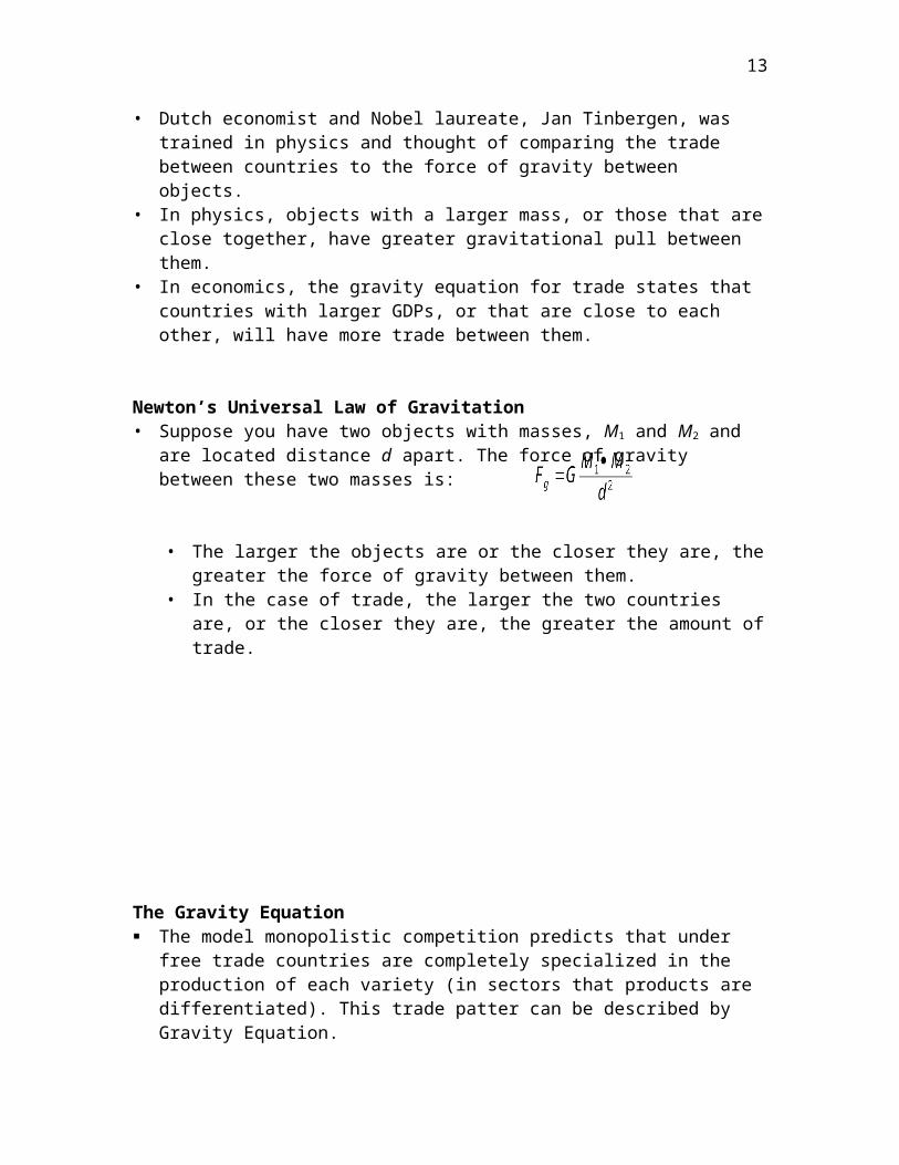
The Gravity Equation• Dutch economist and Nobel laureate, Jan Tinbergen, was trained in physics and
thought of comparing the trade between countries to the force of gravity between objects.
• In physics, objects with a larger mass, or those that are close together, have greater gravitational pull between them.
• In economics, the gravity equation for trade states that countries with larger GDPs, or that are close to each other, will have more trade between them.
Newton’s Universal Law of Gravitation
• Suppose you have two objects with masses, M1 and M2 and are located distance d apart. The force of gravity between these two masses is:
• The larger the objects are or the closer they are, the greater the force of gravity between them.
• In the case of trade, the larger the two countries are, or the closer they are, the greater the amount of trade.
9

The Gravity Equation The model monopolistic competition predicts that under free trade countries are
completely specialized in the production of each variety (in sectors that products are differentiated). This trade patter can be described by Gravity Equation.
Assuming that countries are specialized in different goods, the Gravity Equation states that the bilateral trade between two countries is directly proportional to the product of the countries GDP’s. Thus:
• Larger countries will tend to trade more with each other, • Countries that are more similar in their relative sizes will also trade more.
The constant term can also be interpreted as summarizing the effects of all factors, other than distance and size, that influence the amount of trade between two countries.
You can see from the equation that the larger the two countries are or the closer they are, the greater the amount of trade.
This is an implication of the monopolistic competition model we studied in this chapter.
Larger countries export more because they produce more product varieties, and import more because their demand is higher.
Deriving the gravity equation
• The demand for Country 1’s goods depends on:• The relative size of the importing country• The distance between the two countries• To measure the relative size of a country, we use its share of world GDP:
Share2 = GDP2/GDPW
A larger home market will attract disproportionately more firms (and hence more variety) and therefore becomes a net exporter. This is called the “home market effect”.
• With two countries trading, the larger market will produce a greater number of products and will be a net exporter of the differentiated good
• People in larger countries have larger income thus can afford larger variety of goods. That is why more variety is produced there (have assumed no transportation cost.
10
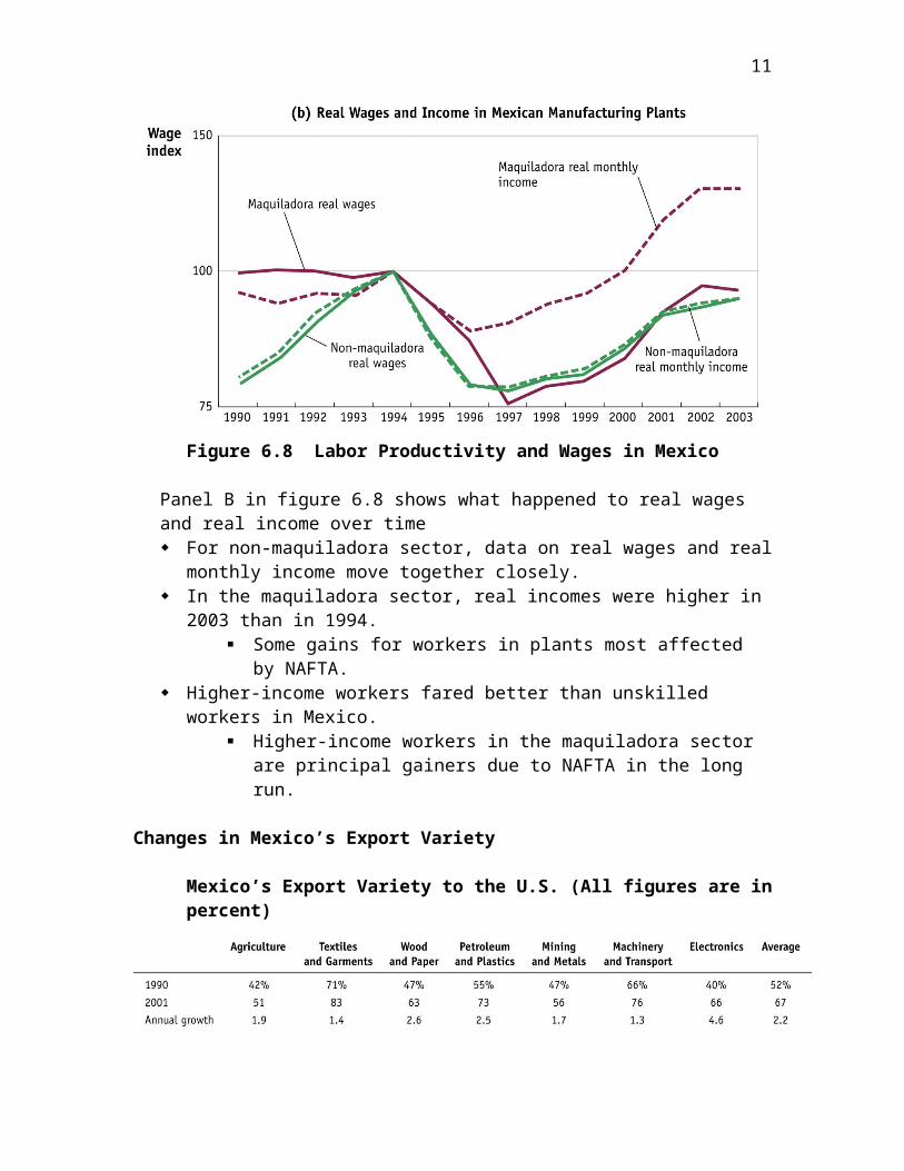
Figure 6.9 Gravity Equation for the United States and Canada, 1993
Gravity Equation for the United States and Canada, 1993 Plotted in these figures are the dollar value of exports in 1993 and the gravity term (plotted in log scale). Panel (a) shows these variables for trade between 10 Canadian provinces and 30 U.S. states. When the gravity term is 1, for example, the amount of trade between a province and state is $93 million.
Gravity Equation for the United States and Canada, 1993Panel (b) shows these variables for trade between 10 Canadian provinces. When the gravity term is 1, the amount of trade between the provinces is $1.3 billion, 14 times larger than between a province and a state.
11

These graphs illustrate two important points: there is a positive relationship between country size (as measured by GDP) and trade volume, and there is much more trade within Canada than between Canada and the United States.
If trade across borders happens to be less than trade within countries, there must be barriers to trade between those countries. Factors that make it easier or more difficult to trade goods between countries are often called border effects, and they include the following: Taxes imposed when imported goods enter into a country, tariffs Limits on the number of items allowed to cross the border, quotas Other administrative rules and regulations affecting trade, including the time required
for goods to clear customs Geographic factors such as whether the countries share a border Cultural factors such as whether the countries have a common language that might
make trade easier
The Gravity Equation and the Economies of Scale Gravity equation performs extremely well empirically for the industrialized countries
(and not well at all for non-OECD countries) This suggests that industrialized countries are specialized in different products, for
whatever reason. Davis and Weinsten (1996, 1999) using OECD data finds that
• The impact of local demand on production exceeds unity in a majority of industries.
• In particular they find that having a 10% greater demand for production will lead to 16% additional production in that country, meaning that net exports will rise.
This lends support to the idea that monopolistic competition explains national product specialization.
12
The Theory of External Economies Economies of scale can be either:
• Internal – The cost per unit depends on the size of an individual firm but not
necessarily on that of the industry.– The market structure will be imperfectly competitive with large
firms having a cost advantage over small (as of Kurgman Model)• External
– The cost per unit depends on the size of the industry but not necessarily on the size of any one firm.
– An industry will typically consist of many small firms and be perfectly competitive.
• Both types of scale economies are important causes of international trade.
Why a cluster of firms may be more efficient than an individual firm in isolation1- Specialized Suppliers
• In many industries, the production of goods and services and the development of new products require the use of specialized equipment or support services.
• An individual company does not provide a large enough market for these services to keep the suppliers in business.
A localized industrial cluster can solve this problem by bringing together many firms that provide a large enough market to support specialized suppliers.
This phenomenon has been extensively documented in the semiconductor industry located in Silicon Valley.
2- Labor Market Pooling• A cluster of firms can create a pooled market for workers with highly
specialized skills.• It is an advantage for:
Producers: They are less likely to suffer from labor shortages. Workers: They are less likely to become unemployed.
3- Knowledge Spillovers• Knowledge is one of the important input factors in highly innovative
industries.• The specialized knowledge that is crucial to success in innovative
industries comes from: Research and development efforts Reverse engineering Informal exchange of information and ideas
13

External Economies and Increasing Returns• External economies can give rise to increasing returns to scale at the level
of the national industry.• Forward-falling supply curve
The larger the industry’s output, the lower the price at which firms are willing to sell their output.
External Economies and Patterns of Trade• A country that has large production in some industry will tend to have low
costs of producing that good.• Countries that start out as large producers in certain industries tend to
remain large producers even if some other country could potentially produce the goods more cheaply.
Figure 6-9, below, illustrates a case where a pattern of specialization established by historical accident is persistent.
Copyright © 2003 Pearson Education, Inc. Slide 6-54
Figure 6-9: External Economies and Specialization
External Economies and International Trade
ACSWISS
Q1
P1
Price, cost (per watch)
Quantity of watchesproduced and demanded
ACTHAI2
1C0
D
14
S1= MCi , for i = to n
S2= MCi for i = to n’ >n
ACLR (Industry)
Q
D1D2
P

Trade and Welfare with External Economies• Trade based on external economies has more ambiguous effects on
national welfare than either trade based on comparative advantage or trade based on economies of scale at the level of the firm.
– An example of how a country can actually be worse off with trade than without is shown in Figure 6-10.
Copyright © 2003 Pearson Education, Inc. Slide 6-56
Figure 6-10: External Economies and Losses from Trade
External Economies and International Trade
ACSWISSP1
Price, cost (per watch)
Quantity of watchesproduced and demanded
ACTHAI2
1C0
DTHAIDWORLD
P2
Dynamic Increasing Returns• Learning curve
– It relates unit cost to cumulative output.– It is downward sloping because of the effect of the experience
gained though production on costs.
• Dynamic increasing returns– A case when costs fall with cumulative production over time,
rather than with the current rate of production.–
• Dynamic scale economies justify protectionism.– Temporary protection of industries enables them to gain
experience (infant industry argument)
15

Copyright © 2003 Pearson Education, Inc. Slide 6-58
Figure 6-11: The Learning Curve
External Economies and International Trade
L
Unit cost
Cumulativeoutput
L*
C*0
C1
QL
Summary In general, trade may be divided into two kinds:
Two-way trade in differentiated products within an industry (intraindustry trade).
Trade in which the products of one industry are exchanged for products of another (interindustry trade).
Trade can result from increasing returns or economies of scale, that is, from a tendency of unit costs to be lower at larger levels of output.
The presence of scale economies leads to a breakdown of perfect competition. Trade in under IRS must be analyzed using models of imperfect competition. In monopolistic competition, an industry contains a number of firms producing
differentiated products. Intraindustry trade benefits consumers through greater product variety and lower
prices.
Economies of scale can be internal or external. Dumping occurs when a firm charges a lower price abroad than it charges
domestically. Dumping can occur only if two conditions are met:
The industry must be imperfectly competitive. Markets must be geographically segmented.
External economies give an important role to history and accident in determining the pattern of international trade.
When external economies are important, countries can conceivably lose from trade.
16