Chapter 6: The Laplace Transform - National Chiao Tung...
54
Chapter 6: The Laplace Transform Chih-Wei Liu
Transcript of Chapter 6: The Laplace Transform - National Chiao Tung...
Chapter 6: The Laplace Transform
Chih-Wei Liu

Outline Introduction The Laplace Transform The Unilateral Laplace Transform Properties of the Unilateral Laplace Transform Inversion of the Unilateral Laplace Transform Solving Differential Equations with Initial Conditions Laplace Transform Methods in Circuit Analysis Properties of the Bilateral Laplace Transform Properties of the Region of convergence Inversion of the bilateral Laplace Transform
2

Outline The Transfer Function Causality and Stability Determining Frequency Response from Poles & Zeros
3

Introduction
4
The Laplace transform (LT) provides a broader characterization of continuous-time LTI systems and their interaction with signals than is possible with Fourier transform
Signal that is not absolutely integral
Two varieties of LT: Unilateral or one-sided Bilateral or two-sided The unilateral Laplace transform (ULT) is for solving differential
equations with initial conditions. The bilateral Laplace transform (BLT) offers insight into the nature of
system characteristics such as stability, causality, and frequency response.
Laplace transform
Fourier transform
A General Complex Exponential est
5
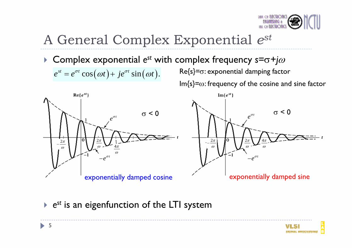
Complex exponential est with complex frequency s=+j
est is an eigenfunction of the LTI system
cos sin .st t te e t je t
te
tete
te
2
2
2
2
44
exponentially damped cosine exponentially damped sine
< 0 < 0
Re{s}=: exponential damping factor
Im{s}=: frequency of the cosine and sine factor

Eigenfunction Property of est
6
Transfer function
H(s) is the eigenvalue of the eigenfunction est
Polar form of H(s):
LTI system, h(t)x(t) = est y(t) = x(t) h(t)
)(
)(
)(
)()()()()(
)(
sHe
dehe
deh
dtxhtxthty
st
sst
ts
sH s h e d
( ) j sH s H s e
H(s) amplitude of H(s); (s) phase of H(s)
cos sin
j t jt
t t
y t H j e e
H j e t j j H j e t j
Then j s sty t H s e e Let s = + j
The LTI system changes the amplitude of the input by H( + j ) and shifts the phase of the sinusoidal components by ( + j ).

The Laplace Transform
7
Definition: The Laplace transform of x(t): Definition: The inverse Laplace transform of X(s):
A representation of arbitrary signals as a weighted superposition of eigenfunctions est with s=+j. We obtain
Hence
stX s x t e dt
12
j st
jx t X s e ds
j
x t X sL
j t
t j t
H j h t e dt
h t e e dt
)()( jHeth FTt
12
t j th t e H j e d
j
st
tj
dsesHj
dejHth
)(21
)(21)( )(
s = + jds = jd
Laplace transform is the FT of h(t)e t

Convergence of Laplace Transform
8
LT is the FT of x(t)e t A necessary condition for convergence of the LT is the absolute integrability of x(t)e t:
The range of for which the Laplace transform converges is termed the region of convergence (ROC).
Convergence example:
tx t e dt
1. Fourier transform of x(t)=e tu(t) does not exist, since x(t) is not absolutely integrable.
2. But x(t)et =e(1)tu(t) is absolutely integrable, if >1, i.e. ROC, so the Laplace transform of x(t), which is the Fourier transform of x(t)et, does exist.
et x(t) et

j
The s-Plane, Poles, and Zeros
9
To represent s graphically in terms of complex plane
s = + j Horizontal axis of s-plane = real part of s; vertical axis of s-plane = imaginary part of s.
Relation between FT and LT:
The j-axis divides the s-plane in half: left-half and right-half s-plane Laplace transform X(s):
0
X j X s
the Fourier transform is given by the LT evaluated along the imaginary axis
pole; zero
1
1 01
1 1 0
M MM M
N NN
b s b s bX ss a s a s a
1
1
MM kk
Nkk
b s cX s
s d
ck = zeros of X(s); dk = poles of X(s)
j
Example 6.1
10
<Sol.>
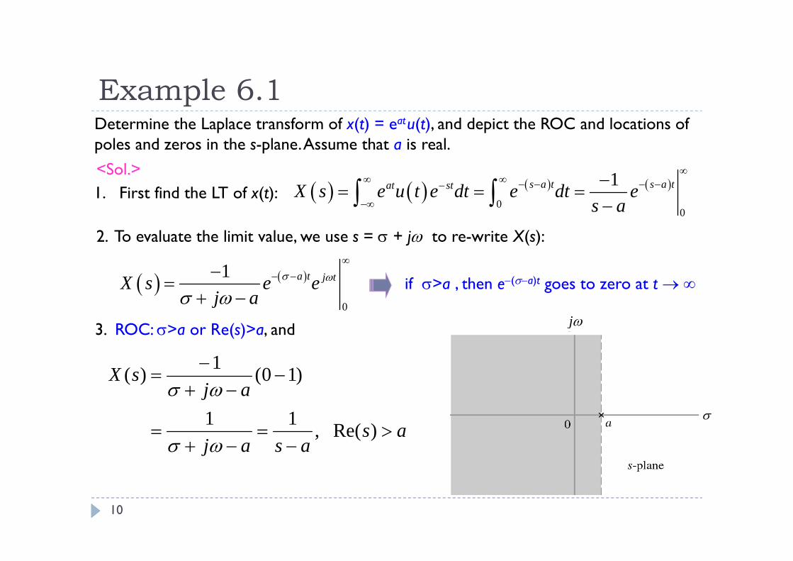
Determine the Laplace transform of x(t) = eatu(t), and depict the ROC and locations of poles and zeros in the s-plane. Assume that a is real.
1. First find the LT of x(t): 0
0
1s a t s a tat stX s e u t e dt e dt es a
2. To evaluate the limit value, we use s = + j to re-write X(s):
0
1 a t j tX s e ej a
3. ROC: >a or Re(s)>a, and
if >a , then e(a)t goes to zero at t
asasaj
ajsX
)Re( ,11
)10(1)(
j
Example 6.2
11
<Sol.>
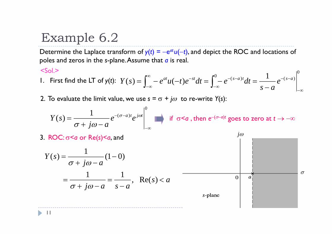
Determine the Laplace transform of y(t) = eatu(t), and depict the ROC and locations of poles and zeros in the s-plane. Assume that a is real.
1. First find the LT of y(t):
2. To evaluate the limit value, we use s = + j to re-write Y(s):
3. ROC: <a or Re(s)<a, and
if <a , then e(a)t goes to zero at t
asasaj
ajsY
)Re( ,11
)01(1)(
0)(0 )( 1)()(
astasstat e
asdtedtetuesY
0)(1)(
tjta ee
ajsY

Concluding Remarks
12
Examples 6.1 & 6.2 reveal that the same Laplace transform but different ROCs for the different signals x(t) and y(t)
This ambiguity occurs in general with signals that are one sided. To see why, let x(t)=g(t)u(t) and y(t)= g(t)u( t). We may thus write
The value of s for which the integral represented by G(s, ) converges differ from those for which the integral represented by G(s, ) converges, and thus the ROCs are different
0
, ,0
stX s g t e dt
G s G s
where , stG s t g t e dt
And, 0
0, ,0st stY s g t e dt g t e dt G s G s
We conclude that X(s) = Y(s) whenever G(s, ) = G(s, ).
The ROC must be specified for the Laplace transform to be unique !!!
Outline Introduction The Laplace Transform The Unilateral Laplace Transform Properties of the Unilateral Laplace Transform Inversion of the Unilateral Laplace Transform Solving Differential Equations with Initial Conditions Laplace Transform Methods in Circuit Analysis Properties of the Bilateral Laplace Transform Properties of the Region of convergence Inversion of the bilateral Laplace Transform
13

The Unilateral (or One-Sided) LT
14
We may assume that the signals involved are causal, that is, zero for t < 0.
The unilateral Laplace transform (ULT) of a signal x(t) is defined by
Note that ULT and LT are equivalent for signals that are causal.
The ambiguity of LT is removed in ULT
0
stX s x t e dt
The lower limit of 0 implies that we do include discontinuities and impulses
ux t X sL
astue ULTat
1)(
Since one-sided, do not specify ROC
asas
tue LTat
}Re{ ROC with1)(equivalent to
Properties of ULT
15
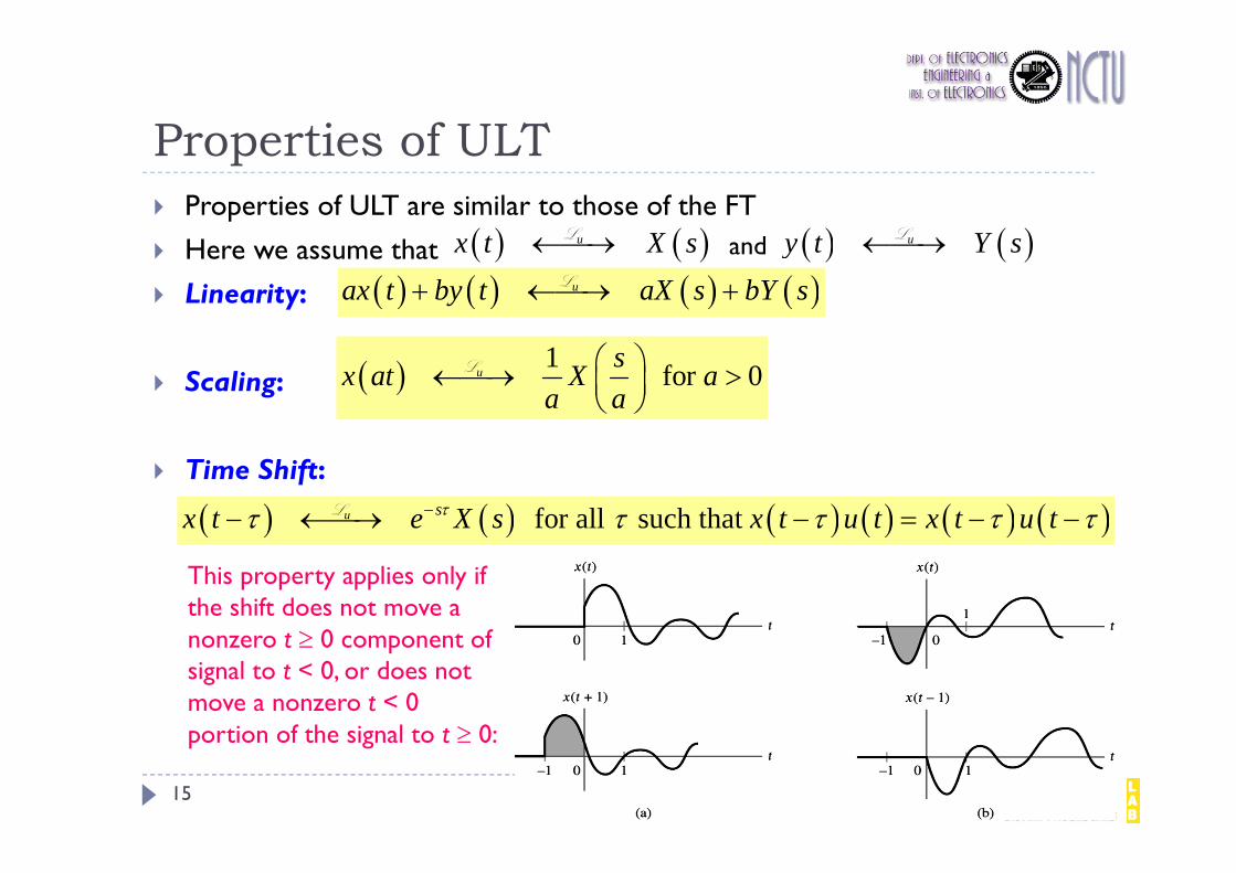
Properties of ULT are similar to those of the FT
Here we assume that
Linearity:
Scaling:
Time Shift:
ux t X sL and uy t Y sL
uax t by t aX s bY s L
1 for 0usx at X a
a a
L
for all such that u sx t e X s x t u t x t u t L
This property applies only if the shift does not move a nonzero t 0 component of signal to t < 0, or does not move a nonzero t < 0 portion of the signal to t 0:

Properties of ULT
16
s-Domain Shift:
Convolution:
Differentiation in the s-Domain:
Example 6.3:
00
us te x t X s s L
* ux t y t X s Y sL
udtx t X sds
L
Find the unilateral Laplace transform of 3 *tx t e u t tu t <Sol.>Since 3 1
3ute u t
s
L and 1uu t
sL
Apply the s-domain differentiation property, we have 21/utu t sL
Now, from the convolution property, we obtain
3
2
1*3
utx t e u t tu t X ss s
L
2)3(1)(
sssX
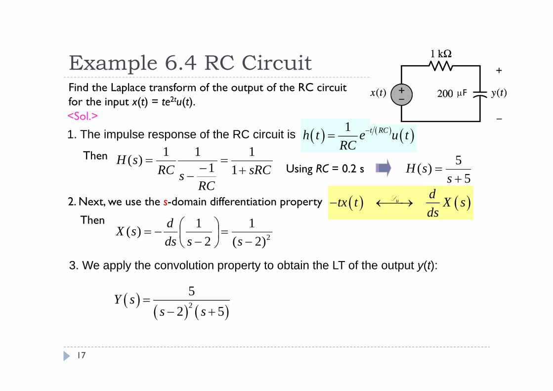
1 t RCh t e u tRC
Example 6.4 RC Circuit
17
Find the Laplace transform of the output of the RC circuit for the input x(t) = te2tu(t). <Sol.>
1. The impulse response of the RC circuit is
ThensRC
RCsRC
sH
11
111)(
Using RC = 0.2 s5
5)(
s
sH
2. Next, we use the s-domain differentiation property
F
udtx t X sds
L
2)2(1
21)(
ssdsdsX
Then
3. We apply the convolution property to obtain the LT of the output y(t):
2
52 5
Y ss s

Properties of ULT
18
Differentiation in the Time-Domain:
0 0
u st std x t x t e s x t e dtdt
L 0
u std dx t x t e dtdt dt
L
=
Integration by part
0ud x t sX s xdt
L x(t)e-st approaches zero as t
1 2
1 20 0
12 1
10
0
n nn
n nt t
nn n
nt
d ds X s x t s x tdt dt
ds x t s xdt
u
n
n
d x tdt
L
The general form for the differentiation property

Properties of ULT
19
Integration Property:
Initial- and Final-Value Theorem:
1 0
ut x X s
x ds s
L
where 01 0x x d
is the area under x(t) from t = to t = 0.
lim 0s
sX s x
0lims
sX s x
)0()()(0
xssXdtetxdtd stRecall Then
)0()()()()(lim)0()(lim00000
xxtdxdttxdtddtetx
dtdxssX st
ss
0
lims
sX s x
(1)
0)(lim)0()(lim0
dtetx
dtdxssX st
ss(2) )0()(lim
xssX
s

Remarks
20
For initial-value theorem:
This theorem does not apply to rational functions X(s) in which the order of the numerator polynomial is greater than or equal to that of the denominator polynomial
For final-value theorem
This theorem applies only if all the poles of X(s) are in the left half of the s-plane, with at most a single pole at s=0
Example 6.6
<Sol.>Determine the initial and final values of a signal x(t) whose ULT is
7 102
sX ss s
1. Initial value:
7 10 7 100 lim lim 7
2 2s s
s sx ss s s
2. Final value:
0 0
7 10 7 10lim lim 52 2s s
s sx ss s s
Note that X(s) is the Laplace transform of 2( ) 5 ( ) 2 ( )tx t u t e u t
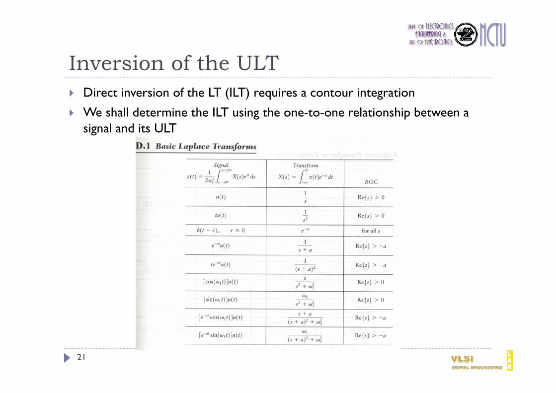
Inversion of the ULT
21
Direct inversion of the LT (ILT) requires a contour integration
We shall determine the ILT using the one-to-one relationship between a signal and its ULT

Inversion by Partial-Fraction Expansion
22
The inverse transform can be obtained by expressing X(s) as a sum of terms for which we already known the time function
Suppose
B sX s
A s
11 1 0
11 1 0
M MM M
N NN
b s b s b s bs a s a s a
M < N
If M N, we may use long division to express X(s) as 0
M Nk
kk
X s c s X s
1. Using the differentiation property and the pair 1ut L
We obtain 0 0
u
M N M Nk k
k kk k
c t c s
L
2. Factor the denominator polynomial as a product of pole factors to obtain
B sX s
A s
11 1 0
1
p pp p
Nkk
b s b s b s b
s d
P < N

Inversion by Partial-Fraction Expansion
23
Case I: If all poles dk are distinct:
Case II: If a pole di is repeated r times:
1
Nk
k k
AX ss d
k ud t k
kk
AA e u ts d
L
B sX s
A s
11 1 0
1
p pp p
Nkk
b s b s b s b
s d
1 2
2, , , ri i ir
i i i
A A As d s d s d
Apply differentiation in the s-domain:
1
1 !k u
nd t
nk
At Ae u tn s d
L

Example 6.7
24
<Sol.>
Find the inverse Laplace transform of 2
3 41 2sX s
s s
Use a partial-fraction expansion of X(s) to write
31 221 2 2
AA AX ss s s
Solving for A1, A2, and A3, we obtain 2
1 1 21 2 2
X ss s s
1) The pole of the first term is at s=-1, so
11
ute u ts
L
2) The second term has pole at s = -2; thus,
2 12
ute u ts
L
3) The double pole in the last term is also at s = -2; hence,
22
222
utte u ts
L 2 22t t tx t e u t e u t te u t
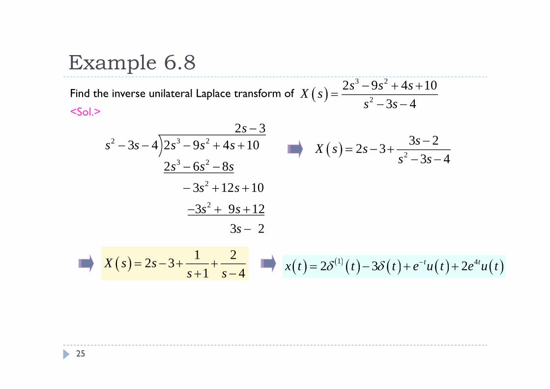
Example 6.8
25
<Sol.>
Find the inverse unilateral Laplace transform of 3 2
2
2 9 4 103 4
s s sX ss s
2 3 2
3 2
2
2
2 33 4 2 9 4 10
2 6 8 3 12 10 3 9 12 3 2
ss s s s s
s s ss ss s
s
2
3 22 33 4
sX s ss s
1 22 31 4
X s ss s
1 42 3 2t tx t t t e u t e u t

Conjugate Poles
26
If the coefficients in the denominator are real, then all the complex poles occur in complex-conjugate pairs.
Combine complex-conjugate poles to obtain real-valued expansion coefficients
1. Suppose that + j0 and j0 make up a pair of complex-conjugate poles. Then
1 2
0 0
A As j s j
A1 and A2 must be complex conjugates of each other it’s hard to solve A1 and A2 from real-valued coefficients
2. Combine conjugate poles: + j0 and j0. Then
1 2 1 2
2 20 0 0
B s B B s Bs j s j s
where both B1 and B2 are real valued.
1 2 01 2
2 2 22 2 20 0 0
C s CB s Bs s s
where C1=B1 and C2=(B2 + α)/ω0
20
21
01 )()()()cos(
s
sCtuteC ULTt20
202
02 )()()sin(
sCtuteC ULTt
in term of the perfect square

Example 6.9
27
Find the inverse Laplace transform of
<Sol.>
2
3 2
4 62
sX ss s
1 221 1 1
B s BAX ss s
)1)1)((1()22)(1(2 2223 ssssssswrite the quadratic s2 + 2s + 2 in terms of the perfect square
Then
2
211
4 61 21 1s
s
sA X s ss
221 2
21 1 2 2
4 6 2 1 1 1
2 4 4
s s B s B s
B s B B s B
2
2 2
2 2 21 1 1
2 1 12 41 1 1 1 1
sX ss s
ss s s
2 2 cos 4 sint t tx t e u t e t u t e t u t

Outline Introduction The Laplace Transform The Unilateral Laplace Transform Properties of the Unilateral Laplace Transform Inversion of the Unilateral Laplace Transform Solving Differential Equations with Initial Conditions Laplace Transform Methods in Circuit Analysis Properties of the Bilateral Laplace Transform Properties of the Region of convergence Inversion of the bilateral Laplace Transform
28

Example 6.6: Solving Differential Equations with Initial Conditions
29
Recall 0ud x t sX s xdt
L
The initial condition
<Sol.>
Use the Laplace transform to find the voltage across the capacitor, y(t), for the RC circuit in response to the applied voltage x(t) = (3/5)e-2tu(t) and initial condition y(0-)=-2. F
Using Kirchhoff’s voltage law, we have the differential equation
1 1d y t y t x tdt RC RC
RC = 0.2 s 5 5d y t y t x t
dt
0 5 5sY s y Y s X s 1 5 05
Y s X s ys
3/ 5( ) ( )
2ux t X s
s
L y(0-)=-2
3 22 5 5
Y ss s s
1 1 2 1 32 5 5 2 5
Y ss s s s s
2 53t ty t e u t e u t
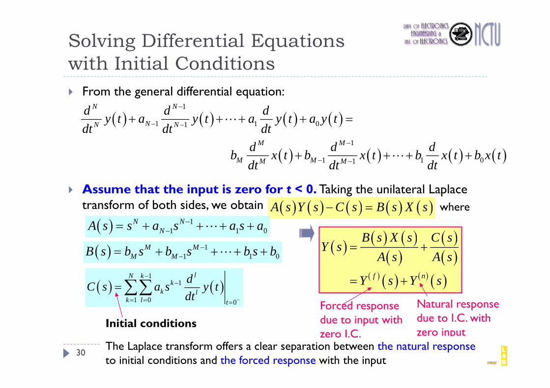
Solving Differential Equations with Initial Conditions
30
From the general differential equation:
Assume that the input is zero for t < 0. Taking the unilateral Laplace transform of both sides, we obtain
1
1 1 01
1
1 1 01
N N
NN N
M M
M MM M
d d dy t a y t a y t a y tdt dt dt
d d db x t b x t b x t b x tdt dt dt
A s Y s C s B s X s 1
1 1 0N N
NA s s a s a s a
11 1 0
M MM MB s b s b s b s b
1
1
1 0 0
lN kk
k lk l t
dC s a s y tdt
where
f n
B s X s C sY s
A s A s
Y s Y s
Natural response due to I.C. with zero input
Initial conditions
The Laplace transform offers a clear separation between the natural response to initial conditions and the forced response with the input
Forced response due to input with zero I.C.

Example 6.11
31
<Sol.>
Use the unilateral Laplace transform to determine the output of the system described by the differential equation
2
2 5 6 6d d dy t y t y t x t x tdt dt dt
in response to the input x(t) = u(t).
0 1y and 0
2t
d y tdt
Identity the forced response of the system, y(f)(t), and the natural response y(n)(t).
1. Apply ULT on the both sides of the differential equations, we obtain:
2
0
5 6 0 5 0 6t
ds s Y s y t sy y s X sdt
Assume that
0
2 2
0 5 065 6 5 6
t
dsy y t ys X s dtY ss s s s
)()()( )()( sYsYsY nf
6
2 3f sY s
s s s
7
2 3n sY s
s s
and
2 32f t ty t u t e u t e u t 2 35 4n t ty t e u t e u t
Outline Introduction The Laplace Transform The Unilateral Laplace Transform Properties of the Unilateral Laplace Transform Inversion of the Unilateral Laplace Transform Solving Differential Equations with Initial Conditions Laplace Transform Methods in Circuit Analysis Properties of the Bilateral Laplace Transform Properties of the Region of convergence Inversion of the bilateral Laplace Transform
32

Bilateral Laplace Transform (BLT)
33
The BLT involves the values of the signal for both t 0 and t < 0
Assume that
Linearity:
Example 6.14
stx t X s x t e dt
L BLT is well suited problems involving
noncausal signals and systems
( ) ( ) with ROC xx t X s RL
( ) ( ) with ROC yy t Y s RL ROC should be given
( ) ( ) ( ) ( ) with ROC x yax t by t aX s bY s R R L
The ROC may be larger than Rx Ry if a pole and a zero cancel in aX(s) + bY(s).
2 12
tx t e u t X ss
L with ROC Re 2s and
2 3 1
2 3t ty t e u t e u t Y s
s s
L with ROC Re 2s
31
)3)(2(1)3()()(
sss
ssYsXThen
3)Re( ROC with)()()( 3 stuetytx t
If the intersection of ROCs is an empty set, the LT of ax(t)+by(t) does not exist

Properties of BLT
34
Time Shift:
Differentiation in the Time Domain:
Integration with respect to Time:
stx t e X s LSince the BLT is evaluated over both positive and negative t, the ROC is unchanged by a time shift.
d x t sX sdt
L with ROC at least Rx
The ROC associated with sX(s) may be larger than Rx if X(s) has a single pole at s = 0 on the ROC boundary
t X sx d
s
L with ROC Re 0xR s
Integration corresponds to division by s. Since this introduces a pole at s = 0 and we are integrating to the right, the ROC must lie to the right of s = 0

Example 6.15
35
<Sol.>Find the Laplace transform of
23 2
2 2tdx t e u tdt
1. We know from Ex. 6.1 that 3 13
te u ts
L with ROC Re 3s
2. The time-shift property implies that
3 2 2123
t se u t es
L with ROC Re 3s
3. Apply the time-differentiation property twice, we obtain
with ROC Re 3s 2 2
3 2 22 2
3t sd sx t e u t X s e
dt s
L

Properties of the ROC
36
Recall that the BLT is not unique unless the ROC is specified.
The ROC is related to he characteristics of a signal x(t) indeed.
(1) For rational LTs, the ROC cannot contain any polesSuppose d is a pole of X(s), then X(d)=
(2) The ROC consists of strips parallel to the j-axis in the s-plane.
(3) The ROC for a finite-duration and bounded x(t) is the entire s-plane
Convergence of the BLT for a signal x(t) implies that
tI x t e dt
for some values of .
The set of with finite I() determines the ROC of BLT.
ROC consists of strips parallel to the j-axis in the s-plane.
, 0
, 0
b t
a
bt
a
I Ae dt
A e
A b a
I() is finite for all finite values of

Properties of the ROC
37
(4) Convergence of the BLT for a signal x(t) implies that
tI x t e dt
for some values of .
Let’s separate I() into two one-sided parts, i.e. positive- and negative-time sections:
I I I
where 0 tI x t e dt
0
tI x t e dt
and
In order for I() to be finite, both I() and I() must be finite.
This implies that x(t) must be bounded in some sense.
Suppose we can bound x(t) for both I() and I() by finding the smallest p s.t.
, 0ptx t Ae t and largest n s.t. , 0ntx t Ae t
A signal x(t) that satisfies these bounds is said to be of exponential order.
x(t) grows no faster than ept for positive t and ent for negative t
Properties of the ROC
38
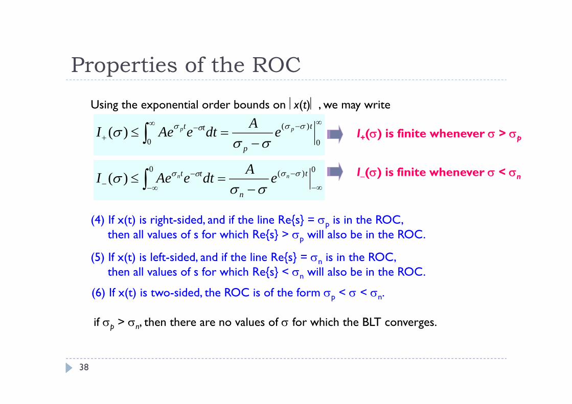
Using the exponential order bounds on x(t) , we may write
I+() is finite whenever > p
0)(0)(
t
n
tt nn eAdteAeI
0
)(
0)( t
p
tt pp eAdteAeI
I() is finite whenever < n
(4) If x(t) is right-sided, and if the line Re{s} = p is in the ROC, then all values of s for which Re{s} > p will also be in the ROC.
(5) If x(t) is left-sided, and if the line Re{s} = n is in the ROC, then all values of s for which Re{s} < n will also be in the ROC.
(6) If x(t) is two-sided, the ROC is of the form p < < n.
if p > n, then there are no values of for which the BLT converges.
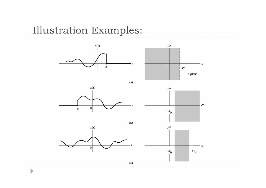
Illustration Examples:
p n
p
j
j
j
n
p
np

Example 6.16
40
Consider the two signals 21
t tx t e u t e u t 22
t tx t e u t e u t and
Identify the ROC associated with the bilateral Laplace transform of each signal.
<Sol.>
1. We check the absolute integrability of x1(t) e t by writing
1 1
0 1 2
0
01 2
0
1 11 2
t
t t
t t
I x t e dt
e dt e dt
e e
The first converges for < 1, while the second term converges for > 2. Hence, both terms converge for 2 < < 1. This is the intersection of the ROC for each term.
The ROC for each term and the intersection of the ROCs, which is shown as the doubly shaded region, are depicted in Fig. 6.15 (a).
41
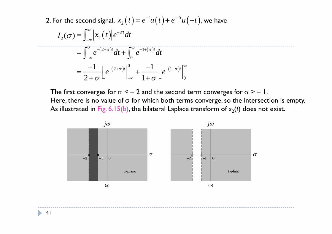
2. For the second signal, , we have
1 2
0 2 1
0
02 1
0
1 12 1
t
t t
t t
I x t e dt
e dt e dt
e e
)(2 I
22
t tx t e u t e u t
The first converges for < 2 and the second term converges for > 1. Here, there is no value of for which both terms converge, so the intersection is empty. As illustrated in Fig. 6.15(b), the bilateral Laplace transform of x2(t) does not exist.
jj
Inversion of the BLT
42
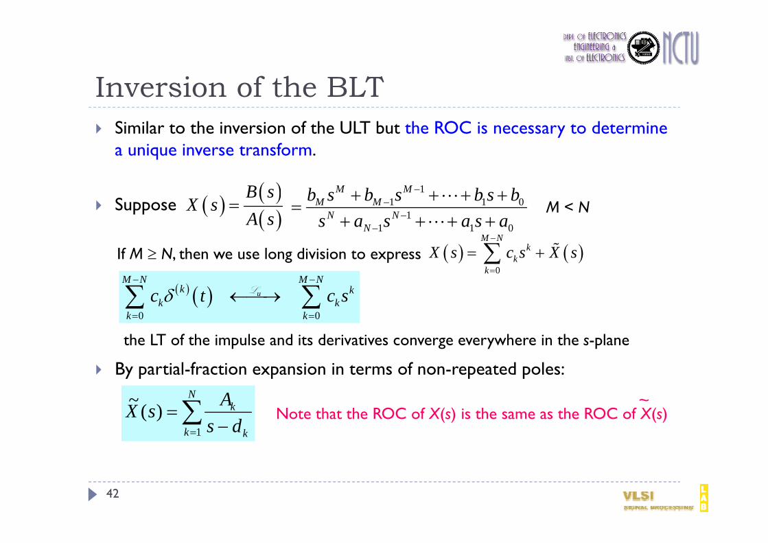
Similar to the inversion of the ULT but the ROC is necessary to determine a unique inverse transform.
Suppose
By partial-fraction expansion in terms of non-repeated poles:
B sX s
A s
11 1 0
11 1 0
M MM M
N NN
b s b s b s bs a s a s a
If M N, then we use long division to express 0
M Nk
kk
X s c s X s
M < N
0 0
u
M N M Nk k
k kk k
c t c s
L
Note that the ROC of X(s) is the same as the ROC of X(s)~
the LT of the impulse and its derivatives converge everywhere in the s-plane
N
k k
k
dsAsX
1
)(~

Inversion of BLT
43
Two possibilities for the inverse BLT of X(s) 1. Right-sided
2. Left-sided
Example 6.17
~
with ROC Re( )kd t kk k
k
AA e u t s ds d
L
with ROC Re( )kd t kk k
k
AA e u t s ds d
L
The ROC of a right-side exponential signal lies to the right of the pole, while the ROC of a left-sided exponential signal lies to the left of the pole.
Find the inverse bilateral Laplace transform of 5 7
1 1 2sX s
s s s
with ROC 1 Re 1s
<Sol.>Use the partial-fraction expansion 1 2 1
1 1 2X s
s s s
j
right-sided left-sided
22t t tx t e u t e u t e u t
Inversion of BLT
44
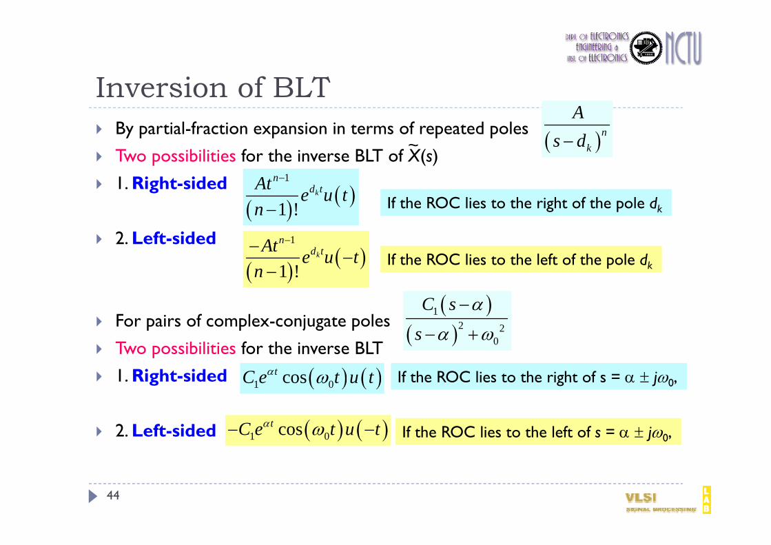
By partial-fraction expansion in terms of repeated poles
Two possibilities for the inverse BLT of X(s) 1. Right-sided
2. Left-sided
For pairs of complex-conjugate poles
Two possibilities for the inverse BLT
1. Right-sided
2. Left-sided
nk
As d~
1
1 !k
nd tAt e u t
n
1
1 !k
nd tAt e u t
n
If the ROC lies to the left of the pole dk
If the ROC lies to the right of the pole dk
12 2
0
C ss
1 0costC e t u t If the ROC lies to the right of s = j0,
1 0costC e t u t If the ROC lies to the left of s = j0,
Some Remarks
45
Causality If the signal is known to be causal, then we choose the right-sided
inverse transform of each term. (i.e. the unilateral Laplace transform)
Stability A stable signal is absolutely integrable and thus has a Fourier transform;
stability and the existence of Fourier transform (i.e. Re(s)=0) are equivalent conditions
In both cases, the ROC includes the jω-axis in the s-plane, or Re(s) = 0. The inverse LT of a stable signal is obtained by comparing the poles’
locations with jω-axis. If a pole lies to the left/right of the jω-axis, then the right/left-sided
inverse transform is chosen (the ROC should include the j-axis)
Outline The Transfer Function Causality and Stability Determining Frequency Response from Poles & Zeros
46

The Transfer Function
47
Recall that the transfer function H(s) of an LTI system is
If we take the bilateral Laplace transform of y(t), then
From differential equation:
sH s h e d
LTI system, h(t)x(t) y(t) = x(t) h(t)
x(t) = est y(t) = H(s)est
Y s H s X s
Y sH s
X s This definition applies only at
values of s for which X(s) 0
0 0
k kN M
k kk kk k
d da y t b x tdt dt
After Substituting est for x(t) and estH(s) for y(t), we obtain
0 0
k kN Mst st
k kk kk k
d da e H s b edt dt
rational transfer function
1
1
Mkk
Nkk
b s cH s
s d
0
0
M kkk
N kkk
b sH s
a s
Knowledge of the poles dk, zeros ck, and factor completely determine the system /M Nb b a
Causality and Stability
48
j
j
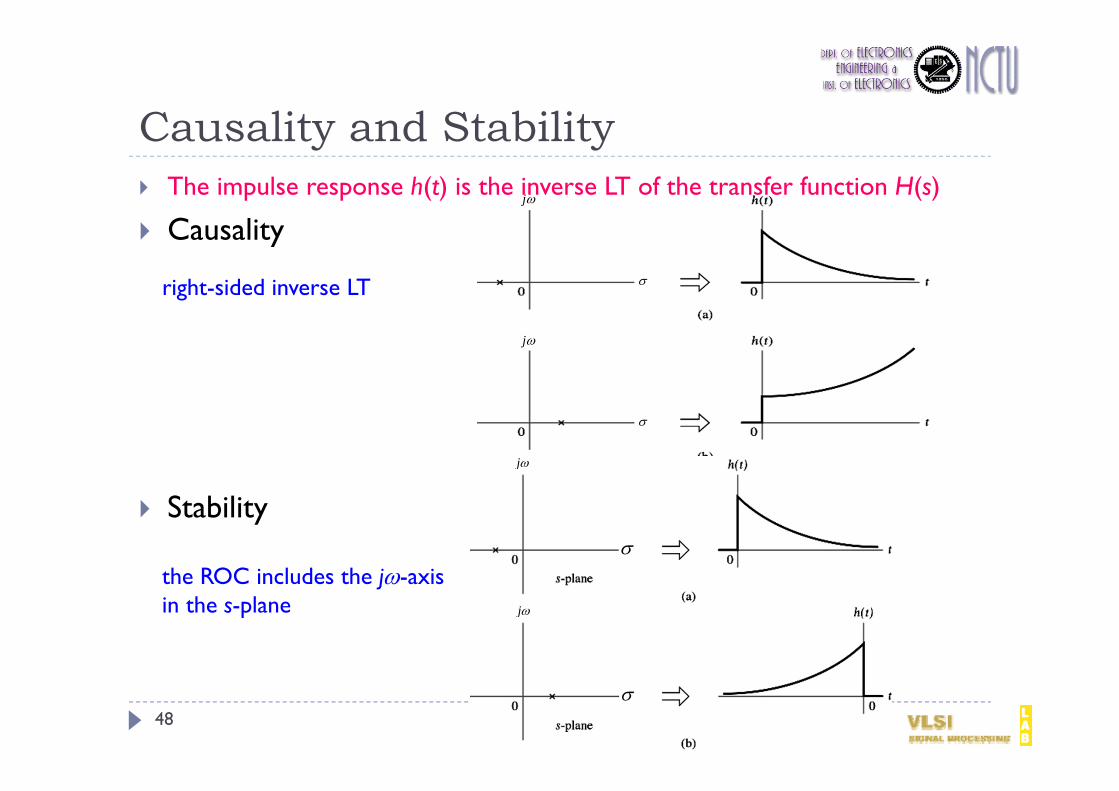
The impulse response h(t) is the inverse LT of the transfer function H(s)
Causality
Stability
j
j
right-sided inverse LT
the ROC includes the j-axis in the s-plane

Causal and Stable LTI System
49
To obtain a unique inverse transform of H(s), we must know the ROC or have other knowledge(s) of the impulse response
The relationships between the poles, zeros, and system characteristics can provide some additional knowledges
Systems that are stable and causal must have all their poles in the left half of the s-plane:
j

Example 6.21
50
<Sol.>
A system has the transfer function 2 13 2
H ss s
Find the impulse response, (a) assuming that the system is stable; (b) assuming that the system is causal; (c) can this system be both stable and causal?
(a) This system has poles at s = 3 and s = 2.
3 22 t th t e u t e u t Stable the ROC contains j-axis. the pole at s=3 contributes a right-sided term; the pole at s=2 contributes a left-sided term.
(b) This system has poles at s = 3 and s = 2.
Causal right-sided )()(2)( 23 tuetueth tt
(c) This system has poles at s = 3 and s = 2 this system cannot be both stable and causal

Inverse System
51
Given an LTI system with impulse response h(t), the impulse response of the inverse system, h inv(t), satisfies the condition *invh t h t t
1invH s H s 1invH s
H sor
a stable and causal inverse system exists only if all of the zeros of H(s) are in the left half of the s-plane.
the poles of the inverse system Hinv(s) are the zeros of H(s), and vice versa
A (stable and causal) H(s) has all of its poles and zeros in the left half of the s-plane
H(s) is minimum phase.
A nonminimum-phase system cannot have a stable and causal inverse system.

Example 6.22
52
<Sol.>
Consider an LTI system described by differential equation
2
23 2d d dy t y t x t x t x tdt dt dt
Find the transfer function of the inverse system. Is it a stable and causal inverse system?
First find the system’s transfer function H(s):
2 23
Y s s sH sX s s
2
1 3 32 1 2
inv s sH sH s s s s s
The inverse system has pole at s =1 and s =-2. Hinv(s) cannot be both stable and causal.

Determining Frequency Response from Poles & Zeros
53
Control system

Summary The Laplace transform represents continuous-time signals
as weighted superpositions of complex exponentials The transfer function is the Laplace transform of the impulse
response The unilatreal Laplace transform applies to causal signals (or one-
sided signals) The bilateral Laplace transform applies to two-sided signals;
it is not unique unless the ROC is specified.
The Laplace transform is most often used in the transient and stability analysis of system
The Fourier transform is usually employed as a signal representation tool and in solving
system problems in which steady-state characteristics are of interest.