Chapter 6 MIDI and Sound Synthesis - Juniata...
72
This material is based on work supported by the National Science Foundation under CCLI Grant DUE 0717743, Jennifer Burg PI, Jason Romney, Co-PI. 6 Chapter 6 MIDI and Sound Synthesis ................................................ 2 6.1 Concepts .................................................................................. 2 The Beginnings of Sound Synthesis ........................................ 2 6.1.1 MIDI Components ................................................................ 4 6.1.2 MIDI Data Compared to Digital Audio ..................................... 7 6.1.3 Channels, Tracks, and Patches in MIDI Sequencers ................ 11 6.1.4 A Closer Look at MIDI Messages .......................................... 14 6.1.5 Binary, Decimal, and Hexadecimal Numbers .................... 14 6.1.5.1 MIDI Messages, Types, and Formats ............................... 15 6.1.5.2 Synthesizers vs. Samplers .................................................. 17 6.1.6 Synthesis Methods ............................................................. 19 6.1.7 Synthesizer Components .................................................... 21 6.1.8 Presets ....................................................................... 21 6.1.8.1 Sound Generator .......................................................... 21 6.1.8.2 Filters ......................................................................... 22 6.1.8.3 Signal Amplifier ............................................................ 23 6.1.8.4 Modulation .................................................................. 24 6.1.8.5 LFO ............................................................................ 24 6.1.8.6 Envelopes.................................................................... 25 6.1.8.7 MIDI Modulation........................................................... 26 6.1.8.8 6.2 Applications ............................................................................ 27 Linking Controllers, Sequencers, and Synthesizers ................. 27 6.2.1 Creating Your Own Synthesizer Sounds ................................ 33 6.2.2 Making and Loading Your Own Samples ................................ 34 6.2.3 Data Flow and Performance Issues in Audio/MIDI Recording ... 38 6.2.4 Non-Musical Applications for MIDI ........................................ 39 6.2.5 MIDI Show Control ....................................................... 39 6.2.5.1 MIDI Relays and Footswitches ........................................ 41 6.2.5.2 MIDI Time Code ........................................................... 42 6.2.5.3 MIDI Machine Control ................................................... 45 6.2.5.4 6.3 Science, Mathematics, and Algorithms ....................................... 46 MIDI SMF Files .................................................................. 46 6.3.1 Shaping Synthesizer Parameters with Envelopes and LFOs ...... 48 6.3.2 Type of Synthesis .............................................................. 48 6.3.3 Table-Lookup Oscillators and Wavetable Synthesis ........... 48 6.3.3.1 Additive Synthesis ........................................................ 50 6.3.3.2 Subtractive Synthesis ................................................... 51 6.3.3.3 Amplitude Modulation (AM)............................................ 51 6.3.3.4 Ring Modulation ........................................................... 56 6.3.3.5 Phase Modulation (PM) .................................................. 57 6.3.3.6 Frequency Modulation (FM)............................................ 59 6.3.3.7 Creating A Block Synthesizer in Max ..................................... 60 6.3.4 6.4 References ............................................................................. 72
-
Upload
truongdieu -
Category
Documents
-
view
235 -
download
3
Transcript of Chapter 6 MIDI and Sound Synthesis - Juniata...

This material is based on work supported by the National Science Foundation under CCLI Grant DUE 0717743, Jennifer Burg PI, Jason Romney, Co-PI.
6 Chapter 6 MIDI and Sound Synthesis ................................................ 2
6.1 Concepts .................................................................................. 2
The Beginnings of Sound Synthesis ........................................ 2 6.1.1
MIDI Components ................................................................ 4 6.1.2 MIDI Data Compared to Digital Audio ..................................... 7 6.1.3
Channels, Tracks, and Patches in MIDI Sequencers ................ 11 6.1.4 A Closer Look at MIDI Messages .......................................... 14 6.1.5
Binary, Decimal, and Hexadecimal Numbers .................... 14 6.1.5.1 MIDI Messages, Types, and Formats ............................... 15 6.1.5.2
Synthesizers vs. Samplers .................................................. 17 6.1.6 Synthesis Methods ............................................................. 19 6.1.7
Synthesizer Components .................................................... 21 6.1.8 Presets ....................................................................... 21 6.1.8.1
Sound Generator .......................................................... 21 6.1.8.2 Filters ......................................................................... 22 6.1.8.3
Signal Amplifier ............................................................ 23 6.1.8.4
Modulation .................................................................. 24 6.1.8.5 LFO ............................................................................ 24 6.1.8.6
Envelopes .................................................................... 25 6.1.8.7 MIDI Modulation ........................................................... 26 6.1.8.8
6.2 Applications ............................................................................ 27
Linking Controllers, Sequencers, and Synthesizers ................. 27 6.2.1
Creating Your Own Synthesizer Sounds ................................ 33 6.2.2 Making and Loading Your Own Samples ................................ 34 6.2.3
Data Flow and Performance Issues in Audio/MIDI Recording ... 38 6.2.4 Non-Musical Applications for MIDI ........................................ 39 6.2.5
MIDI Show Control ....................................................... 39 6.2.5.1 MIDI Relays and Footswitches ........................................ 41 6.2.5.2
MIDI Time Code ........................................................... 42 6.2.5.3 MIDI Machine Control ................................................... 45 6.2.5.4
6.3 Science, Mathematics, and Algorithms ....................................... 46
MIDI SMF Files .................................................................. 46 6.3.1 Shaping Synthesizer Parameters with Envelopes and LFOs ...... 48 6.3.2
Type of Synthesis .............................................................. 48 6.3.3 Table-Lookup Oscillators and Wavetable Synthesis ........... 48 6.3.3.1
Additive Synthesis ........................................................ 50 6.3.3.2 Subtractive Synthesis ................................................... 51 6.3.3.3
Amplitude Modulation (AM) ............................................ 51 6.3.3.4 Ring Modulation ........................................................... 56 6.3.3.5
Phase Modulation (PM) .................................................. 57 6.3.3.6 Frequency Modulation (FM)............................................ 59 6.3.3.7
Creating A Block Synthesizer in Max ..................................... 60 6.3.46.4 References ............................................................................. 72

Digital Sound & Music: Concepts, Applications, & Science, Chapter 6, last updated 7/29/2013
2
6 Chapter 6 MIDI and Sound Synthesis
6.1 Concepts
The Beginnings of Sound Synthesis 6.1.1Sound synthesis has an interesting history in both the analog and digital realms. Precursors to
today’s sound synthesizers include a colorful variety of instruments and devices that generated
sound electrically rather than mechanically. One of the earliest examples was Thaddeus Cahill’s
Telharmonium (also called the Dynamophone), patented in 1897. The Telharmonium was a
gigantic 200-ton contraption built of “dynamos” that were intended to broadcast musical
frequencies over telephone lines. The dynamos, precursors of the tonewheels to be used later in
the Hammond organ, were specially geared shafts and inductors that produced alternating
currents of different audio frequencies controlled by velocity sensitive keyboards. Although the
Telharmonium was mostly unworkable, generating too strong a signal for telephone lines, it
opened people’s minds to the possibilities of electrically-generated sound.
The 1920s through the 1950s saw the development of various electrical instruments, most
notably the Theremin, the Ondes Martenot, and the Hammond organ. The Theremin, patented in
1928, consisted of two sensors allowing the player to control frequency and amplitude with hand
gestures. The Martenot, invented in the same year, was similar to the Theremin in that it used
vacuum tubes and produced continuous frequencies, even those lying between conventional note
pitches. It could be played in one of two ways: either by sliding a metal ring worn on the right-
hand index finger in front of the keyboard or by depressing keys on the six-octave keyboard,
making it easier to master than the Theremin. The Hammond organ was invented in 1938 as an
electric alternative to wind-driven pipe organs. Like the Telharmonium, it used tonewheels, in
this case producing harmonic combinations of frequencies that could be mixed by sliding
drawbars mounted on two keyboards.
As sound synthesis evolved, researchers broke even farther from tradition, experimenting
with new kinds of sound apart from music. Sound synthesis in this context was a process of
recording, creating, and compiling sounds in novel ways. The musique concrète movement of
the 1940s, for example, was described by founder Pierre Schaeffer as “no longer dependent upon
preconceived sound abstractions, but now using fragments of sound existing concretely as sound
objects (Schaeffer 1952).” “Sound objects” were to be found not in conventional music but
directly in nature and the environment – train engines rumbling, cookware rattling, birds singing,
etc. Although it relied mostly on naturally occurring sounds, musique concrète could be
considered part of the electronic music movement in the way in which the sound montages were
constructed, by means of microphones, tape recorders, varying tape speeds, mechanical
reverberation effects, filters, and the cutting and resplicing of tape. In contrast, the
contemporaneous elektronische musik movement sought to synthesize sound primarily from
electronically produced signals. The movement was defined in a series of lectures given in
Darmstadt, Germany, by Werner Meyer-Eppler and Robert Beyer and entitled “The World of
Sound of Electronic Music.” Shortly thereafter, West German Radio opened a studio dedicated
to research in electronic music, and the first elektronische music production, Musica su Due
Dimensioni, appeared in 1952. This composition featured a live flute player, a taped portion
manipulated by a technician, and artistic freedom for either one of them to manipulate the
composition during the performance. Other innovative compositions followed, and the
movement spread throughout Europe, the United States, and Japan.
Digital Sound & Music: Concepts, Applications, & Science, Chapter 6, last updated 7/29/2013
3
There were two big problems in early sound synthesis systems. First, they required a great
deal of space, consisting of a variety of microphones, signal generators, keyboards, tape
recorders, amplifiers, filters, and mixers. Second, they were difficult to communicate with. Live
performances might require instant reconnection of patch cables and a wide range of setting
changes. “Composed” pieces entailed tedious recording, re-recording, cutting, and splicing of
tape. These problems spurred the development of automated systems. The Electronic Music
Synthesizer, developed at RCA in 1955, was a step in the direction of programmed music
synthesis. Its second incarnation in 1959, the Mark II, used binary code punched into paper to
represent pitch and timing changes. While it was still a large and complex system, it made
advances in the way humans communicate with a synthesizer, overcoming the limitations of
what can be controlled by hand in real-time.
Technological advances in the form of transistors and voltage controllers made it possible
to reduce the size of synthesizers. Voltage controllers could be used to control the oscillation
(i.e., frequency) and amplitude of a sound wave. Transistors replaced bulky vacuum tubes as a
means of amplifying and switching electronic signals. Among the first to take advantage of the
new technology in the building of analog synthesizers were Don Buchla and Robert Moog. The
Buchla Music Box and the Moog Synthesizer, developed in the 1960s, both used voltage
controllers and transistors. One main difference was that the Moog Synthesizer allowed standard
keyboard input, while the Music Box used touch-sensitive metal pads housed in wooden boxes.
Both, however, were analog devices, and as such, they were difficult to set up and operate. The
much smaller MiniMoog, released in 1970, were more affordable and user-friendly, but the
digital revolution in synthesizers was already under way.
When increasingly inexpensive microprocessors and integrated circuits became available
in the 1970s, digital synthesizers began to appear. Where analog synthesizers were programmed
by rearranging a tangle of patch cords, digital synthesizers could be adjusted with easy-to-use
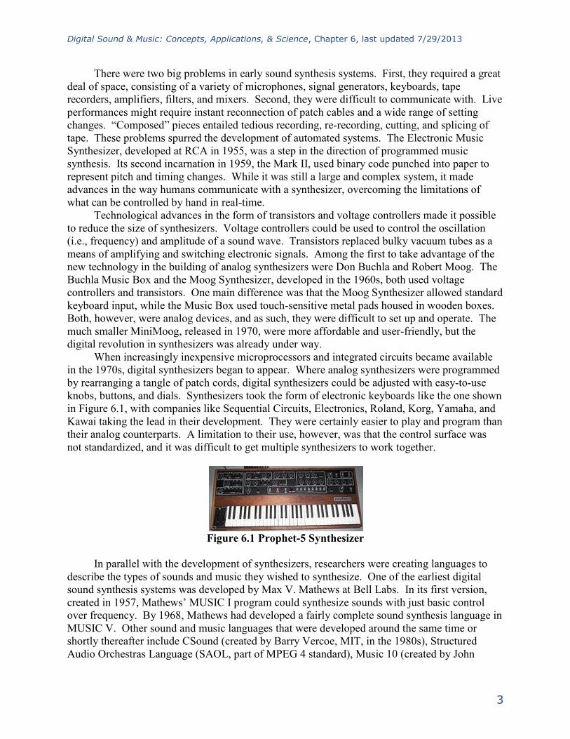
knobs, buttons, and dials. Synthesizers took the form of electronic keyboards like the one shown
in Figure 6.1, with companies like Sequential Circuits, Electronics, Roland, Korg, Yamaha, and
Kawai taking the lead in their development. They were certainly easier to play and program than
their analog counterparts. A limitation to their use, however, was that the control surface was
not standardized, and it was difficult to get multiple synthesizers to work together.
Figure 6.1 Prophet-5 Synthesizer
In parallel with the development of synthesizers, researchers were creating languages to
describe the types of sounds and music they wished to synthesize. One of the earliest digital
sound synthesis systems was developed by Max V. Mathews at Bell Labs. In its first version,
created in 1957, Mathews’ MUSIC I program could synthesize sounds with just basic control
over frequency. By 1968, Mathews had developed a fairly complete sound synthesis language in
MUSIC V. Other sound and music languages that were developed around the same time or
shortly thereafter include CSound (created by Barry Vercoe, MIT, in the 1980s), Structured
Audio Orchestras Language (SAOL, part of MPEG 4 standard), Music 10 (created by John

Digital Sound & Music: Concepts, Applications, & Science, Chapter 6, last updated 7/29/2013
4
Chowning, Stanford, in 1966), cmusic (created by F. Richard Moore, University of California
San Diego in the 1990s), and pcmusic (also created by F. Richard Moore).
In the early 1980s, led by Dave Smith from Sequential Circuits and Ikutaru Kakehashi
from Roland, a group of the major synthesizer manufacturers decided that it was in their mutual
interest to find a common language for their devices. Their collaboration resulted in the 1983
release of the MIDI 1.0 Detailed Specification. The original document defined only basic
instructions, things like how to play notes and control volume. Later revisions added messages
for greater control of synthesizers and branched out to messages controlling stage lighting.
General MIDI (1991) attempted to standardize the association between program numbers and
instruments synthesized. It also added new connection types (e.g., USB, FireWire, and wireless),
and new platforms such as mobile phones and video games.
This short history lays the ground for the two main topics to be covered in this chapter:
symbolic encoding of music and sound information – in particular, MIDI – and how this
encoding is translated into sound by digital sound synthesis. We begin with a definition of MIDI
and an explanation of how it differs from digital audio, after which we can take a closer look at
how MIDI commands are interpreted via sound synthesis.
MIDI Components 6.1.2MIDI (Musical Instrument Digital Interface) is a term that actually refers to a number of things:
A symbolic language of event-based messages frequently used to represent music
A standard interpretation of messages, including what instrument sounds and notes are
intended upon playback (although the messages can be interpreted to mean other things,
at the user’s discretion)
A type of physical connection between one digital device and another
Input and output ports that accommodate the MIDI connections, translating back and
forth between digital data to electrical voltages according to the MIDI protocol
A transmission protocol that specifies the order and type of data to be transferred from
one digital device to another
Let’s look at all of these associations in the context of a simple real-world example. (Refer to
the Preface for an overview of your DAW and MIDI setup.) A setup for recording and editing
MIDI on a computer commonly has these five components:
A means to input MIDI messages: a MIDI input device, such as a MIDI Keyboard or
MIDI controller. This could be something that looks like a piano keyboard, only it
doesn’t generate sound itself. Often MIDI keyboards have controller functions as well,
such as knobs, faders, and buttons, as shown in Figure 1.5 in Chapter 1. It’s also possible
to use your computer keyboard as an input device if you don’t have any other controller.
The MIDI input program on your computer may give you an interface on the computer
screen that looks like a piano keyboard, as shown in Figure 6.2.

Digital Sound & Music: Concepts, Applications, & Science, Chapter 6, last updated 7/29/2013
5
Figure 6.2 Software interface for MIDI controller from Apple Logic
A means to transmit MIDI messages: a cable connecting your computer and the MIDI
controller via MIDI ports or another data connection such as USB or FireWire.
A means to receive, record, and process MIDI messages: a MIDI sequencer, which is
software on your computer providing a user interface to capture, arrange, and manipulate
the MIDI data. The interfaces of two commonly used software sequencers – Logic (Mac-
based) and Cakewalk Sonar (Windows-based) are shown in Figures 1.29 and 1.30 of
Chapter 1. The interface of Reason (Mac or Windows) is shown in Figure 6.3.
A means to interpret MIDI messages
and create sound: either a hardware
or a software synthesizer. All three of
the sequencers pictured in the
aforementioned figures give you
access to a variety of software
synthesizers (soft synths, for short)
and instrument plug-ins (soft synths often created by third-party vendors). If you don’t
have a dedicated hardware of software synthesizer within your system, you may have to
resort to the soft synth supplied by your operating system. For example, Figure 6.4
shows that the only choice of synthesizer for that system setup is the Microsoft GS
Wavetable Synth. Some sound cards have hardware support for sound synthesis, so this
may be another option.
A means to do digital-to-analog conversion and listen to the sound: a sound card in the
computer or external audio interface connected to a set of loudspeakers or headphones.
Figure 6.3 Reason’s sequencer
Aside: We use the term synthesizer in a broad sense here, including samplers that produce sound from memory bands of
recorded samples. We’ll explain the distinction between synthesizers and samplers in more detail in Section 7.1.6.
Digital Sound & Music: Concepts, Applications, & Science, Chapter 6, last updated 7/29/2013
6
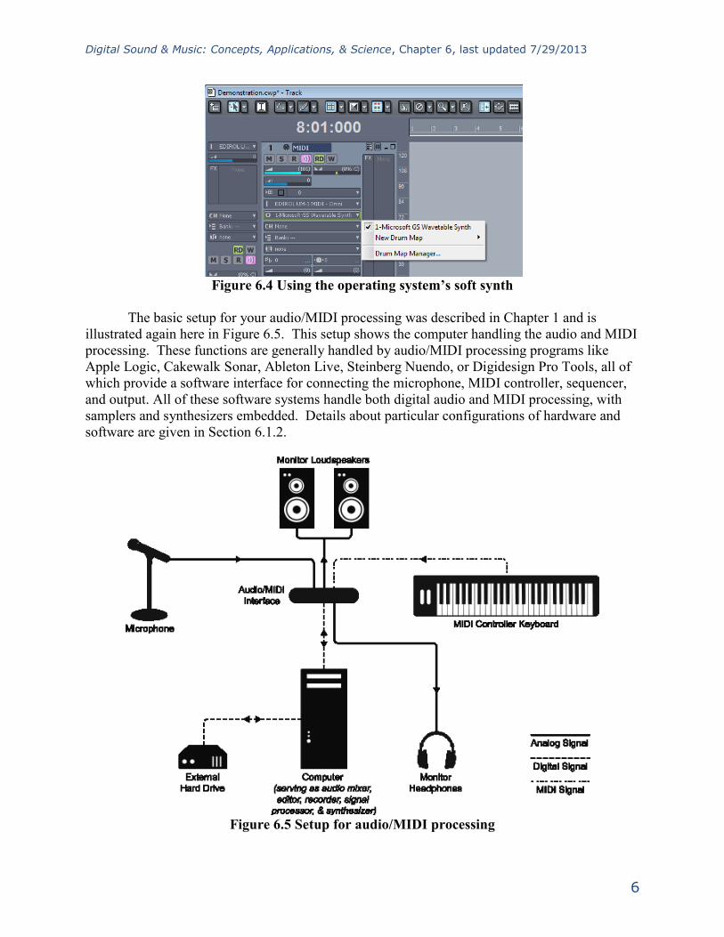
Figure 6.4 Using the operating system’s soft synth
The basic setup for your audio/MIDI processing was described in Chapter 1 and is
illustrated again here in Figure 6.5. This setup shows the computer handling the audio and MIDI
processing. These functions are generally handled by audio/MIDI processing programs like
Apple Logic, Cakewalk Sonar, Ableton Live, Steinberg Nuendo, or Digidesign Pro Tools, all of
which provide a software interface for connecting the microphone, MIDI controller, sequencer,
and output. All of these software systems handle both digital audio and MIDI processing, with
samplers and synthesizers embedded. Details about particular configurations of hardware and
software are given in Section 6.1.2.
Figure 6.5 Setup for audio/MIDI processing

Digital Sound & Music: Concepts, Applications, & Science, Chapter 6, last updated 7/29/2013
7
When you have your system properly connected and configured, you’re ready to go.
Now you can “arm” the sequencer for recording, press a key on the controller, and record that
note in the sequencer. Most likely pressing that key doesn’t even make a sound, since we
haven’t yet told the sound where to go. Your controller may look like a piano, but it’s really just
an input device sending a digital message to your computer in some agreed upon format. This is
the purpose of the MIDI transmission protocol. In order for the two devices to communicate, the
connection between them must be designed to transmit MIDI messages. For example, the cable
could be USB at the computer end and have dual 5-pin DIN connections at the keyboard end, as
shown in Figure 6.6. The message that is received by your MIDI sequencer is in a prescribed
MIDI format. In the sequencer, you can save this and any subsequent messages into a file. You
can also play the messages back and, depending on your settings, the notes upon playback can
sound like any instrument you choose from a wide variety of choices. It is the synthesizer that
turns the symbolic MIDI message into digital audio data and sends the data to the sound card to
be played.
Figure 6.6 5-pin DIN connection for MIDI
MIDI Data Compared to Digital Audio 6.1.3Consider how MIDI data differs from digital audio as described in Chapter 5. You aren’t
recording something through a microphone. MIDI keyboards don’t necessarily make a sound
when you strike a key on a piano keyboard-like controller, and they don’t function as stand-alone
instruments. There’s no sampling and quantization going on at all. Instead, the controller is
engineered to know that when a certain key is played, a symbolic message should be sent
detailing the performance information.
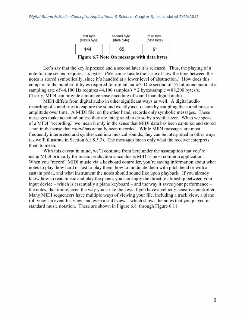
In the case of a key press, the MIDI message would convey the occurrence of a Note On,
followed by the note pitch played (e.g., middle C)
and the velocity with which it was struck. The
MIDI message generated by this action is only
three bytes long. It’s essentially just three
numbers, as shown in Figure 6.7. The first
byte is a value between 144 and 159. The
second and third bytes are values between 0 and 127. The fact that the first value is between 144
and 159 is what makes it identifiable by the receiver as a Note On message, and the fact that it is
a Note On message is what identifies the next two bytes as the specific note and velocity. A
Note Off message is handled similarly, with the first byte identifying the message as Note Off
and the second and third giving note and velocity information (which can be used to control note
decay).
Aside: Many systems interpret a Note On message with velocity 0 as “note off” and use this as an alternative to the Note Off
message.
Digital Sound & Music: Concepts, Applications, & Science, Chapter 6, last updated 7/29/2013
8
Figure 6.7 Note On message with data bytes
Let’s say that the key is pressed and a second later it is released. Thus, the playing of a
note for one second requires six bytes. (We can set aside the issue of how the time between the
notes is stored symbolically, since it’s handled at a lower level of abstraction.) How does this
compare to the number of bytes required for digital audio? One second of 16-bit mono audio at a
sampling rate of 44,100 Hz requires 44,100 samples/s * 2 bytes/sample = 88,200 bytes/s.
Clearly, MIDI can provide a more concise encoding of sound than digital audio.
MIDI differs from digital audio in other significant ways as well. A digital audio
recording of sound tries to capture the sound exactly as it occurs by sampling the sound pressure
amplitude over time. A MIDI file, on the other hand, records only symbolic messages. These
messages make no sound unless they are interpreted to do so by a synthesizer. When we speak
of a MIDI “recording,” we mean it only in the sense that MIDI data has been captured and stored
– not in the sense that sound has actually been recorded. While MIDI messages are most
frequently interpreted and synthesized into musical sounds, they can be interpreted in other ways
(as we’ll illustrate in Section 6.1.8.5.3). The messages mean only what the receiver interprets
them to mean.
With this caveat in mind, we’ll continue from here under the assumption that you’re
using MIDI primarily for music production since this is MIDI’s most common application.
When you “record” MIDI music via a keyboard controller, you’re saving information about what
notes to play, how hard or fast to play them, how to modulate them with pitch bend or with a
sustain pedal, and what instrument the notes should sound like upon playback. If you already
know how to read music and play the piano, you can enjoy the direct relationship between your
input device – which is essentially a piano keyboard – and the way it saves your performance –
the notes, the timing, even the way you strike the keys if you have a velocity-sensitive controller.
Many MIDI sequencers have multiple ways of viewing your file, including a track view, a piano
roll view, an event list view, and even a staff view – which shows the notes that you played in
standard music notation. These are shown in Figure 6.8 through Figure 6.11.

Digital Sound & Music: Concepts, Applications, & Science, Chapter 6, last updated 7/29/2013
9
Figure 6.8 Track view in Cakewalk Sonar

Digital Sound & Music: Concepts, Applications, & Science, Chapter 6, last updated 7/29/2013
10
Figure 6.9 Piano roll view in Cakewalk Sonar
Figure 6.10 Staff view in Cakewalk Sonar
Figure 6.11 Event list view in Cakewalk Sonar
Digital Sound & Music: Concepts, Applications, & Science, Chapter 6, last updated 7/29/2013
11
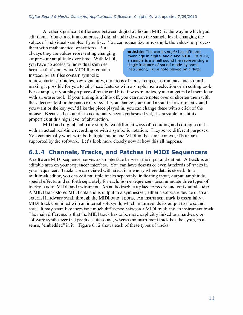
Another significant difference between digital audio and MIDI is the way in which you
edit them. You can edit uncompressed digital audio down to the sample level, changing the
values of individual samples if you like. You can requantize or resample the values, or process
them with mathematical operations. But
always they are values representing changing
air pressure amplitude over time. With MIDI,
you have no access to individual samples,
because that’s not what MIDI files contain.
Instead, MIDI files contain symbolic
representations of notes, key signatures, durations of notes, tempo, instruments, and so forth,
making it possible for you to edit these features with a simple menu selection or an editing tool.
For example, if you play a piece of music and hit a few extra notes, you can get rid of them later
with an eraser tool. If your timing is a little off, you can move notes over or shorten them with
the selection tool in the piano roll view. If you change your mind about the instrument sound
you want or the key you’d like the piece played in, you can change these with a click of the
mouse. Because the sound has not actually been synthesized yet, it’s possible to edit its
properties at this high level of abstraction.
MIDI and digital audio are simply two different ways of recording and editing sound –
with an actual real-time recording or with a symbolic notation. They serve different purposes.
You can actually work with both digital audio and MIDI in the same context, if both are
supported by the software. Let’s look more closely now at how this all happens.
Channels, Tracks, and Patches in MIDI Sequencers 6.1.4A software MIDI sequencer serves as an interface between the input and output. A track is an
editable area on your sequencer interface. You can have dozens or even hundreds of tracks in
your sequencer. Tracks are associated with areas in memory where data is stored. In a
multitrack editor, you can edit multiple tracks separately, indicating input, output, amplitude,
special effects, and so forth separately for each. Some sequencers accommodate three types of
tracks: audio, MIDI, and instrument. An audio track is a place to record and edit digital audio.
A MIDI track stores MIDI data and is output to a synthesizer, either a software device or to an
external hardware synth through the MIDI output ports. An instrument track is essentially a
MIDI track combined with an internal soft synth, which in turn sends its output to the sound
card. It may seem like there isn't much difference between a MIDI track and an instrument track.
The main difference is that the MIDI track has to be more explicitly linked to a hardware or
software synthesizer that produces its sound, whereas an instrument track has the synth, in a
sense, "embedded" in it. Figure 6.12 shows each of these types of tracks.
Aside: The word sample has different meanings in digital audio and MIDI. In MIDI, a sample is a small sound file representing a single instance of sound made by some instrument, like a note played on a flute.

Digital Sound & Music: Concepts, Applications, & Science, Chapter 6, last updated 7/29/2013
12
Figure 6.12 Three types of tracks in Logic
A channel is a communication path. According to the MIDI standard, a single MIDI
cable can transmit up to 16 channels. Without knowing the details of how this is engineered, you
can just think of it abstractly as 16 separate lines of communication.
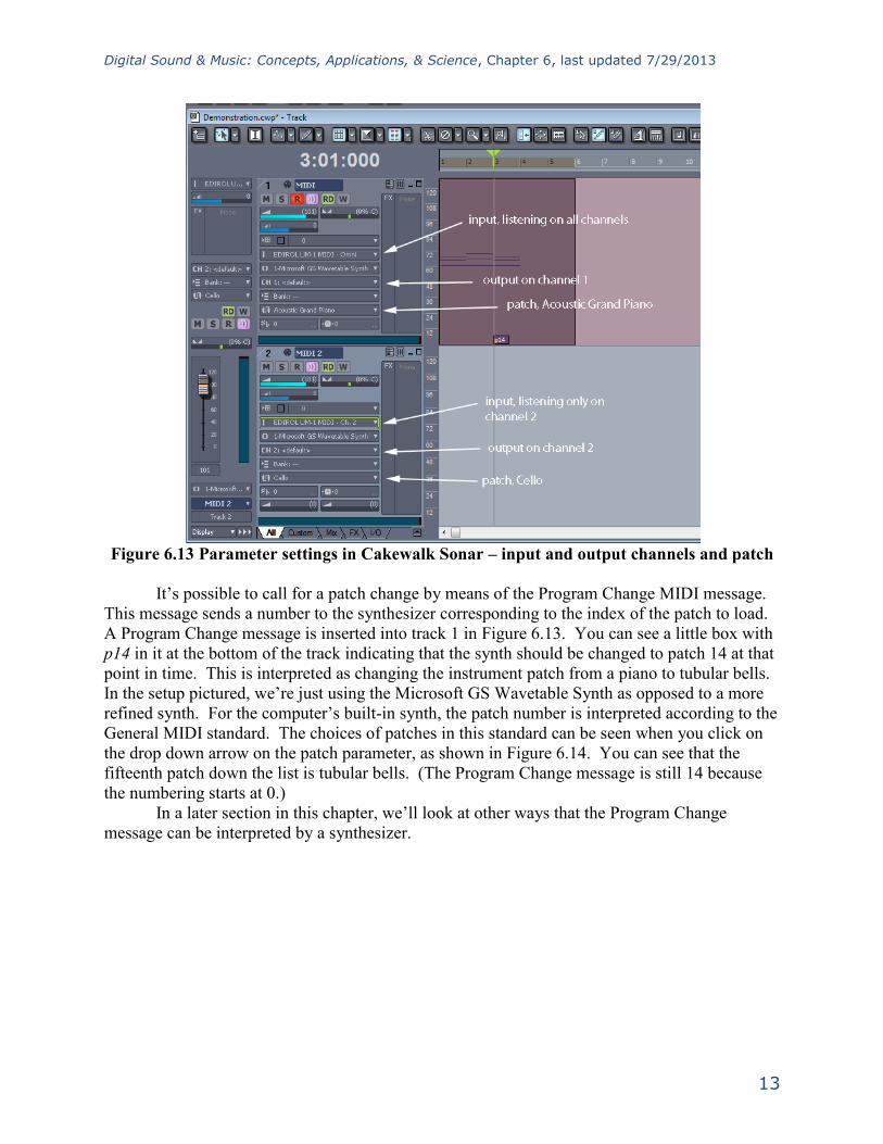
There are both input and output channels. An incoming message can tell what channel it
is to be transmitted on, and this can route the message to a particular device. In the sequencer
pictured in Figure 6.13, track 1 is listening on all channels, indicated by the word OMNI. Track
2 is listening only on Channel 2.
The output channels are pointed out in the figure, also. When the message is sent out to
the synthesizer, different channels can correspond to different instrument sounds. The parameter
setting marked with a patch cord icon is the patch. A patch is a message to the synthesizer – just
a number that indicates how the synthesizer is to operate as it creates sounds. The synthesizer
can be programmed in different ways to respond to the patch setting. Sometimes the patch refers
to a setting you’ve stored in the synthesizer that tells it what kinds of waveforms to combine or
what kind of special effects to apply. In the example shown in Figure 6.13, however, the patch is
simply interpreted as the choice of instrument that the user has chosen for the track. Track 1 is
outputting on Channel 1 with the patch set to Acoustic Grand Piano. Track 2 is outputting on
Channel 2 with the patch set to Cello.
Digital Sound & Music: Concepts, Applications, & Science, Chapter 6, last updated 7/29/2013
13
Figure 6.13 Parameter settings in Cakewalk Sonar – input and output channels and patch
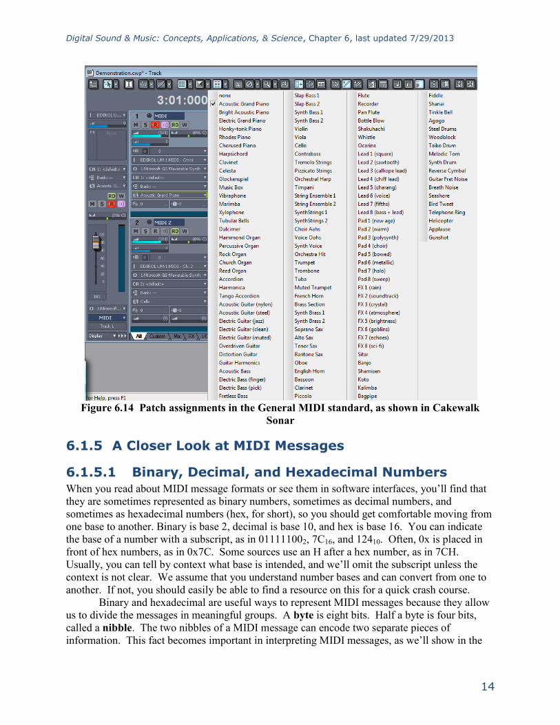
It’s possible to call for a patch change by means of the Program Change MIDI message.
This message sends a number to the synthesizer corresponding to the index of the patch to load.
A Program Change message is inserted into track 1 in Figure 6.13. You can see a little box with
p14 in it at the bottom of the track indicating that the synth should be changed to patch 14 at that
point in time. This is interpreted as changing the instrument patch from a piano to tubular bells.
In the setup pictured, we’re just using the Microsoft GS Wavetable Synth as opposed to a more
refined synth. For the computer’s built-in synth, the patch number is interpreted according to the
General MIDI standard. The choices of patches in this standard can be seen when you click on
the drop down arrow on the patch parameter, as shown in Figure 6.14. You can see that the
fifteenth patch down the list is tubular bells. (The Program Change message is still 14 because
the numbering starts at 0.)
In a later section in this chapter, we’ll look at other ways that the Program Change
message can be interpreted by a synthesizer.
Digital Sound & Music: Concepts, Applications, & Science, Chapter 6, last updated 7/29/2013
14
Figure 6.14 Patch assignments in the General MIDI standard, as shown in Cakewalk
Sonar
A Closer Look at MIDI Messages 6.1.5
Binary, Decimal, and Hexadecimal Numbers 6.1.5.1When you read about MIDI message formats or see them in software interfaces, you’ll find that
they are sometimes represented as binary numbers, sometimes as decimal numbers, and
sometimes as hexadecimal numbers (hex, for short), so you should get comfortable moving from
one base to another. Binary is base 2, decimal is base 10, and hex is base 16. You can indicate
the base of a number with a subscript, as in 011111002, 7C16, and 12410. Often, 0x is placed in
front of hex numbers, as in 0x7C. Some sources use an H after a hex number, as in 7CH.
Usually, you can tell by context what base is intended, and we’ll omit the subscript unless the
context is not clear. We assume that you understand number bases and can convert from one to
another. If not, you should easily be able to find a resource on this for a quick crash course.
Binary and hexadecimal are useful ways to represent MIDI messages because they allow
us to divide the messages in meaningful groups. A byte is eight bits. Half a byte is four bits,
called a nibble. The two nibbles of a MIDI message can encode two separate pieces of
information. This fact becomes important in interpreting MIDI messages, as we’ll show in the

Digital Sound & Music: Concepts, Applications, & Science, Chapter 6, last updated 7/29/2013
15
next section. In both the binary and hexadecimal representations, we can see the two nibbles as
two separate pieces of information, which isn’t possible in decimal notation.
A convenient way to move from hexadecimal to binary is to translate each nibble into
four bits and concatenate them into a byte. For example, in the case of 0x7C, the 7 in
hexadecimal becomes 0111 in binary. The C in hexadecimal becomes 1100 in binary. Thus
0x7C is 01111100 in binary. (Note that the symbols A through F correspond to decimal values
10 through 15, respectively, in hexadecimal notation.)
MIDI Messages, Types, and Formats 6.1.5.2In Section 6.1.3, we showed you an example of a commonly used MIDI message, Note On, but
now let’s look at the general protocol.
MIDI messages consist of one or more bytes. The first byte of each message is a status
byte, identifying the type of message being sent. This is followed by 0 or more data bytes,
depending on the type of message. Data bytes give more information related to the type of
message, like note pitch and velocity related to Note On.
All status bytes have a 1 as their most significant bit, and all data bytes have a 0. A byte
with a 1 in its most significant bit has a value of at least 128. That is, 10000000 in binary is
equal to 128 in decimal, and the maximum value that an 8 bit binary number can have
(11111111) is the decimal value 255. Thus, status bytes always have a decimal value between
128 and 255. This is 10000000 through 11111111 in binary and 80 through FF in hex.
MIDI messages can be divided into two main categories: Channel messages and System
messages. Channel messages contain the channel number. They can be further subdivided into
voice and mode messages. Voice messages include Note On, Note Off, Polyphonic Key
Pressure, Control Change, Program Change, Channel Pressure/Aftertouch, and Pitch Bend. A
mode indicates how a device is to respond to messages on a certain channel. A device might be
set to respond to all MIDI channels (called Omni mode), or it might be instructed to respond to
polyphonic messages or only monophonic ones. Polyphony involves playing more than one
note at the same time.
System messages are sent to the whole system rather than a particular channel. They can
be subdivided into Real Time, Common, and System Exclusive messages (SysEx). The System
Common messages include Tune Request, Song Select, and Song Position Pointer. The system
real time messages include Timing Clock, Start, Stop, Continue, Active Sensing, and System
Reset. SysEx messages can be defined by manufacturers in their own way to communicate
things that are not part of the MIDI standard. The types of messages are diagrammed in Figure
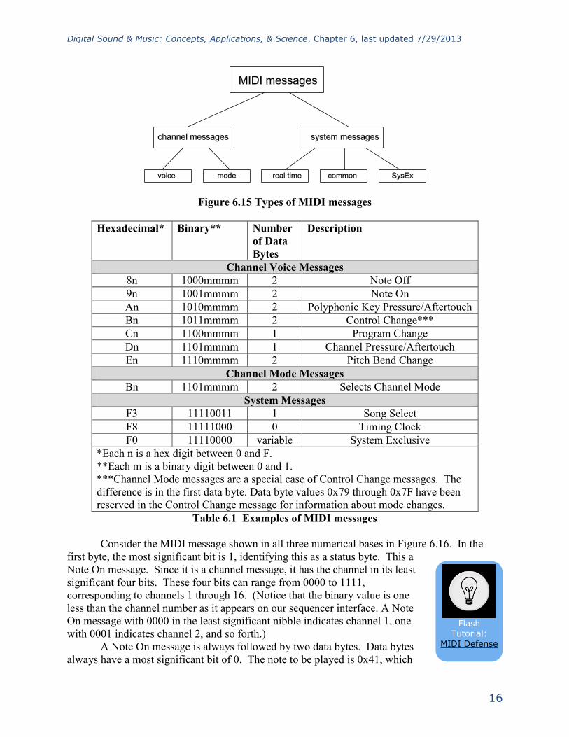
6.15. A few of these messages are shown in Table 6.1.
Digital Sound & Music: Concepts, Applications, & Science, Chapter 6, last updated 7/29/2013
16
Figure 6.15 Types of MIDI messages
Hexadecimal* Binary** Number
of Data
Bytes
Description
Channel Voice Messages
8n 1000mmmm 2 Note Off
9n 1001mmmm 2 Note On
An 1010mmmm 2 Polyphonic Key Pressure/Aftertouch
Bn 1011mmmm 2 Control Change***
Cn 1100mmmm 1 Program Change
Dn 1101mmmm 1 Channel Pressure/Aftertouch
En 1110mmmm 2 Pitch Bend Change
Channel Mode Messages
Bn 1101mmmm 2 Selects Channel Mode
System Messages
F3 11110011 1 Song Select
F8 11111000 0 Timing Clock
F0 11110000 variable System Exclusive
*Each n is a hex digit between 0 and F.
**Each m is a binary digit between 0 and 1.
***Channel Mode messages are a special case of Control Change messages. The
difference is in the first data byte. Data byte values 0x79 through 0x7F have been
reserved in the Control Change message for information about mode changes.
Table 6.1 Examples of MIDI messages
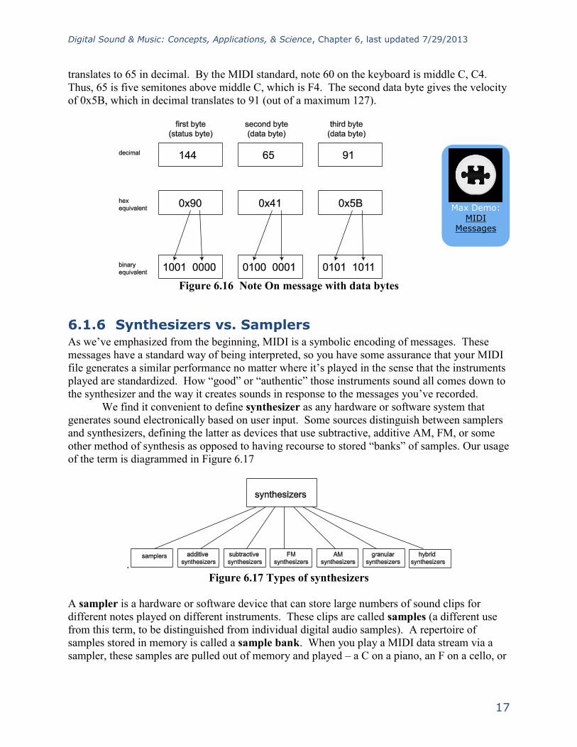
Consider the MIDI message shown in all three numerical bases in Figure 6.16. In the
first byte, the most significant bit is 1, identifying this as a status byte. This a
Note On message. Since it is a channel message, it has the channel in its least
significant four bits. These four bits can range from 0000 to 1111,
corresponding to channels 1 through 16. (Notice that the binary value is one
less than the channel number as it appears on our sequencer interface. A Note
On message with 0000 in the least significant nibble indicates channel 1, one
with 0001 indicates channel 2, and so forth.)
A Note On message is always followed by two data bytes. Data bytes
always have a most significant bit of 0. The note to be played is 0x41, which
Flash
Tutorial: MIDI Defense
Digital Sound & Music: Concepts, Applications, & Science, Chapter 6, last updated 7/29/2013
17
translates to 65 in decimal. By the MIDI standard, note 60 on the keyboard is middle C, C4.
Thus, 65 is five semitones above middle C, which is F4. The second data byte gives the velocity
of 0x5B, which in decimal translates to 91 (out of a maximum 127).
Figure 6.16 Note On message with data bytes
Synthesizers vs. Samplers 6.1.6As we’ve emphasized from the beginning, MIDI is a symbolic encoding of messages. These
messages have a standard way of being interpreted, so you have some assurance that your MIDI
file generates a similar performance no matter where it’s played in the sense that the instruments
played are standardized. How “good” or “authentic” those instruments sound all comes down to
the synthesizer and the way it creates sounds in response to the messages you’ve recorded.
We find it convenient to define synthesizer as any hardware or software system that
generates sound electronically based on user input. Some sources distinguish between samplers
and synthesizers, defining the latter as devices that use subtractive, additive AM, FM, or some
other method of synthesis as opposed to having recourse to stored “banks” of samples. Our usage
of the term is diagrammed in Figure 6.17
.
Figure 6.17 Types of synthesizers
A sampler is a hardware or software device that can store large numbers of sound clips for
different notes played on different instruments. These clips are called samples (a different use
from this term, to be distinguished from individual digital audio samples). A repertoire of
samples stored in memory is called a sample bank. When you play a MIDI data stream via a
sampler, these samples are pulled out of memory and played – a C on a piano, an F on a cello, or
Max Demo:
MIDI Messages

Digital Sound & Music: Concepts, Applications, & Science, Chapter 6, last updated 7/29/2013
18
whatever is asked for in the MIDI messages. Because the sounds played are actual recordings of
musical instruments, they sound realistic.
The NN-XT sampler from Reason is pictured in Figure 6.18. You can see that there are
WAV files for piano notes, but there isn’t a WAV file for every single note on the keyboard. In
a method called multisampling, one audio sample can be used to create the sound of a number
of neighboring ones. The notes covered by a single audio sample constitute a zone. The sampler
is able to use a single sample for multiple notes by pitch-shifting the sample up or down by an
appropriate number of semitones. The pitch can’t be stretched too far, however, without
eventually distorting the timbre and amplitude envelope of the note such that the note no longer
sounds like the instrument and frequency it’s supposed to be. Higher and lower notes can be
stretched more without our minding it, since our ears are less sensitive in these areas.
There can be more than one audio sample associated with a single note, also. For
example, a single note can be represented by three samples where notes are played at three
different velocities – high, medium, and low. The same note has a different timbre and
amplitude envelope depending on the velocity with which it is played, so having more than one
sample for a note results in more realistic sounds.
Samplers can also be used for sounds that aren’t necessarily recreations of traditional
instruments. It’s possible to assign whatever sound file you want to the notes on the keyboard.
You can create your own entirely new sound bank, or you can purchase additional sound
libraries and install them (depending on the features offered by your sampler). Sample libraries
come in a variety of formats. Some contain raw audio WAV or AIFF files which have to be
mapped individually to keys. Others are in special sampler file formats that are compressed and
automatically installable.
Figure 6.18 The NN-XT sampler from Reason
A synthesizer, if you use this word in the strictest sense, doesn’t have a huge memory
bank of samples. Instead, it creates sound more dynamically. It could do this by beginning with
basic waveforms like sawtooth, triangle, or square waves and performing mathematical
Digital Sound & Music: Concepts, Applications, & Science, Chapter 6, last updated 7/29/2013
19
operations on them to alter their shapes. The
user controls this process by knobs, dials,
sliders, and other input controls on the
control surface of the synthesizer – whether
this is a hardware synthesizer or a soft synth.
Under the hood, a synthesizer could be using
a variety of mathematical methods, including
additive, subtractive, FM, AM, or wavetable
synthesis, or physical modeling. We’ll
examine some of these methods in more
detail in Section 6.3.1. This method of
creating sounds may not result in making the
exact sounds of a musical instrument.
Musical instruments are complex structures, and it’s difficult to model their timbre and
amplitude envelopes exactly. However, synthesizers can create novel sounds that we don’t
often, if ever, encounter in nature or music, offering creative possibilities to innovative
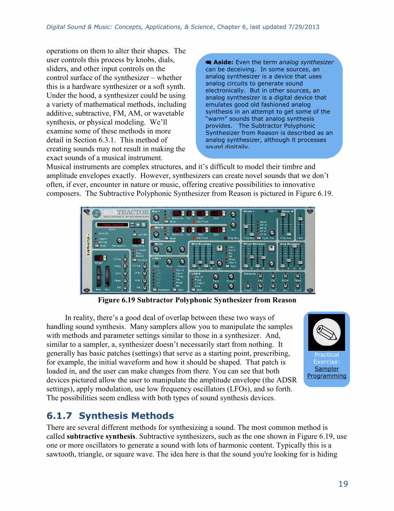
composers. The Subtractive Polyphonic Synthesizer from Reason is pictured in Figure 6.19.
Figure 6.19 Subtractor Polyphonic Synthesizer from Reason
In reality, there’s a good deal of overlap between these two ways of
handling sound synthesis. Many samplers allow you to manipulate the samples
with methods and parameter settings similar to those in a synthesizer. And,
similar to a sampler, a, synthesizer doesn’t necessarily start from nothing. It
generally has basic patches (settings) that serve as a starting point, prescribing,
for example, the initial waveform and how it should be shaped. That patch is
loaded in, and the user can make changes from there. You can see that both
devices pictured allow the user to manipulate the amplitude envelope (the ADSR
settings), apply modulation, use low frequency oscillators (LFOs), and so forth.
The possibilities seem endless with both types of sound synthesis devices.
Synthesis Methods 6.1.7There are several different methods for synthesizing a sound. The most common method is
called subtractive synthesis. Subtractive synthesizers, such as the one shown in Figure 6.19, use
one or more oscillators to generate a sound with lots of harmonic content. Typically this is a
sawtooth, triangle, or square wave. The idea here is that the sound you're looking for is hiding
Practical Exercise: Sampler
Programming
Aside: Even the term analog synthesizer
can be deceiving. In some sources, an analog synthesizer is a device that uses analog circuits to generate sound electronically. But in other sources, an analog synthesizer is a digital device that emulates good old fashioned analog synthesis in an attempt to get some of the
“warm” sounds that analog synthesis provides. The Subtractor Polyphonic Synthesizer from Reason is described as an analog synthesizer, although it processes sound digitally.

Digital Sound & Music: Concepts, Applications, & Science, Chapter 6, last updated 7/29/2013
20
somewhere in all those harmonics. All you need to do is subtract the harmonics you don’t want,
and you’ll expose the properties of the sound you're trying to synthesize. The actual subtraction
is done using a filter. Further shaping of the sound is accomplished by modifying the filter
parameters over time using envelopes or low frequency oscillators. If you can learn all the
components of a subtractive synthesize,r you're well on your way to understanding the other
synthesis methods because they all use similar components.
The opposite of subtractive synthesis is additive synthesis. This method involves
building the sound you're looking for using multiple sine waves. The theory here is that all
sounds are made of individual sine waves that come together to make a complex tone. While you
can theoretically create any sound you want using additive synthesis, this is a very cumbersome
method of synthesis and is not commonly used.
Another common synthesis method is called frequency modulation (FM) synthesis.
This method of synthesis works by using two oscillators with one oscillator modulating the
signal from the other. These two oscillators are called the modulator and the carrier. Some
really interesting sounds can be created with this synthesis method that would be difficult to
achieve with subtractive synthesis. The Yamaha DX7 synthesizer is probably the most popular
FM synthesizer and also holds the title of the first commercially available digital synthesizer.
Figure 6.20 shows an example of an FM synthesizer from Logic Pro.
Figure 6.20 A FM synthesizer from Logic Pro
Wavetable synthesis is a synthesis method where several different single-cycle
waveforms are strung together in what’s called a wavetable. When you play a note on the
keyboard, you're triggering a predetermined sequence of waves that transition smoothly between
each other. This synthesis method is not very good at mimicking acoustic instruments, but it's
very good at creating artificial sounds that are constantly in motion.
Other synthesis methods include granular synthesis, physical modeling synthesis, and
phase distortion synthesis. If you’re just starting out with synthesizers, begin with a simple
Digital Sound & Music: Concepts, Applications, & Science, Chapter 6, last updated 7/29/2013
21
subtractive synthesizer and then move on to a FM synthesizer. Once you’ve run out of sounds
you can create using those two synthesis methods, you’ll be ready to start experimenting with
some of these other synthesis methods.
Synthesizer Components 6.1.8
Presets 6.1.8.1Now let’s take a closer look at synthesizers. In this section, we’re referring to synthesizers in the
strict sense of the word – those that can be programmed to create sounds dynamically, as
opposed to using recorded samples of real instruments. Synthesizer programming entails
selecting an initial patch or waveform, filtering it, amplifying it, applying envelopes, applying
low frequency oscillators to shape the amplitude or frequency changes, and so forth, as we’ll
describe below.
There are many different forms of sound synthesis, but they all use the same basic tools
to generate the sounds. The difference is how the tools are used and connected together. In most
cases, the software synthesizer comes with a large library of pre-built patches that configure the
synthesizer to make various sounds. In your own work, you’ll probably use the presets as a
starting point and modify the patches to your liking. Once you learn to master the tools, you can
start building your own patches from scratch to create any sound you can imagine.
Sound Generator 6.1.8.2The first object in the audio path of any synthesizer is the sound generator. Regardless of the
synthesis method being used, you have to start by creating some sort of sound that is then shaped
into the specific sound you’re looking for. In most cases, the sound generator is made up of one
or more oscillators that create simple sounds like sine, sawtooth, triangle, and square waves. The
sound generator might also consist of a noise generator that plays pink noise or white noise. You
might also see a wavetable oscillator that can play a pre-recorded complex shape. If your
synthesizer has multiple sound generators, there is also some sort of mixer that merges all the
sounds together. Depending on the synthesis method being used, you may also have an option to
decide how the sounds are combined (i.e. through addition, multiplication, modulation, etc.).
Because synthesizers are most commonly used as musical instruments, there typically is a
control on the oscillator that adjusts the frequency of the sound that is generated. This frequency
can usually be changed remotely over time but typically, you choose some sort of starting point
and any pitch changes are applied relative to the starting frequency.
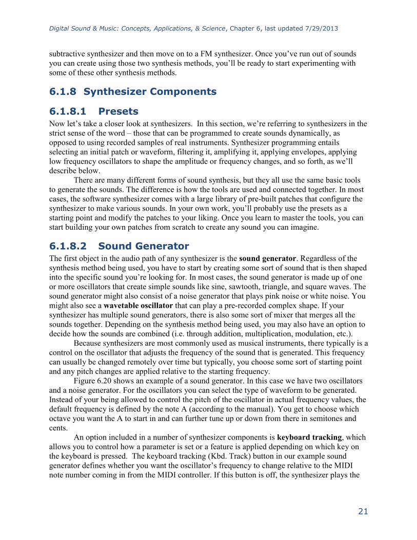
Figure 6.20 shows an example of a sound generator. In this case we have two oscillators
and a noise generator. For the oscillators you can select the type of waveform to be generated.
Instead of your being allowed to control the pitch of the oscillator in actual frequency values, the
default frequency is defined by the note A (according to the manual). You get to choose which
octave you want the A to start in and can further tune up or down from there in semitones and
cents.
An option included in a number of synthesizer components is keyboard tracking, which
allows you to control how a parameter is set or a feature is applied depending on which key on
the keyboard is pressed. The keyboard tracking (Kbd. Track) button in our example sound
generator defines whether you want the oscillator’s frequency to change relative to the MIDI
note number coming in from the MIDI controller. If this button is off, the synthesizer plays the

Digital Sound & Music: Concepts, Applications, & Science, Chapter 6, last updated 7/29/2013
22
same frequency regardless of the note played on the MIDI controller. The Phase, FM, Mix, and
Mode controls determine the way these two oscillators interact with each other.
Figure 6.21 Example of a sound generator in a synthesizer
Filters 6.1.8.3A filter is another object that is often found in the audio path. A filter is an object that modifies
the amplitude of specified frequencies in the audio signal. There are several types of filters. In
this section, we describe the basic features of filters most commonly found in synthesizers. For
more detailed information on filters, see Chapter 7.
Low-pass filters attempt to remove all frequencies above a certain point defined by the
filter cutoff frequency. There is always a slope to the filter that defines the rate at which the
frequencies are attenuated above the cutoff frequency. This is often called the filter order. A
first order filter attenuates frequencies above the cutoff frequency at the rate of 6 dB per octave.
If your cutoff frequency is 1 kHz, a first order filter attenuates 2 kHz by 6dB below the cutoff
frequency, 4 kHz by 12 dB, 8 kHz by 18 dB, etc. A second order filter attenuates 12 dB per
octave, a third order filter is 18 dB per octave, and a fourth order is 24 dB per octave. In some
cases, the filter order is fixed, but more sophisticated filters allow you to choose the filter order
that is the best fit for the sound you’re looking for. The cutoff frequency is typically the
frequency that has been attenuated 6 dB from the level of the frequencies that are unaffected by
the filter. The space between the cutoff frequency and frequencies that are not affected by the
filter is called the filter typography. The typography can be shaped by the filter’s resonance
control. Increasing the filter resonance creates a boost in the frequencies near the cutoff
frequency.
High-pass filters are the opposite of low-pass. Instead of removing all the frequencies
above a certain point, a high-pass filter removes all the frequencies below a certain point. A
high-pass filter has a cutoff frequency, filter order, and resonance control just like the low-pass
filter.
Bandpass filters are a combination of a high-pass and low-pass filter. A bandpass filter
has a low cutoff frequency and a high cutoff frequency with filter order and resonance controls
for each. In some cases, a bandpass filter is implemented with a fixed bandwidth or range of
frequencies between the two cutoff frequencies. This simplifies the number of controls needed
because you simply need to define a center frequency that positions the bandpass at the desired
location in the frequency spectrum.
Digital Sound & Music: Concepts, Applications, & Science, Chapter 6, last updated 7/29/2013
23
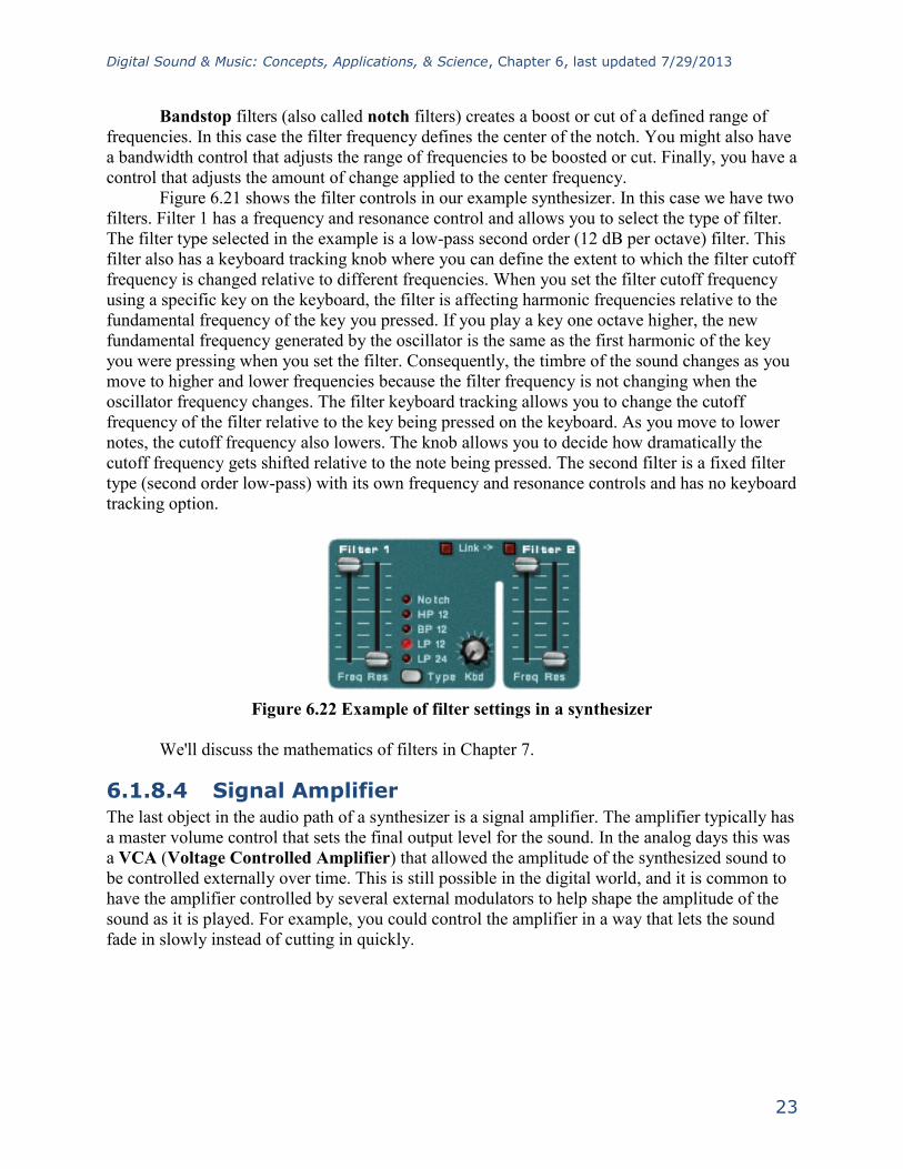
Bandstop filters (also called notch filters) creates a boost or cut of a defined range of
frequencies. In this case the filter frequency defines the center of the notch. You might also have
a bandwidth control that adjusts the range of frequencies to be boosted or cut. Finally, you have a
control that adjusts the amount of change applied to the center frequency.
Figure 6.21 shows the filter controls in our example synthesizer. In this case we have two
filters. Filter 1 has a frequency and resonance control and allows you to select the type of filter.
The filter type selected in the example is a low-pass second order (12 dB per octave) filter. This
filter also has a keyboard tracking knob where you can define the extent to which the filter cutoff
frequency is changed relative to different frequencies. When you set the filter cutoff frequency
using a specific key on the keyboard, the filter is affecting harmonic frequencies relative to the
fundamental frequency of the key you pressed. If you play a key one octave higher, the new
fundamental frequency generated by the oscillator is the same as the first harmonic of the key
you were pressing when you set the filter. Consequently, the timbre of the sound changes as you
move to higher and lower frequencies because the filter frequency is not changing when the
oscillator frequency changes. The filter keyboard tracking allows you to change the cutoff
frequency of the filter relative to the key being pressed on the keyboard. As you move to lower
notes, the cutoff frequency also lowers. The knob allows you to decide how dramatically the
cutoff frequency gets shifted relative to the note being pressed. The second filter is a fixed filter
type (second order low-pass) with its own frequency and resonance controls and has no keyboard
tracking option.
Figure 6.22 Example of filter settings in a synthesizer
We'll discuss the mathematics of filters in Chapter 7.
Signal Amplifier 6.1.8.4The last object in the audio path of a synthesizer is a signal amplifier. The amplifier typically has
a master volume control that sets the final output level for the sound. In the analog days this was
a VCA (Voltage Controlled Amplifier) that allowed the amplitude of the synthesized sound to
be controlled externally over time. This is still possible in the digital world, and it is common to
have the amplifier controlled by several external modulators to help shape the amplitude of the
sound as it is played. For example, you could control the amplifier in a way that lets the sound
fade in slowly instead of cutting in quickly.

Digital Sound & Music: Concepts, Applications, & Science, Chapter 6, last updated 7/29/2013
24
Figure 6.23 Master volume controller for the signal amplifier in a synthesizer
Modulation 6.1.8.5Modulation is the process of changing a shape of a waveform over time. This is done by
continuously changing one of the parameters that defines the waveform by multiplying it by
some coefficient. All the major parameters that define a waveform can be modulated, including
its frequency, amplitude, and phase. A graph of the coefficients by which the waveform is
modified shows us the shape of the modulation over time. This graph is sometimes referred to as
an envelope that is imposed over the chosen parameter, giving it a continuously changing shape.
The graph might correspond to a continuous function, like a sine, triangle, square, or sawtooth.
Alternative, the graph might represent a more complex function, like the ADSR envelope
illustrated in Figure 6.25 illustrates a particular type of envelope, called ADSR.
We'll see look at mathematics of amplitude, phase, and frequency modulation in Section
3. For now, we'll focus on LFOs and ADSR envelopes, commonly-used tools in synthesizers.
LFO 6.1.8.6LFO stands for low frequency oscillator. An LFO is simply an oscillator just like the ones
found in the sound generator section of the synthesizer. The difference here is that the LFO is not
part of the audio path of the synthesizer. In other words, you can’t hear the frequency generated
by the LFO. Even if the LFO was put into the audio path, it oscillates at frequencies well below
the range of human hearing so it isn't heard anyway. A LFO oscillates anywhere from 10 Hz
down to a fraction of a Hertz.
LFO’s are used like envelopes to modulate parameters of the synthesizer over time.
Typically you can choose from several different waveforms. For example, you can use an LFO
with a sinusoidal shape to change the pitch of the oscillator over time, creating a vibrato effect.
As the wave moves up and down, the pitch of the oscillator follows. You can also use an LFO to
control the sound amplitude over time to create a pulsing effect.
Figure 6.25 shows the LFO controls on a synthesizer. The Waveform button toggles the
LFO between one of six different waveforms. The Dest button toggles through a list of
destination parameters for the LFO. Currently, the LFO is set to create a triangle wave and apply
it to the pitch of Oscillators 1 and 2. The Rate knob defines the frequency of the LFO and the
Amount knob defines the amplitude of the wave or the amount of modulation that is applied. A
higher amount creates a more dramatic change to the destination parameter. When the Sync
button is engaged, the LFO frequency is synchronized to the incoming tempo for your song
based on a division defined by the Rate knob such as a quarter note or a half note.
Digital Sound & Music: Concepts, Applications, & Science, Chapter 6, last updated 7/29/2013
25
Figure 6.24 LFO controls on a synthesizer
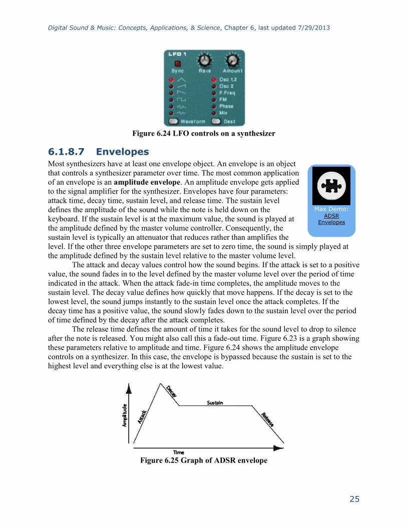
Envelopes 6.1.8.7Most synthesizers have at least one envelope object. An envelope is an object
that controls a synthesizer parameter over time. The most common application
of an envelope is an amplitude envelope. An amplitude envelope gets applied
to the signal amplifier for the synthesizer. Envelopes have four parameters:
attack time, decay time, sustain level, and release time. The sustain level
defines the amplitude of the sound while the note is held down on the
keyboard. If the sustain level is at the maximum value, the sound is played at
the amplitude defined by the master volume controller. Consequently, the
sustain level is typically an attenuator that reduces rather than amplifies the
level. If the other three envelope parameters are set to zero time, the sound is simply played at
the amplitude defined by the sustain level relative to the master volume level.
The attack and decay values control how the sound begins. If the attack is set to a positive
value, the sound fades in to the level defined by the master volume level over the period of time
indicated in the attack. When the attack fade-in time completes, the amplitude moves to the
sustain level. The decay value defines how quickly that move happens. If the decay is set to the
lowest level, the sound jumps instantly to the sustain level once the attack completes. If the
decay time has a positive value, the sound slowly fades down to the sustain level over the period
of time defined by the decay after the attack completes.
The release time defines the amount of time it takes for the sound level to drop to silence
after the note is released. You might also call this a fade-out time. Figure 6.23 is a graph showing
these parameters relative to amplitude and time. Figure 6.24 shows the amplitude envelope
controls on a synthesizer. In this case, the envelope is bypassed because the sustain is set to the
highest level and everything else is at the lowest value.
Figure 6.25 Graph of ADSR envelope
Max Demo:
ADSR Envelopes
Digital Sound & Music: Concepts, Applications, & Science, Chapter 6, last updated 7/29/2013
26
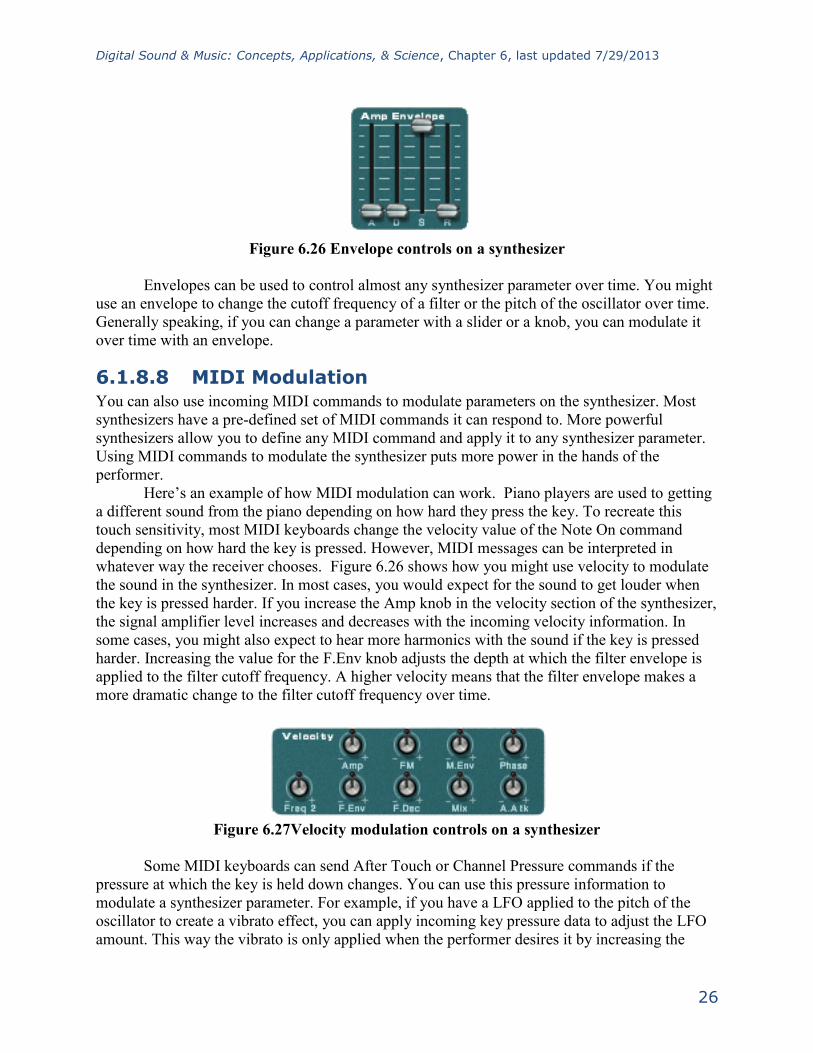
Figure 6.26 Envelope controls on a synthesizer
Envelopes can be used to control almost any synthesizer parameter over time. You might
use an envelope to change the cutoff frequency of a filter or the pitch of the oscillator over time.
Generally speaking, if you can change a parameter with a slider or a knob, you can modulate it
over time with an envelope.
MIDI Modulation 6.1.8.8You can also use incoming MIDI commands to modulate parameters on the synthesizer. Most
synthesizers have a pre-defined set of MIDI commands it can respond to. More powerful
synthesizers allow you to define any MIDI command and apply it to any synthesizer parameter.
Using MIDI commands to modulate the synthesizer puts more power in the hands of the
performer.
Here’s an example of how MIDI modulation can work. Piano players are used to getting
a different sound from the piano depending on how hard they press the key. To recreate this
touch sensitivity, most MIDI keyboards change the velocity value of the Note On command
depending on how hard the key is pressed. However, MIDI messages can be interpreted in
whatever way the receiver chooses. Figure 6.26 shows how you might use velocity to modulate
the sound in the synthesizer. In most cases, you would expect for the sound to get louder when
the key is pressed harder. If you increase the Amp knob in the velocity section of the synthesizer,
the signal amplifier level increases and decreases with the incoming velocity information. In
some cases, you might also expect to hear more harmonics with the sound if the key is pressed
harder. Increasing the value for the F.Env knob adjusts the depth at which the filter envelope is
applied to the filter cutoff frequency. A higher velocity means that the filter envelope makes a
more dramatic change to the filter cutoff frequency over time.
Figure 6.27Velocity modulation controls on a synthesizer
Some MIDI keyboards can send After Touch or Channel Pressure commands if the
pressure at which the key is held down changes. You can use this pressure information to
modulate a synthesizer parameter. For example, if you have a LFO applied to the pitch of the
oscillator to create a vibrato effect, you can apply incoming key pressure data to adjust the LFO
amount. This way the vibrato is only applied when the performer desires it by increasing the

Digital Sound & Music: Concepts, Applications, & Science, Chapter 6, last updated 7/29/2013
27
pressure at which he or she is holding down the keys. Figure 6.27 shows some controls on a
synthesizer to apply After Touch and other incoming MIDI data to four different synthesizer
parameters.
Figure 6.28 After Touch modulation controls on a synthesizer
6.2 Applications
Linking Controllers, Sequencers, and Synthesizers 6.2.1In this section, we’ll look at how MIDI is handled in practice.
First, let's consider a very simple scenario where you’re generating electronic music in a
live performance. In this situation, you need only a MIDI controller and a synthesizer. The
controller collects the performance information from the musician and transmits that data to the
synthesizer. The synthesizer in turn generates a sound based on the incoming control data. This
all happens in real-time, the assumption being that there is no need to record the performance.
Now suppose you want also want to capture the musician’s performance. In this
situation, you have two options. The first option involves setting up a microphone and making an
audio recording of the sounds produced by the synthesizer during the performance. This option is
fine assuming you don’t ever need to change the performance, and you have the resources to deal
with the large file size of the digital audio recording.
The second option is simply to capture the MIDI performance data coming from the
controller. The advantage here is that the MIDI control messages constitute much less data than
the data that would be generated if a synthesizer were to transform the performance into digital
audio. Another advantage to storing in MIDI format is that you can go back later and easily
change the MIDI messages, which generally is a much easier process than digital audio
processing. If the musician played a wrong note, all you need to do is change the data byte
representing that note number, and when the stored MIDI control data is played back into the
synthesizer, the synthesizer generates the correct sound. In contrast, there’s no easy way to
change individual notes in a digital audio recording. Pitch correction plug-ins can be applied to
digital audio, but they potentially distort your sound, and sometimes can’t fix the error at all.
So let’s say you go with option two. For this, you need a MIDI sequencer between the
controller and the synthesizer. The sequencer captures the MIDI data from the controller and
sends it on to the synthesizer. This MIDI data is stored in the computer. Later, the sequencer can
recall the stored MIDI data and send it again to the synthesizer, thereby perfectly recreating the
original performance.
Digital Sound & Music: Concepts, Applications, & Science, Chapter 6, last updated 7/29/2013
28
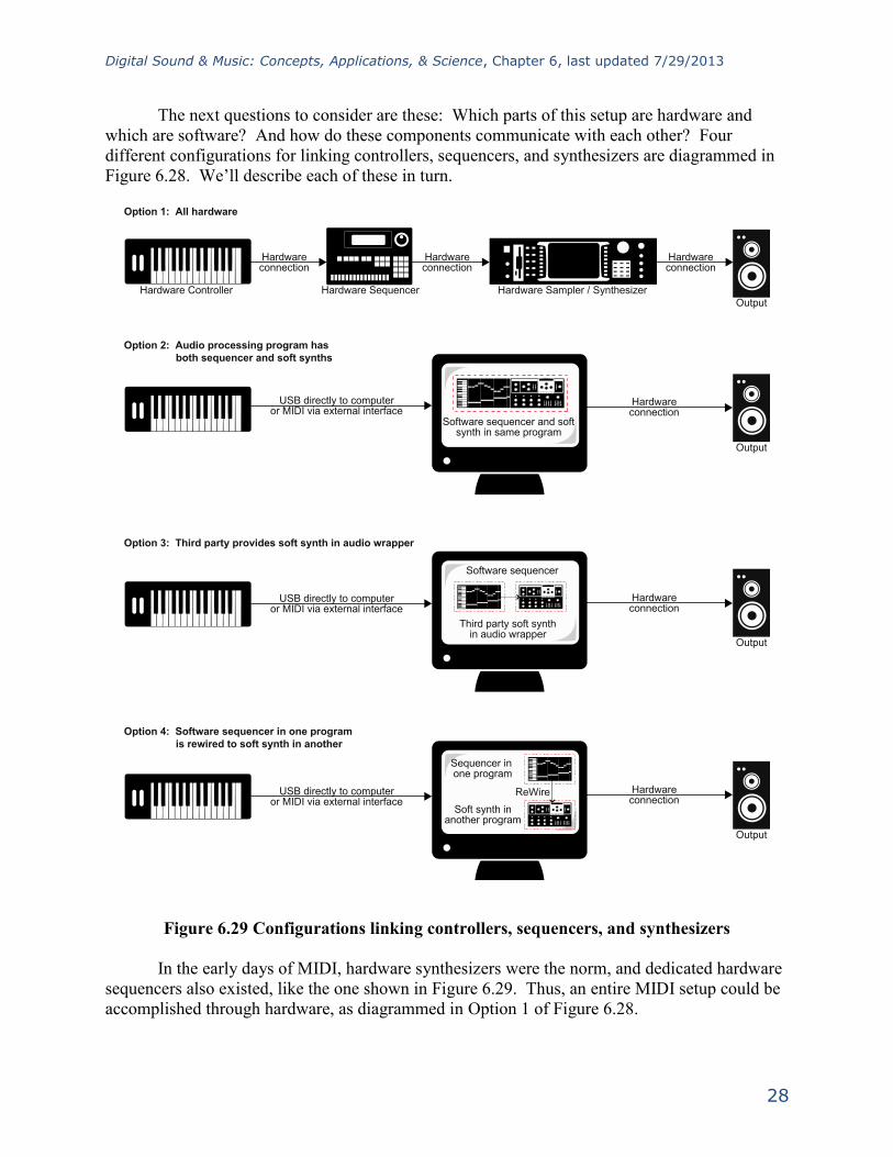
The next questions to consider are these: Which parts of this setup are hardware and
which are software? And how do these components communicate with each other? Four
different configurations for linking controllers, sequencers, and synthesizers are diagrammed in
Figure 6.28. We’ll describe each of these in turn.
Figure 6.29 Configurations linking controllers, sequencers, and synthesizers
In the early days of MIDI, hardware synthesizers were the norm, and dedicated hardware
sequencers also existed, like the one shown in Figure 6.29. Thus, an entire MIDI setup could be
accomplished through hardware, as diagrammed in Option 1 of Figure 6.28.
Option 1: All hardware
Option 2: Audio processing program has
both sequencer and soft synths
Option 3: Third party provides soft synth in audio wrapper
Option 4: Software sequencer in one program
is rewired to soft synth in another
Hardware Controller
Hardwareconnection
USB directly to computeror MIDI via external interface
Software sequencer and softsynth in same program
USB directly to computeror MIDI via external interface
USB directly to computeror MIDI via external interface
Hardwareconnection
Hardwareconnection
Hardwareconnection
Hardwareconnection
Hardwareconnection
Hardware Sequencer Hardware Sampler / Synthesizer
Output
Output
Output
Output
Third party soft synthin audio wrapper
Software sequencer
Sequencer in one program
ReWire
Soft synth inanother program
Digital Sound & Music: Concepts, Applications, & Science, Chapter 6, last updated 7/29/2013
29
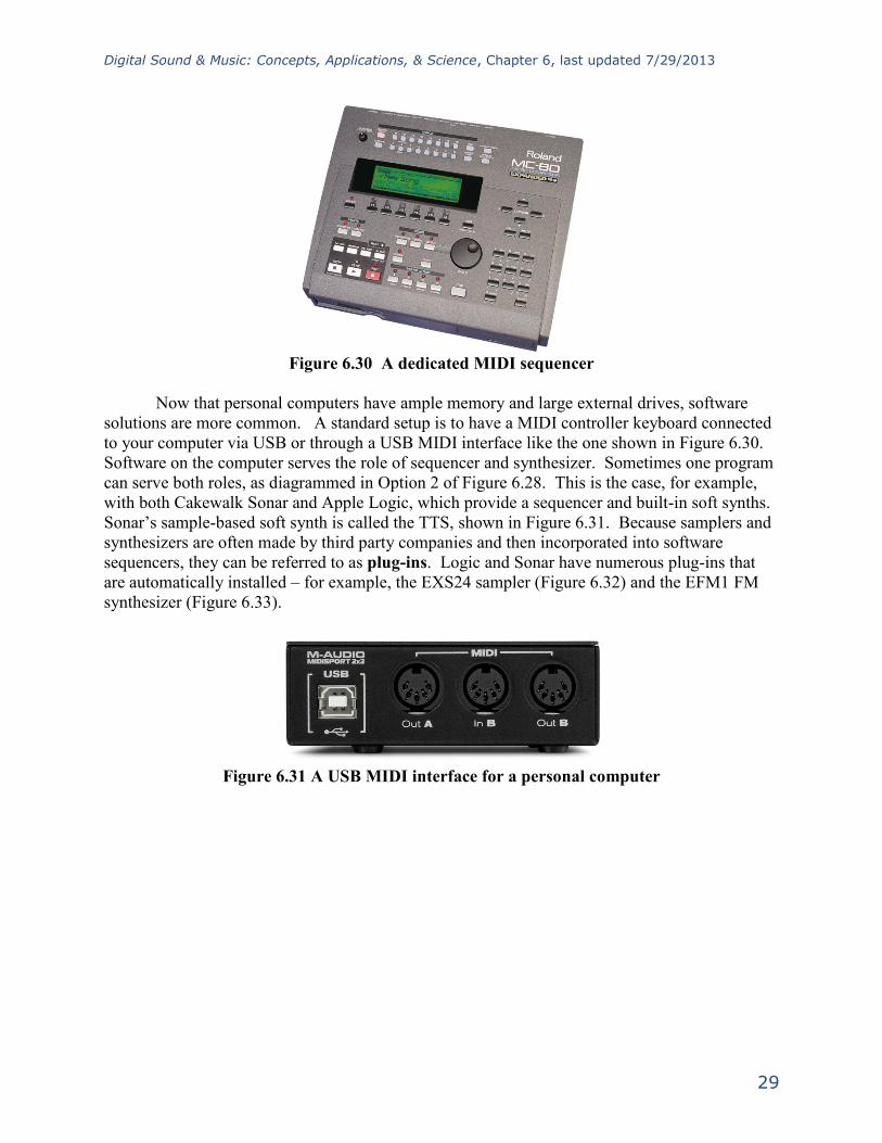
Figure 6.30 A dedicated MIDI sequencer
Now that personal computers have ample memory and large external drives, software
solutions are more common. A standard setup is to have a MIDI controller keyboard connected
to your computer via USB or through a USB MIDI interface like the one shown in Figure 6.30.
Software on the computer serves the role of sequencer and synthesizer. Sometimes one program
can serve both roles, as diagrammed in Option 2 of Figure 6.28. This is the case, for example,
with both Cakewalk Sonar and Apple Logic, which provide a sequencer and built-in soft synths.
Sonar’s sample-based soft synth is called the TTS, shown in Figure 6.31. Because samplers and
synthesizers are often made by third party companies and then incorporated into software
sequencers, they can be referred to as plug-ins. Logic and Sonar have numerous plug-ins that
are automatically installed – for example, the EXS24 sampler (Figure 6.32) and the EFM1 FM
synthesizer (Figure 6.33).
Figure 6.31 A USB MIDI interface for a personal computer

Digital Sound & Music: Concepts, Applications, & Science, Chapter 6, last updated 7/29/2013
30
Figure 6.32 TTS soft synth in Cakewalk Sonar
Figure 6.33 EXS24 sampler in Logic

Digital Sound & Music: Concepts, Applications, & Science, Chapter 6, last updated 7/29/2013
31
Figure 6.34 EFM1 synthesizer in Logic
Some third-party vendor samplers and
synthesizers are not automatically installed with
a software sequencer, but they can be added by
means of a software wrapper. The software
wrapper makes it possible for the plug-in to run
natively inside the sequencer software. This
way you can use the sequencer’s native audio
and MIDI engine and avoid the problem of
having several programs running at once and
having to save your work in multiple formats.
Typically what happens is a developer creates a
standalone soft synth like the one shown in
Figure 6.34. He can then create an Audio Unit
wrapper that allows his program to be inserted
as an Audio Unit instrument, as shown for
Logic in Figure 6.35. He can also create a VSTi
wrapper for his synthesizer that allows the
program to be inserted as a VSTi instrument in
a program like Cakewalk, an MAS wrapper for
MOTU Digital Performer, and so forth. A
setup like this is shown in Option 3 of Figure
6.28.
Aside: As you work with MIDI and
digital audio, you’ll develop a large vocabulary of abbreviations and acronyms.
In the area of plug-ins, the abbreviations relate to standardized formats that allow various software components to communicate with each other. VSTi stands for virtual studio technology instrument, created and licensed by Steinberg. This is one of the most widely
used formats. Dxi is a plug-in format based on Microsoft Direct X, and is a Windows-based format. AU, standing for audio unit, is a Mac-based format. MAS refers to plug-ins that work with Digital Performer, an audio/MIDI processing system created by the MOTU company.
RTAS (Real-Time AudioSuite) is the
protocol developed by Digidesin for Pro Tools. You need to know which formats are compatible on which platforms. You can find the most recent information through the documentation of your
software or through on-line sources.

Digital Sound & Music: Concepts, Applications, & Science, Chapter 6, last updated 7/29/2013
32
Figure 6.35 Soft synth running as a standalone application
Figure 6.36 Soft synth running in Logic through an Audio Unit instrument wrapper
An alternative to built-in synths or installed plug-ins is to have more than one program
running on your computer, each serving a different function to create the music. An example of
such a configuration would be to use Sonar or Logic as your sequencer, and then use Reason to
provide a wide array of samplers and synthesizers. This setup introduces a new question: How
do the different software programs communicate with each other?
One strategy is to create little software objects that pretend to be MIDI or audio inputs
and outputs on the computer. Instead of linking directly to input and output hardware on the
computer, you use these software objects as virtual cables. That is, the output from the MIDI

Digital Sound & Music: Concepts, Applications, & Science, Chapter 6, last updated 7/29/2013
33
sequencer program goes to the input of the software object, and the output of the software object
goes to the input of the MIDI synthesis program. The software object functions as a virtual wire
between the sequencer and synthesizer. The audio signal output by the soft synth can be routed
directly to a physical audio output on your hardware audio interface, to a separate audio
recording program, or back into the sequencer program to be stored as sampled audio data. This
configuration is diagrammed in Option 4 of Figure 6.28.
An example of this virtual wire strategy is the Rewire technology developed by
Propellerhead and used with its sampler/synthesizer program, Reason. Figure 6.36 shows how a
track in Sonar can be rewired to connect to a sampler in Reason. The track labeled “MIDI to
Reason” has the MIDI controller as its input and Reason as its output. The NN-XT sampler in
Reason translates the MIDI commands into digital audio and sends the audio back to the track
labeled “Reason to audio.” This track sends the audio output to the sound card.
Figure 6.37 Rewiring between Sonar and Reason
Other virtual wiring technologies are available. Soundflower is another program for
Mac OS X developed by Cycling ’74 that creates virtual audio wires that can be routed between
programs. CoreMIDI Virtual Ports are integrated into Apple’s CoreMIDI framework on Mac
OS X. A similar technology called MIDI Yoke (developed by a third party) works in the
Windows operating systems. Jack is an open source tool that runs on Windows, Mac OS X, and
various UNIX platforms to create virtual MIDI and audio objects.
Creating Your Own Synthesizer Sounds 6.2.2Section 6.1.8 covered the various components of a synthesizer. Now that you’ve read about the
common objects and parameters available on a synthesizer you should have an idea of what can
be done with one. So how do you know which knobs to turn and when? There’s not an easy
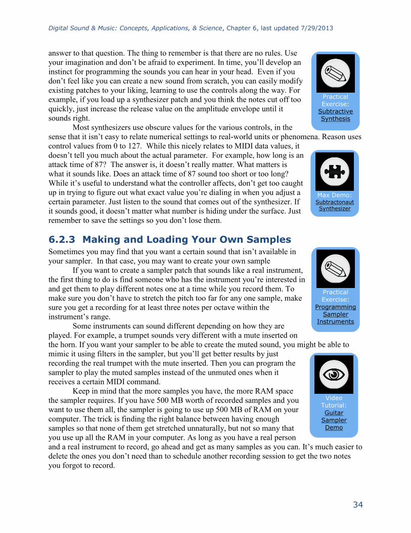
Digital Sound & Music: Concepts, Applications, & Science, Chapter 6, last updated 7/29/2013
34
answer to that question. The thing to remember is that there are no rules. Use
your imagination and don’t be afraid to experiment. In time, you’ll develop an
instinct for programming the sounds you can hear in your head. Even if you
don’t feel like you can create a new sound from scratch, you can easily modify
existing patches to your liking, learning to use the controls along the way. For
example, if you load up a synthesizer patch and you think the notes cut off too
quickly, just increase the release value on the amplitude envelope until it
sounds right.
Most synthesizers use obscure values for the various controls, in the
sense that it isn’t easy to relate numerical settings to real-world units or phenomena. Reason uses
control values from 0 to 127. While this nicely relates to MIDI data values, it
doesn’t tell you much about the actual parameter. For example, how long is an
attack time of 87? The answer is, it doesn’t really matter. What matters is
what it sounds like. Does an attack time of 87 sound too short or too long?
While it’s useful to understand what the controller affects, don’t get too caught
up in trying to figure out what exact value you’re dialing in when you adjust a
certain parameter. Just listen to the sound that comes out of the synthesizer. If
it sounds good, it doesn’t matter what number is hiding under the surface. Just
remember to save the settings so you don’t lose them. 15B
Making and Loading Your Own Samples 6.2.3Sometimes you may find that you want a certain sound that isn’t available in
your sampler. In that case, you may want to create your own sample
If you want to create a sampler patch that sounds like a real instrument,
the first thing to do is find someone who has the instrument you’re interested in
and get them to play different notes one at a time while you record them. To
make sure you don’t have to stretch the pitch too far for any one sample, make
sure you get a recording for at least three notes per octave within the
instrument’s range.
Some instruments can sound different depending on how they are
played. For example, a trumpet sounds very different with a mute inserted on
the horn. If you want your sampler to be able to create the muted sound, you might be able to
mimic it using filters in the sampler, but you’ll get better results by just
recording the real trumpet with the mute inserted. Then you can program the
sampler to play the muted samples instead of the unmuted ones when it
receives a certain MIDI command.
Keep in mind that the more samples you have, the more RAM space
the sampler requires. If you have 500 MB worth of recorded samples and you
want to use them all, the sampler is going to use up 500 MB of RAM on your
computer. The trick is finding the right balance between having enough
samples so that none of them get stretched unnaturally, but not so many that
you use up all the RAM in your computer. As long as you have a real person
and a real instrument to record, go ahead and get as many samples as you can. It’s much easier to
delete the ones you don’t need than to schedule another recording session to get the two notes
you forgot to record.
Practical
Exercise:
Programming Sampler
Instruments
Video
Tutorial:
Guitar
Sampler Demo
Practical Exercise:
Subtractive Synthesis
Max Demo: Subtractonaut Synthesizer
http://csweb.cs.wfu.edu/~burg/CCLI/Tutorials/Worksheets/Chapter6/Programming_Sampler_Instruments.zip
http://csweb.cs.wfu.edu/~burg/CCLI/Tutorials/Worksheets/Chapter6/Programming_Sampler_Instruments.zip
Digital Sound & Music: Concepts, Applications, & Science, Chapter 6, last updated 7/29/2013
35
Once you have all your samples recorded, you need to edit them and add all the metadata
required by the sampler. In order for the sampler to do what it needs to do with the audio files,
the files need to be in an uncompressed file format. Usually this is WAV or AIF format. Some
samplers have a limit on the sampling rate they can work with. Make sure you convert the
samples to the rate required by the sampler before you try to use them.
The first bit of metadata you need to add to each sample is a loop start and loop end
marker. Because you’re working with prerecorded sounds, the sound doesn't necessarily keep
playing just because you’re still holding the key down on the keyboard. You could just record
your samples so they hold on for a long time, but that would use up an
unnecessary amount of RAM. Instead, you can tell the sampler to play the file
from the beginning and stop playing the file when the key on the keyboard is
released. If the key is still down when the sampler reaches the end of the file,
the sampler can start playing a small portion of the sample over and over in an
endless loop until the note is released. The challenge here is finding a portion of
the sample that loops naturally without any clicks or other swells in amplitude
or harmonics.
Figure 6.37 shows a loop defined in a sample editing program. On the
left side of the screen you can see the overall waveform of the sample, in this
case a violin. In the time ruler above the waveform you can see a green bar labeled Sustaining
Loop. This is the portion of the sample that is looped. On the right side of the screen you can see
a close up view of the loop point. The left half of the wave is the end of the sample, and the right
part of the wave is the start of the loop point. The trick here is to line up the loop points so the
two parts intersect with the zero amplitude cross point. This way you avoid any clicks or pops
that might be introduced when the sampler starts looping the playback.
Video
Tutorial: Recorder Sampler Demo

Digital Sound & Music: Concepts, Applications, & Science, Chapter 6, last updated 7/29/2013
36
Figure 6.38 Editing sample loop points
In some sample editors you can also add other metadata that saves you programming time
later. For WAV and AIF files, you can add information about the root pitch of the sample and the
range of notes this sample should cover. You can also add information about the loop behavior.
For example, do you want the sample to continue to loop during the release of the amplitude
envelope, or do you want it to start playing through to the end of the file? You could set the
sample not to loop at all and instead play as a “one shot” sample. This means the sample ignores
Note Off events and play the sample from beginning to end every time. Some samplers can read
that metadata and do some pre-programming for you on the sampler when you load the sample.

Digital Sound & Music: Concepts, Applications, & Science, Chapter 6, last updated 7/29/2013
37
Figure 6.39 Adding sample metadata such as root pitch and loop type
Once the samples are ready, you can load them into the sampler. If you weren’t able to
add the metadata about root key and loop type, you’ll have to add that manually into the sampler
for each sample. You’ll also need to decide which notes trigger each sample and which velocities
each sample responds to. This process of assigning root keys and key ranges to all your samples
is a time consuming but essential process. Figure 6.39 shows a list of sample WAV files loaded
in a software sampler. In the figure we have the sample “PianoC43.wav” selected. You can see
in the center of the screen the span of keys that have been assigned to that sample. Along the
bottom row of the screen you can see the root key, loop, and velocity assignments for that
sample.
Figure 6.40 Loading and assigning samples in a software sampler

Digital Sound & Music: Concepts, Applications, & Science, Chapter 6, last updated 7/29/2013
38
Once you have all your samples loaded and assigned, each sample can be passed through
a filter and amplifier which can in turn be modulated using envelopes, LFO, and MIDI controller
commands. Most samplers let you group samples together into zones or keygroups allowing you
to apply a single set of filters, envelopes, etc. This feature can save a lot of time in programming.
Imagine programming all of those settings on each of 100 samples without losing track of how
far you are in the process. Figure 6.40 shows all the common synthesizer objects being applied to
the “PianoC43.wav” sample.
Figure 6.41 Synthesizer functions that can be applied to samples once they have been
loaded and assigned
Data Flow and Performance Issues in Audio/MIDI 6.2.4Recording
Combined audio/MIDI recording can place high demands on a system, requiring a fast CPU and
hard drive, an appropriate choice of audio driver, and a careful setting of the audio buffer size.
These components affect your ability to record, process, and play sound, particularly in real time.
Digital Sound & Music: Concepts, Applications, & Science, Chapter 6, last updated 7/29/2013
39
In Chapter 5, we introduced the subject of latency in digital audio systems. The problem
of latency is compounded when MIDI data is added to the mix. A common frustration in MIDI
recording sessions is that there can be an audible difference between the moment when you press
a key on a MIDI controller keyboard and the moment when you hear the sound coming out of the
headphones or monitors. In this case, the latency is the result of your buffer size. The MIDI
signal generated by the key press must be transformed into digital audio by a synthesizer or
sampler, and the digital data is then placed in the output buffer. This sound is not heard until the
buffer is filled up. When the buffer is full, it undergoes ADC and is set sent to the headphones or
monitors. Playback latency results when the buffer is too large. As discussed in Chapter 5, you
can reduce the playback latency by using a low latency audio driver like ASIO or reducing the
buffer size if this option is available in your driver. However, if you make the buffer size too
low, you’ll have breaks in the sound when the CPU cannot keep up with the number of times it
has to empty the buffer.
Another potential bottleneck in digital audio playback is the hard drive. Fast hard drives
are a must when working with digital audio, and it is also important to use a dedicated hard drive
for your audio files. If you’re storing your audio files on the same hard drive as your operating
system, you’ll need a larger playback buffer to accommodate all the times the hard drive is busy
delivering system data instead of your audio. If you get a second hard drive and use it only for
audio files, you can usually get away with a much smaller playback buffer, thereby reducing the
playback latency.
When you use software instruments, there are other system resources besides the hard
drive that also become a factor to consider. Software samplers require a lot of system RAM
because all the audio samples have to be loaded completely in RAM in order for them to be
instantly accessible. On the other hand, software synthesizers that generate the sound
dynamically can be particularly hard on the CPU. The CPU has to mathematically create the
audio stream in real time, which is a more computationally intense process than simply playing
an audio stream that already exists. Synthesizers with multiple oscillators can be particularly
problematic. Some programs let you offload individual audio or instrument tracks to another
CPU. This could be a networked computer running a processing node program or some sort of
dedicated processing hardware connected to the host computer. If you’re having problems with
playback dropouts due to CPU overload and you can’t add more CPU power, another strategy is
to render the instrument audio signal to an audio file that is played back instead of generated live
(often called “freezing” a track). However, this effectively disables the MIDI signal and the
software instrument so if you need to make any changes to the rendered track, you need to go
back to the MIDI data and re-render the audio.
Non-Musical Applications for MIDI 6.2.5
MIDI Show Control 6.2.5.1MIDI is not limited to use for digital music. There have been many additions to the MIDI
specification to allow MIDI to be used in other areas. One addition is the MIDI Show Control
Specification. MIDI Show Control (MSC) is used in live entertainment to control sound,
lighting, projection, and other automated features in theatre, theme parks, concerts, and more.
MSC is a subset of the MIDI Systems Exclusive (SysEx) status byte. MIDI SysEx
commands are typically specific to each manufacturer of MIDI devices. Each manufacturer gets
Digital Sound & Music: Concepts, Applications, & Science, Chapter 6, last updated 7/29/2013
40
a SysEx ID number. MSC has a SysEx sub-ID number of 0x02. The syntax, in hexadecimal, for
a MSC message is:
F0 7F <device_ID> 02 <command_format> <command> <data> F7
F0 is the status byte indicating the start of a SysEx message.
7F indicates the use of a SysEx sub-ID. This is technically a manufacturer ID that has
been reserved to indicate extensions to the MIDI specification.
<device_ID> can be any number between 0x00 and 0x7F indicating the device ID of the
thing you want to control. These device ID numbers have to be set on the receiving end
as well so each device knows which messages to respond to and which messages to
ignore. 0x7F is a universal device ID. All devices respond to this ID regardless of their
individual ID numbers.
02 is the sub-ID number for MIDI Show Control. This tells the receiving device that the
bytes that follow are MIDI Show Control syntax as opposed to MIDI Machine Control,
MIDI Time Code, or other commands.
<command_format> is a number indicating the type of device being controlled. For
example, 0x01 indicates a lighting device, 0x40 indicates a projection device, and 0x60
indicates a pyrotechnics device. A complete list of command format numbers can be
found in the MIDI Show Control 1.1 specification.
<command> is a number indicating the type of command being sent. For example, 0x01 is
“GO”, 0x02 is “STOP”, 0x03 is “RESUME”, 0x0A is “RESET”.
<data> represents a variable number of data bytes that are required for the type of
command being sent. A “GO” command might need some data bytes to indicate the cue
number that needs to be executed from a list of cues on the device. If no cue number is
specified, the device simply executes the next cue in the list. Two data bytes (0x00, 0x00)
are still needed in this case as delimiters for the cue number syntax. Some MSC devices
are able to interpret the message without these delimiters, but they're technically required
in the MSC specification.
F7 is the End of Systems Exclusive byte indicating the end of the message.
Most lighting consoles, projection systems, and computer sound playback systems used in
live entertainment are able to generate and respond to MSC messages. Typically, you don't have
to create the commands manually in hex. You have a graphical interface that lets you choose the
command you're want from a list of menus. Figure 6.41 shows some MSC FIRE commands for a
lighting console generated as part of a list of sound cues. In this case, the sound effect of a
firecracker is synchronized with the flash of a strobe light using MSC.

Digital Sound & Music: Concepts, Applications, & Science, Chapter 6, last updated 7/29/2013
41
Figure 6.42 A list of sound and MIDI Show Control cues in a sound playback system for
live entertainment
MIDI Relays and Footswitches 6.2.5.2You may not always have a device that knows how to respond to MIDI commands. For example,
although there is a MIDI Show Control command format for motorized scenery, the motor that
moves a unit on or off the stage doesn’t understand MIDI commands. However, it does
understand a switch. There are many options available for MIDI controlled relays that respond to
a MIDI command by making or breaking an electrical contact closure. This makes it possible for
you to connect the wires for the control switch of a motor to the relay output, and then when you
send the appropriate MIDI command to the relay, it closes the connection and the motor starts
turning.
Another possibility is that you may want to use MIDI commands without a traditional
MIDI controller. For example, maybe you want a sound effect to play each time a door is opened

Digital Sound & Music: Concepts, Applications, & Science, Chapter 6, last updated 7/29/2013
42
or closed. Using a MIDI footswitch device, you could wire up a magnetic door sensor to the
footswitch input and have a MIDI command sent to the computer each time the door is opened or
closed. The computer could then be programmed to respond by playing a sound file. Figure 6.42
shows an example of a MIDI relay device.
Figure 6.43 A MIDI controllable relay
MIDI Time Code 6.2.5.3MIDI sequencers, audio editors, and audio playback systems often need to synchronize their
timeline with other systems. Synchronization could be needed for working with sound for video,
lighting systems in live performance, and even automated theme part attractions. The world of
filmmaking has been dealing with synchronization issues for decades, and the Society of Motion
Picture and Television Engineers (SMPTE) has developed a standard format for a time code that
can be used to keep video and audio in sync. Typically this is accomplished using an audio signal
called Linear Time Code that has the synchronization data encoded in SMPTE format. The
format is Hours:Minutes:Seconds:Frames. The number of frames per second varies, but the
standard allows for 24, 25, 29.97 (also known as 30-Drop), and 30 frames per second.
MIDI Time Code (MTC) uses this same time code format, but instead of being encoded
into an analog audio signal, the time information is transmitted in digital format via MIDI. A full
MIDI Time Code message has the following syntax:
F0 7F <device_ID> <sub-ID 1> <sub-ID 2> <hr> <mn> <sc> <fr> F7
F0 is the status byte indicating the start of a SysEx message.
7F indicates the use of a SysEx sub-ID. This is technically a manufacturer ID that has
been reserved to indicate extensions to the MIDI specification.
<device_ID> can be any number between 0x00 and 0x7F indicating the device ID of the
thing you want to control. These device ID numbers have to be set on the receiving end
as well so each device knows which messages to respond to and which messages to
ignore. 0x7F is a universal device ID. All devices respond to this ID regardless of their
individual ID numbers.

Digital Sound & Music: Concepts, Applications, & Science, Chapter 6, last updated 7/29/2013
43
<sub-ID 1> is the sub-ID number for MIDI Time Code. This tells the receiving device
that the bytes that follow are MIDI Time Code syntax as opposed to MIDI Machine
Control, MIDI Show Control, or other commands. There are a few different MIDI Time
Code sub ID numbers. 01 is used for full SMPTE messages and for SMPTE user bits
messages. 04 is used for a MIDI Cueing message that includes a SMPTE time along with
values for markers such as Punch In/Out and Start/Stop points. 05 is used for real-time
cuing messages. These messages have all the marker values but use the quarter-frame
format for the time code.
<sub-ID 2> is a number used to define the type of message within the sub-ID 1 families.
For example, there are two types of Full Messages that use 01 for sub-ID 1. A value of 01
for sub-ID 2 in a Full Message would indicate a Full Time Code Message whereas 02
would indicate a User Bits Message.
<hr> is a byte that carries both the hours value as well as the frame rate. Since there are
only 24 hours in a day, the hours value can be encoded using the five least significant
bits, while the next two greater significant bits are used for the frame rate. With those two
bits you can indicate four different frame rates (24, 25, 29.97, 30). As this is a data byte,
the most significant bit stays at 0.
<mn> represents the minutes value 0059.
<sc> represents the seconds value 0059.
<fr> represents the frame value 0029.
F7 is the End of Systems Exclusive byte indicating the end of the message.
For example, to send a message that sets the current timeline location of every device in the
system to 01:30:35:20 in 30 frames/second format, the hexadecimal message would be:
F0 7F 7F 01 01 61 1E 23 14 F7
Once the full message has been transmitted, the time code is sent in quarter-frame format.
Quarter-frame messages are much smaller than full messages. This is less demanding of the
system since only two bytes rather than ten bytes have to be parsed at a time. Quarter frame
messages use the 0xF1 status byte and one data byte with the high nibble indicating the message
type and the low nibble indicating the value of the given time field. There are eight message
types, two for each time field. Each field is separated into a least significant nibble and a most
significant nibble:
0 = Frame count LS
1 = Frame count MS
2 = Seconds count LS
3 = Seconds count MS
4 = Minutes count LS
5 = Minutes count MS
6 = Hours count LS
7 = Hours count MS and SMPTE frame rate
Digital Sound & Music: Concepts, Applications, & Science, Chapter 6, last updated 7/29/2013
44
As the name indicates, quarter frame messages are transmitted in increments of four
messages per frame. Messages are transmitted in the order listed above. Consequently, the entire
SMPTE time is completed every two frames. Let’s break down the same 01:30:35:20 time value
into quarter frame messages in hexadecimal. This time value would be broken up into eight
messages:
F1 04 (Frame LS)
F1 11 (Frame MS)
F1 23 (Seconds LS)
F1 32 (Seconds MS)
F1 4E (Minutes LS)
F1 51 (Minutes MS)
F1 61 (Hours LS)
F1 76 (Hours MS and Frame Rate)
When synchronizing systems with MIDI Time Code, one device needs to be the master
time code generator and all other devices need to be configured to follow the time code from this
master clock. Figure 6.43 shows Logic Pro configured to synchronize to an incoming MIDI Time
Code signal. If you have a mix of devices in your system that follow LTC or MTC, you can also
put a dedicated time code device in your system that collects the time code signal in LTC or
MTC format and then relay that time code to all the devices in your system in the various
formats required, as shown in Figure 6.44.

Digital Sound & Music: Concepts, Applications, & Science, Chapter 6, last updated 7/29/2013
45
Figure 6.44 MIDI Time Code synchronization for Logic Pro
Figure 6.45 A dedicated SMPTE synchronization device capable of distributing Linear
Time Code and MIDI Time Code
MIDI Machine Control 6.2.5.4Another subset of the MIDI specification is a set of commands that can control
the transport system of various recording and playback systems. Transport
controls are things like play, stop, rewind, record, etc. This command set is
called MIDI Machine Control. The specification is quite comprehensive and
includes options for SMPTE time code values, as well as confirmation response
messages from the devices being controlled. A simple MMC message has the
following syntax:
F0 7F <device_ID> 06 <command> F7
F0 is the status byte indicating the start of a SysEx message.
7F indicates the use of a SysEx sub-ID. This is technically a manufacturer ID that has
been reserved to indicate extensions to the MIDI specification.
<device_ID> can be any number between 0x00 and 0x7F indicating the device ID of the
thing you want to control. These device ID numbers have to be set on the receiving end
as well so each device knows which messages to respond to and which messages to
Max Demo:
MTC MMC

Digital Sound & Music: Concepts, Applications, & Science, Chapter 6, last updated 7/29/2013
46
ignore. 0x7F is a universal device ID. All devices respond to this ID regardless of their
individual ID numbers.
06 is the sub-ID number for MIDI Machine Control. This tells the receiving device that
the bytes that follow are MIDI Machine Control syntax as opposed to MIDI Show
Control, MIDI Time Code, or other commands.
<command> can be a set of bytes as small as one byte and can include several bytes
communicating various commands in great detail. A simple play (0x02) or stop (0x01)
command only requires a single data byte.
F7 is the End of Systems Exclusive byte indicating the end of the message.
A MMC command for PLAY would look like this:
F0 7F 7F 06 02 F7
MIDI Machine Control was really a necessity when most studio recording systems were
made up of several different magnetic tape-based systems or dedicated hard disc recorders. In
these situations, a single transport control would make sure all the devices were doing the
same thing. In today’s software-based systems, MIDI Machine Control is primarily used with
MIDI control surfaces, like the one shown in Figure 6.45, that connect to a computer so you
can control the transport of your DAW software without having to manipulate a mouse.
Figure 6.46 A dedicated MIDI Machine Control device
6.3 Science, Mathematics, and Algorithms
MIDI SMF Files 6.3.1If you'd like to dig into the MIDI specification more deeply – perhaps writing a program that can
either generate a MIDI file in the correct format or interpret one and turn it into digital audio –
you need to know more about how the files are formatted.
Standard MIDI Files (SMF), with the .mid or .smf suffix, encode MIDI data in a
prescribed format for the header, timing information, and events. Format 0 files are for single

Digital Sound & Music: Concepts, Applications, & Science, Chapter 6, last updated 7/29/2013
47
tracks, Format1 files are for multiple tracks, and Format 2 files are for multiple tracks where a
separate song performance can be represented. (Format 2 is not widely used.) SMF files are
platform-independent, interpretable on PCs, MAC, and Linux machines.
Blocks of information in SMF files are called chunks. The first chunk is the header
chunk, followed by one or more data chunks. The header and data chunks begin with four
bytes (a four-character string) identifying the type of chunk they are. The header chunk then has
four bytes giving the length of the remaining fields of the chunk (which is always 6 for the
header), two bytes telling the format (MIDI 0, 1, or 2), two bytes telling the number of tracks,
and two bytes with information about how timing is handled.
Data are stored in track chunks. A track chunk also begins with four bytes telling the
type of chunk followed by four bytes telling how much data is in the chunk. The data then
follow. The bytes which constitute the data are track events: either regular MIDI events like
Note On; meta-events like changes of tempo, key, or time signature; or sys-ex events. The
events begin with a timestamp telling when they are to happen. Then the rest of the data are
MIDI events with the format described in Section 1. The structure of an SMF file is illustrated in
Figure 6.47.
Figure 6.47 SMF file structure
MIDI event timestamps tell the change in time between the previous event and the current
one, using the tick-per-beat, frame rate in frames/s, and tick/frame defined in the header. The
timestamp itself is given in a variable-length field. To accomplish this, the first bit of each byte
in the timestamp indicates how many bytes are to follow in the timestamp. If the bit is a 0, then

Digital Sound & Music: Concepts, Applications, & Science, Chapter 6, last updated 7/29/2013
48
the value in the following seven bits of the byte make up the full value of the timestamp. If the
bit is a 1, then the next byte is also to be considered part of the timestamp value. This ultimately
saves space. It would be wasteful to dedicate four bytes to the timestamp just to take care of the
few cases where there is a long pause between one MIDI event and the next one.
An important consideration in writing or reading SMF files is the issue of whether bytes
are stored in little-endian or big-endian format. In big-endian format, the most significant byte
is stored first in a sequence of bytes that make up one value. In little-endian, the least
significant byte is stored first. SMF files store bytes in big-endian format. If you're writing an
SMF-interpreting program, you need to check the endian-ness of the processor and operating
system on which you'll be running the program. A PC/Windows combination is generally little-
endian, so a program running on that platform has to swap the byte-order when determining the
value of a multiple-byte timestamp.
More details about SMF files can be found at www.midi.org. To see the full MIDI
specification, you have to order and pay for the documentation. (Messick 1998) is a good source
to help you write a C++ program that reads and interprets SMF files.
Shaping Synthesizer Parameters with Envelopes and 6.3.2LFOs
Let's make a sharp turn now from MIDI specifications to the mathematics and algorithms under
the hood of synthesizers.
In Section 6.1.8.7, envelopes were discussed as a way of modifying the parameters of
some synthesizer function – for example, the cutoff frequency of a low or high pass filter or the
amplitude of a waveform. The mathematics of envelopes is easy to understand. The graph of
the envelope shows time on the horizontal axis and a "multiplier" or coefficient on the vertical
axis. The parameter is question is simply multiplied by the coefficient over time.
Envelopes can be generated by simple or complex functions. The envelope could be a
simple sinusoidal, triangle, square, or sawtooth function that causes the parameter to go up and
down in this regular pattern. In such cases, the envelope is called an oscillator. The term low-
frequency oscillator (LFO) is used in synthesizers because the rate at which the parameter is
caused to change is low compared to audible frequencies.
An ADSR envelope has a shape like the one shown in Figure 6.25. Such an envelope can
be defined by the attack, decay, sustain, and release points, between which straight (or evenly
curved) lines are drawn. Again, the values in the graph represent multipliers to be applied to a
chosen parameter.
The exercise associated with this section invites you to modulate one or more of the
parameters of an audio signal with an LFO and also with an ASDR envelope that you define
yourself.
Type of Synthesis 6.3.3
Table-Lookup Oscillators and Wavetable 6.3.3.1Synthesis
We have seen how single-frequency sound waves are easily generated by means of sinusoidal
functions. In our example exercises, we've done this through computation, evaluating sine
functions over time. In contrast, table-lookup oscillators generate waveforms by means of a set

Digital Sound & Music: Concepts, Applications, & Science, Chapter 6, last updated 7/29/2013
49
of look-up wavetables stored in contiguous memory locations. Each wavetable contains a list of
sample values constituting one cycle of a sinusoidal wave, as illustrated in Figure 6.48. Multiple
wavetables are stored so that waveforms of a wide range of frequencies can be generated.
1 0.0490676743274180
2 0.098017140329561
3 0.146730474455362
…
128 -2.449293598294706e-16
wavetable
Figure 6.48 A wavetable in a table-lookup oscillator
With a table-lookup oscillator, a waveform is created by advancing a pointer
through a wavetable, reading the values, cycling back to the beginning of the table as
necessary, and outputting the sound wave accordingly.
With a table of N samples representing one cycle of a waveform and an
assumed sampling rate of r samples/s, you can generate a fundamental frequency of r/N
Hz simply by reading the values out of the table at the sampling rate. This entails
stepping through the indexes of the consecutive memory locations of the table. The
wavetable in Figure 6.48 corresponds to a fundamental frequency of
.
Harmonics of the fundamental frequency of the wavetable can be created by
skipping values or inserting extra values in between those in the table. For example,
you can output a waveform with twice the frequency of the fundamental by reading out every
other value in the table. You can output a waveform with ½ the frequency of the fundamental by
reading each value twice, or by inserting values in between those in the table by interpolation.
The phase of the waveform can be varied by starting at an offset from the beginning of
the wavetable. To start at a phase offset of radians, you would start reading at index
. For
example, to start at an offset of in the wavetable of Figure 6.48, you would start at index
.
To generate a waveform that is not a harmonic of the fundamental frequency, it's
necessary to add an increment to the consecutive indexes that are read out from the table. This
increment i depends on the desired frequency f, the table length N, and the sampling rate r,
defined by
. For example, to generate a waveform with frequency 750 Hz using the
wavetable of Figure 6.48 and assuming a sampling rate of 48000 Hz, you would need an
increment of
. We've chosen an example where the increment is an integer,
which is good because the indexes into the table have to be integers.
MATLAB Exercise:
Creating and Using a
Wavetable in MATLAB

Digital Sound & Music: Concepts, Applications, & Science, Chapter 6, last updated 7/29/2013
50
What if you wanted a frequency of 390 Hz? Then the increment would be
, which is not an integer. In cases where the increment is not an integer, interpolation must
be used. For example, if you want to go an increment of 1.04 from index 1, that would take you
to index 2.04. Assuming that our wavetable is called table, you want a value equal to
[ ] [ ] [ ] . This is a rough way to do interpolation. Cubic
spline interpolation can also be used as a better way of shaping the curve of the waveform. The
exercise associated with this section suggests that you experiment with table-lookup oscillators
in MATLAB.
An extension of the use of table-lookup oscillators is
wavetable synthesis. Wavetable synthesis was introduced in digital
synthesizers in the 1970s by Wolfgang Palm in Germany. This was
the era when the transition was being made from the analog to the
digital realm. Wavetable synthesis uses multiple wavetables,
combining them with additive synthesis and crossfading and
shaping them with modulators, filters, and amplitude envelopes.
The wavetables don't necessarily have to represent simple
sinusoidals but can be more complex waveforms. Wavetable
synthesis was innovative in the 1970s in allowing for the creation of
sounds not realizable with by solely analog means. This synthesis method has now evolved to the
NWave-Waldorf synthesizer for the iPad.
Additive Synthesis 6.3.3.2In Chapter 2, we introduced the concept of frequency components of complex waves. This is
one of the most fundamental concepts in audio processing, dating back to the groundbreaking
work of Jean-Baptiste Fourier in the early 1800s. Fourier was able to prove that any periodic
waveform is composed of an infinite sum of single-frequency waveforms of varying frequencies
and amplitudes. The single-frequency waveforms that are summed to make the more complex
one are called the frequency components.
The implications of Fourier’s discovery are far reaching. It means that, theoretically, we
can build whatever complex sounds we want just by adding sine waves. This is the basis of
additive synthesis. We demonstrated how it worked in Chapter 2, illustrated by the production
of square, sawtooth, and triangle waveforms. Additive synthesis of each of these waveforms
begins with a sine wave of some fundamental frequency, f. As you recall, a square wave is
constructed from an infinite sum of odd-numbered harmonics of f of diminishing amplitude, as in
A sawtooth waveform can be constructed from an infinite sum of all harmonics of f of
diminishing amplitude, as in
(
)
A triangle waveform can be constructed from an infinite sum of odd-numbered harmonics of f
that diminish in amplitude and vary in their sign, as in
Aside: The term "wavetable" is sometimes used to refer a memory
bank of samples used by sound cards for MIDI sound generation. This can be
misleading terminology, as wavetable synthesis is a different thing entirely.
Digital Sound & Music: Concepts, Applications, & Science, Chapter 6, last updated 7/29/2013
51
(
)
These basic waveforms turn out to be very important in subtractive synthesis, as they serve as a
starting point from which other more complex sounds can be created.
To be able to create a sound by additive synthesis, you need to know the frequency
components to add together. It's usually difficult to get the sound you want by adding
waveforms from the ground up. In turns out that subtractive synthesis is often an easier way to
proceed.
Subtractive Synthesis 6.3.3.3The first synthesizers, including the Moog and Buchla’s Music Box, were analog synthesizers
that made distinctive electronic sounds different from what is produced by traditional
instruments. This was part of the fascination that listeners had for them. They did this by
subtractive synthesis, a process that begins with a basic sound and then selectively removes
frequency components. The first digital synthesizers imitated their analog precursors. Thus,
when people speak of “analog synthesizers” today, they often mean digital subtractive
synthesizers. The Subtractor Polyphonic Synthesizer shown in Figure 6.19 is an example of one
of these.
The development of subtractive synthesis arose from an analysis of musical instruments
and the way they create their sound, the human voice being among those instruments. Such
sounds can be divided into two components: a source of excitation and a resonator. For a violin,
the source is the bow being drawn across the string, and the resonator is the body of the violin.
For the human voice, the source results from air movement and muscle contractions of the vocal
chords, and the resonator is the mouth. In a subtractive synthesizer, the source could be a pulse,
sawtooth, or triangle wave or random noise of different colors (colors corresponding to how the
noise is spread out over the frequency spectrum). Frequently, preset patches are provided, which
are basic waveforms with certain settings like amplitude envelopes already applied (another
usage of the term patch). Filters are provided that allow you to remove selected frequency
components. For example, you could start with a sawtooth wave and filter out some of the
higher harmonic frequencies, creating something that sounds fairly similar to a stringed
instrument. An amplitude envelope could be applied also to shape the attack, decay, sustain, and
release of the sound.
The exercise suggests that you experiment with subtractive synthesis in C++ by
beginning with a waveform, subtracting some of its frequency components, and applying an
envelope.
Amplitude Modulation (AM) 6.3.3.4Amplitude, phase, and frequency modulation are three types of modulation that can be applied to
synthesize sounds in a digital synthesizer. We explain the mathematical operations below. In
Section 0, we defined modulation as the process of changing the shape of a waveform over time.
Modulation has long been used in analog telecommunication systems as a way to transmit a
signal on a fixed frequency channel. The frequency on which a television or radio station is

Digital Sound & Music: Concepts, Applications, & Science, Chapter 6, last updated 7/29/2013
52
broadcast is referred to as the carrier signal and the message "written on" the carrier is called
the modulator signal. The message can be encoded on the carrier signal in one of three ways:
AM (amplitude modulation), PM (phase modulation), or FM (frequency modulation).
Amplitude modulation (AM) is commonly used in radio transmissions. It entails
sending a message by modulating the amplitude of a carrier signal with a modulator signal.
In the realm of digital sound as created by synthesizers, AM can be used to generate a
digital audio signal of N samples by application of the following equation:
( )
Equation 6.1 Amplitude modulation for digital synthesis
The process is expressed algorithmically in Algorithm 6.8. The algorithm shows that the
AM synthesis equation must be applied to generate each of the samples for .
algorithm amplitude_modulation
/*
Input:
f_c, the frequency of the carrier signal
f_m, the frequency of a low frequency modulator signal
N, the number of samples you want to create
r, the sampling rate
A, to adjust the amplitude of the
Output:
y, an array of audio samples where the carrier has been amplitude
modulated by the modulator */
{
for (n = 1 to N)
y[n] = sin(2*pi*f_c*n/r) * (1.0 + A*cos(2*pi*f_m*n/r));
}
Algorithm 6.1 Amplitude modulation for digital synthesis
Algorithm 6.1can be executed at the MATLAB command line with the statements below,
generating the graphs is Figure 6.49. Because MATLAB executes the statements as vector
operations, a loop is not required. (Alternatively, a MATLAB program could be written using a
loop.) For simplicity, we'll assume in what follows.
N = 44100;
r = 44100;
n = [1:N];
f_m = 10;
f_c = 440;
m = cos(2*pi*f_m*n/r);
c = sin(2*pi*f_c*n/r);
figure;

Digital Sound & Music: Concepts, Applications, & Science, Chapter 6, last updated 7/29/2013
53
AM = c.*(1.0 + m);
plot(m(1:10000));
axis([0 10000 -2 2]);
figure;
plot(c(1:10000));
axis([0 10000 -2 2]);
figure;
plot(AM(1:10000));
axis([0 10000 -2 2]);
wavplay(c, 44100);
wavplay(m, 44100);
wavplay(AM, 44100);
This yields the following graphs:
440 Hz carrier wave
10 Hz modulator wave
result of amplitude modulation
Figure 6.49 Amplitude modulation using two sinusoidals
If you listen to the result, you'll see that amplitude modulation creates a kind of tremolo effect.
The same process can be accomplished with more complex waveforms. HornsE04.wav
is a 132,300-sample audio clip of horns playing, at a sampling rate of 44,100 Hz. Below, we
shape it with a 440 Hz cosine wave (Figure 6.50).
N = 132300;
r = 44100;
c = wavread('HornsE04.wav');
n = [1:N];
m = sin(2*pi*10*n/r);
m = transpose(m);
AM2 = c .* (1.0 + m);
figure;
plot(c);
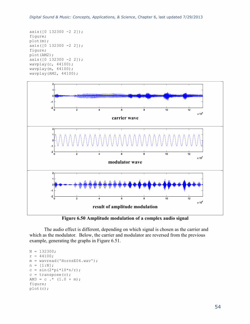
Digital Sound & Music: Concepts, Applications, & Science, Chapter 6, last updated 7/29/2013
54
axis([0 132300 -2 2]);
figure;
plot(m);
axis([0 132300 -2 2]);
figure;
plot(AM2);
axis([0 132300 -2 2]);
wavplay(c, 44100);
wavplay(m, 44100);
wavplay(AM2, 44100);
carrier wave
modulator wave
result of amplitude modulation
Figure 6.50 Amplitude modulation of a complex audio signal
The audio effect is different, depending on which signal is chosen as the carrier and
which as the modulator. Below, the carrier and modulator are reversed from the previous
example, generating the graphs in Figure 6.51.
N = 132300;
r = 44100;
m = wavread('HornsE04.wav');
n = [1:N];
c = sin(2*pi*10*n/r);
c = transpose(c);
AM3 = c .* (1.0 + m);
figure;
plot(c);
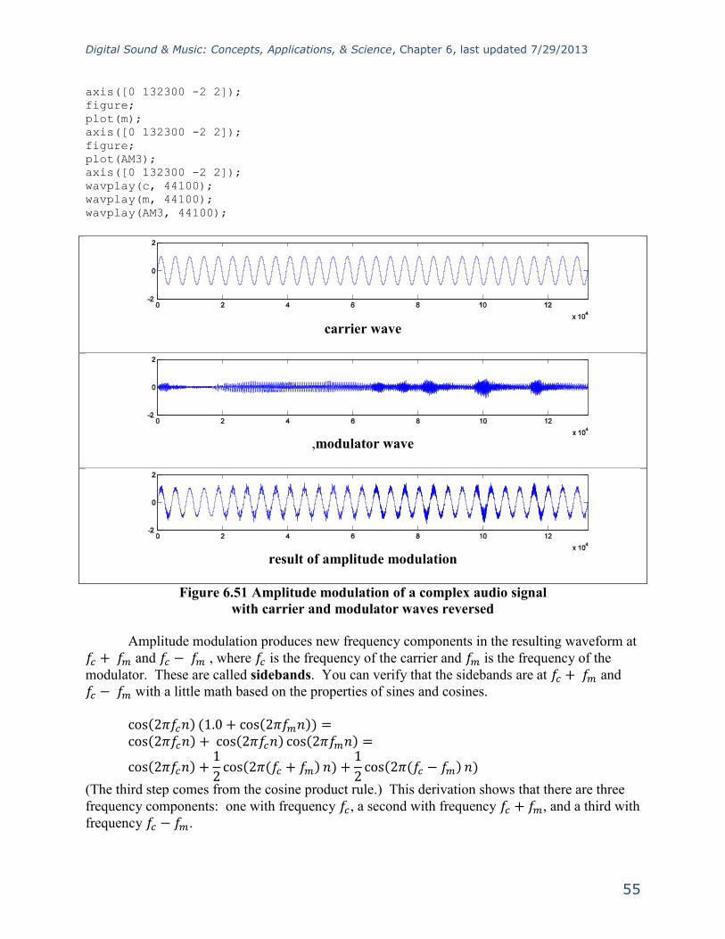
Digital Sound & Music: Concepts, Applications, & Science, Chapter 6, last updated 7/29/2013
55
axis([0 132300 -2 2]);
figure;
plot(m);
axis([0 132300 -2 2]);
figure;
plot(AM3);
axis([0 132300 -2 2]);
wavplay(c, 44100);
wavplay(m, 44100);
wavplay(AM3, 44100);
carrier wave
,modulator wave
result of amplitude modulation
Figure 6.51 Amplitude modulation of a complex audio signal
with carrier and modulator waves reversed
Amplitude modulation produces new frequency components in the resulting waveform at
and , where is the frequency of the carrier and is the frequency of the
modulator. These are called sidebands. You can verify that the sidebands are at and
with a little math based on the properties of sines and cosines.
(The third step comes from the cosine product rule.) This derivation shows that there are three
frequency components: one with frequency , a second with frequency , and a third with
frequency .
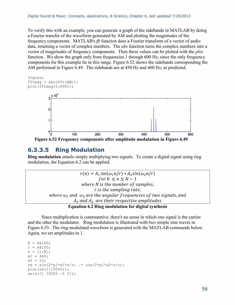
Digital Sound & Music: Concepts, Applications, & Science, Chapter 6, last updated 7/29/2013
56
To verify this with an example, you can generate a graph of the sidebands in MATLAB by doing
a Fourier transfer of the waveform generated by AM and plotting the magnitudes of the
frequency components. MATLAB's fft function does a Fourier transform of a vector of audio
data, returning a vector of complex numbers. The abs function turns the complex numbers into a
vector of magnitudes of frequency components. Then these values can be plotted with the plot
function. We show the graph only from frequencies 1 through 600 Hz, since the only frequency
components for this example lie in this range. Figure 6.52 shows the sidebands corresponding the
AM performed in Figure 6.49. The sidebands are at 450 Hz and 460 Hz, as predicted.
figure;
fftmag = abs(fft(AM));
plot(fftmag(1:600));
Figure 6.52 Frequency components after amplitude modulation in Figure 6.49
Ring Modulation 6.3.3.5Ring modulation entails simply multiplying two signals. To create a digital signal using ring
modulation, the Equation 6.2 can be applied.
,
Equation 6.2 Ring modulation for digital synthesis
Since multiplication is commutative, there's no sense in which one signal is the carrier
and the other the modulator. Ring modulation is illustrated with two simple sine waves in
Figure 6.53. The ring modulated waveform is generated with the MATLAB commands below.
Again, we set amplitudes to 1.
N = 44100;
r = 44100;
n = [1:N];
w1 = 440;
w2 = 10;
rm = sin(2*pi*w1*n/r) .* cos(2*pi*w2*n/r);
plot(rm(1:10000));
axis([1 10000 -2 2]);

Digital Sound & Music: Concepts, Applications, & Science, Chapter 6, last updated 7/29/2013
57
result of ring modulation
Figure 6.53 Ring modulation using two sinusoidals
Phase Modulation (PM) 6.3.3.6Even more interesting audio effects can be created with phase (PM) and frequency modulation
(FM). We're all familiar with FM radio, which is based on sending a signal by frequency
modulation. Phase modulation is not used extensively in radio transmissions because it can be
ambiguous to interpret at the receiving end, but it turns out to be fairly easy to implement PM in
digital synthesizers. Some hardware-based synthesizers that are commonly referred to as FM
actually use PM synthesis internally – the Yamaha DX series, for example.
Recall that the general equation for a cosine waveform is where f is the
frequency and is the phase. Phase modulation involves changing the phase over time.
Equation 6.3 uses phase modulation to generate a digital signal.
( )
Equation 6.3 Phase modulation for digital synthesis
Phase modulation is demonstrated in MATLAB with the following statements:
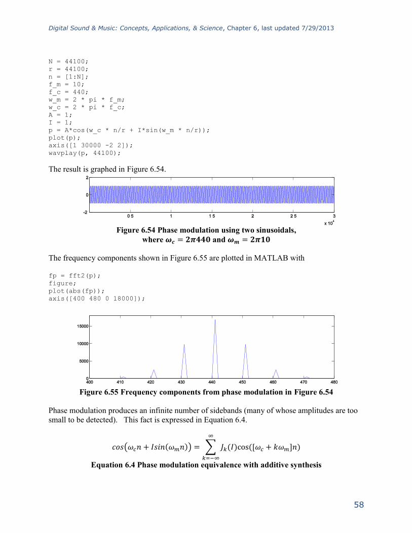
Digital Sound & Music: Concepts, Applications, & Science, Chapter 6, last updated 7/29/2013
58
N = 44100;
r = 44100;
n = [1:N];
f_m = 10;
f_c = 440;
w_m = 2 * pi * f_m;
w_c = 2 * pi * f_c;
A = 1;
I = 1;
p = A*cos(w_c * n/r + I*sin(w_m * n/r));
plot(p);
axis([1 30000 -2 2]);
wavplay(p, 44100);
The result is graphed in Figure 6.54.
Figure 6.54 Phase modulation using two sinusoidals,
where and
The frequency components shown in Figure 6.55 are plotted in MATLAB with
fp = fft2(p);
figure;
plot(abs(fp));
axis([400 480 0 18000]);
Figure 6.55 Frequency components from phase modulation in Figure 6.54
Phase modulation produces an infinite number of sidebands (many of whose amplitudes are too
small to be detected). This fact is expressed in Equation 6.4.
( ) ∑ [
]
Equation 6.4 Phase modulation equivalence with additive synthesis

Digital Sound & Music: Concepts, Applications, & Science, Chapter 6, last updated 7/29/2013
59
gives the amplitude of the frequency component for each kth
component in the
phase-modulated signal. These scaling functions are called Bessel functions of the first
kind. It's beyond the scope of the book to define these functions further. You can experiment for
yourself to see that the frequency components have amplitudes that depend on I. If you listen to
the sounds created, you'll find that the timbres of the sounds can also be caused to change over
time by changing I. The frequencies of the components, on the other hand, depend on the ratio
of . You can try varying the MATLAB commands above to experience the wide variety
of sounds that can be created with phase modulation. You should also consider the possibilities
of applying additive or subtractive synthesis to multiple phase-modulated waveforms.
Frequency Modulation (FM) 6.3.3.7We have seen in the previous section that phase modulation can be applied to the digital
synthesis of a wide variety of waveforms. Frequency modulation is equally versatile and
frequently used in digital synthesizers. Frequency modulation is defined recursively as follows:
and
(
(
)),
, and
,
,
,
Equation 6.5 Frequency modulation for digital synthesis
Frequency modulation can yield results identical to phase modulation,
depending on how inputs parameters are handled in the implementation. A
difference between phase and frequency modulation is the perspective from which
the modulation is handled. Obviously, the former is shaping a waveform by
modulating the phase, while the latter is modulating the frequency. In frequency
modulation, the change in the frequency can be handled by a parameter d, an
absolute change in carrier signal frequency, which is defined by . The
input parameters , , , , , and
yield the graphs shown in Figure 6.56 and Figure 6.57. We suggest that
you try to replicate these results by writing a MATLAB program based on
Equation 6.5 defining frequency modulation.
Figure 6.56 Frequency modulation using two sinusoidals,
MATLAB Exercise:
Frequency Modulation for Digital
Synthesis in MATLAB
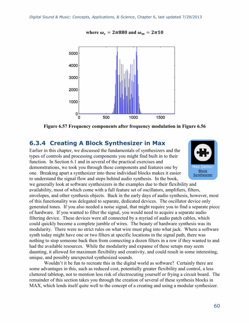
Digital Sound & Music: Concepts, Applications, & Science, Chapter 6, last updated 7/29/2013
60
where and
Figure 6.57 Frequency components after frequency modulation in Figure 6.56
Creating A Block Synthesizer in Max 6.3.4Earlier in this chapter, we discussed the fundamentals of synthesizers and the
types of controls and processing components you might find built in to their
function. In Section 6.1 and in several of the practical exercises and
demonstrations, we took you through these components and features one by
one. Breaking apart a synthesizer into these individual blocks makes it easier
to understand the signal flow and steps behind audio synthesis. In the book,
we generally look at software synthesizers in the examples due to their flexibility and
availability, most of which come with a full feature set of oscillators, amplifiers, filters,
envelopes, and other synthesis objects. Back in the early days of audio synthesis, however, most
of this functionality was delegated to separate, dedicated devices. The oscillator device only
generated tones. If you also needed a noise signal, that might require you to find a separate piece
of hardware. If you wanted to filter the signal, you would need to acquire a separate audio
filtering device. These devices were all connected by a myriad of audio patch cables, which
could quickly become a complete jumble of wires. The beauty of hardware synthesis was its
modularity. There were no strict rules on what wire must plug into what jack. Where a software
synth today might have one or two filters at specific locations in the signal path, there was
nothing to stop someone back then from connecting a dozen filters in a row if they wanted to and
had the available resources. While the modularity and expanse of these setups may seem
daunting, it allowed for maximum flexibility and creativity, and could result in some interesting,
unique, and possibly unexpected synthesized sounds.
Wouldn’t it be fun to recreate this in the digital world as software? Certainly there are
some advantages in this, such as reduced cost, potentially greater flexibility and control, a less
cluttered tabletop, not to mention less risk of electrocuting yourself or frying a circuit board. The
remainder of this section takes you through the creation of several of these synthesis blocks in
MAX, which lends itself quite well to the concept of a creating and using a modular synthesizer.
Max Demo:
Block
Synthesizer

Digital Sound & Music: Concepts, Applications, & Science, Chapter 6, last updated 7/29/2013
61
At the end of this example, we’ll see how we can then combine and connect these blocks in any
imaginable configuration to possibly create some never-before-heard sounds.
It is assumed that you're proficient in the basics of MAX. If you're not familiar with an
object we use or discuss, please refer to the MAX help and reference files for that object (Help >
Open [ObjectName] Help in the file menu, or Right-click > Open [ObjectName] Help). Every
object in MAX has a help file that explains and demonstrates how the object works.
Additionally, if you hover the mouse over an inlet or outlet of an object, MAX often shows you a
tooltip with information on its format or use. We also try to include helpful comments and hints
within the solution itself.
At this point in the chapter, you should be familiar with a good number of these synthesis
blocks and how they are utilized. We’ll look at how you might create an audio oscillator, an
amplification stage, and an envelope block to control some of our synth parameters. Before we
get into the guts of the synth blocks, let’s take a moment to think about how we might want to
use these blocks together and consider some of the features of MAX that lend themselves to this
modular approach.
It would be ideal to have a single window where you could add blocks and arrange and
connect them in any way you want. The blocks themselves would need to have input and
outputs for audio and control values. The blocks should have the relevant and necessary controls
(knobs, sliders, etc.) and displays. We also don't necessarily need to see the inner workings of
the completed blocks, and because screen space is at a premium, the blocks should be as compact
and simply packaged as possible. From a programming point of view, the blocks should be
easily copied and pasted, and if we had to change the internal components of one type of block it
would be nice if the change reflected across all the other blocks of that type. In this way, if we
wanted, say, to add another waveform type to our oscillator blocks later on, and we had already
created and connected dozens of oscillator blocks, we wouldn’t have to go through and
reprogram each one individually.
There is an object in MAX called the bpatcher. It is similar in a sense to a typical
subpatcher object, in that it provides a means to create multiple elements and a complex
functionality inside of one single object. However, where the subpatcher physically contains the
additional objects within it, the bpatcher essentially allows you to embed an entire other patcher
file inside your current one. It also provides a “window” into the patcher file itself, showing a
customizable area of the embedded patcher contents. Additionally, like the subpatcher, the
bpatcher allows for connection to and from custom inlets and outlets in the patcher file. Using
the bpatcher object, we're able to create each synth block in its own separate patcher file. We
can configure the customizable viewing window to maximize display potential while keeping
screen real estate to a minimum. Creating another block is as simple as duplicating the one
bpatcher object (no multiple objects to deal with), and as the bpatcher links to the one external
file, updating the block file updates all of the instances in our main synthesizer file. To tell a
bpatcher which file to link, you open the bpatcher Inspector window (Object > Inspector in the
file menu, or select the object and Right-click > Inspector) and click the Choose button on the
Patcher File line to browse for the patcher file, as shown in Figure 6.46.
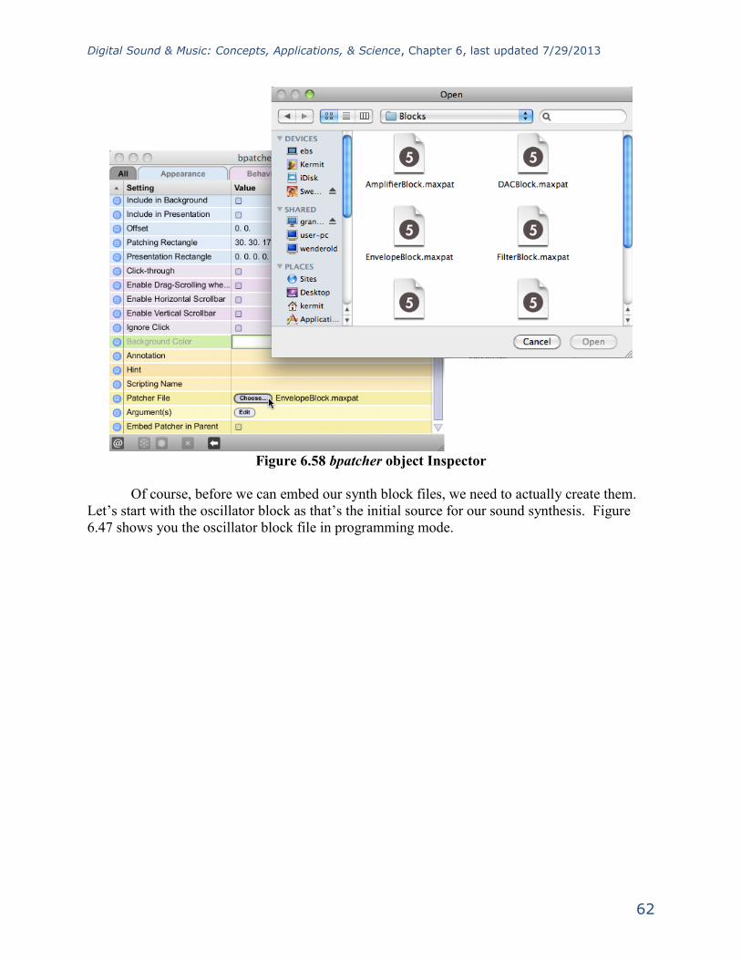
Digital Sound & Music: Concepts, Applications, & Science, Chapter 6, last updated 7/29/2013
62
Figure 6.58 bpatcher object Inspector
Of course, before we can embed our synth block files, we need to actually create them.
Let’s start with the oscillator block as that’s the initial source for our sound synthesis. Figure
6.47 shows you the oscillator block file in programming mode.
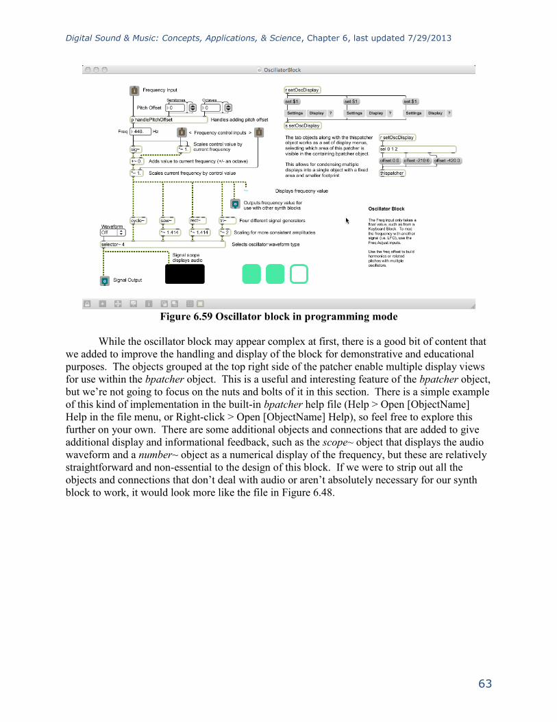
Digital Sound & Music: Concepts, Applications, & Science, Chapter 6, last updated 7/29/2013
63
Figure 6.59 Oscillator block in programming mode
While the oscillator block may appear complex at first, there is a good bit of content that
we added to improve the handling and display of the block for demonstrative and educational
purposes. The objects grouped at the top right side of the patcher enable multiple display views
for use within the bpatcher object. This is a useful and interesting feature of the bpatcher object,
but we’re not going to focus on the nuts and bolts of it in this section. There is a simple example
of this kind of implementation in the built-in bpatcher help file (Help > Open [ObjectName]
Help in the file menu, or Right-click > Open [ObjectName] Help), so feel free to explore this
further on your own. There are some additional objects and connections that are added to give
additional display and informational feedback, such as the scope~ object that displays the audio
waveform and a number~ object as a numerical display of the frequency, but these are relatively
straightforward and non-essential to the design of this block. If we were to strip out all the
objects and connections that don’t deal with audio or aren’t absolutely necessary for our synth
block to work, it would look more like the file in Figure 6.48.

Digital Sound & Music: Concepts, Applications, & Science, Chapter 6, last updated 7/29/2013
64
Figure 6.60 Oscillator block stripped down
In its most basic functionality, the oscillator block simply generates an audio signal of
some kind. In this case, we chose to provide several different options for the audio signal,
including an object for generating basic sine waves (cycle~), sawtooth waves (saw~), square
waves (rect~) and triangle waves (tri~). Each of these objects takes a number in to its leftmost
inlet to set its frequency. The selector~ object is used to select between multiple signals, and the
desired signal is passed through based on the waveform selected in the connected user interface
dropdown menu (umenu). The inlets and outlets may seem strange when used in a standalone
patcher file, and at this stage they aren’t really useful. However, when the file is linked into the
bpatcher object, these inlets and outlets appear on the bpatcher and allow you access to these
signals and control values in the main synth patcher.
While this module alone would enable you to begin synthesizing simple sounds, one of
the purposes of the modular synthesizer blocks is to be able to wire them together to control each
other in interesting ways. In this respect, we may want to consider ways to control or manipulate
our oscillator block. The primary parameter in the case of the oscillator is the oscillator
frequency, so we should incorporate some control elements for it. Perhaps we would want to
increase or decrease the oscillator frequency, or even scale it by an external factor. Consider the
way some of the software or hardware synths previously discussed in this chapter have
manipulated the oscillator frequency. Looking back at the programming mode for this block,
you may recall seeing several inlets labeled “frequency control” and some additional connected
objects. A close view of these can be seen in Figure 6.49.

Digital Sound & Music: Concepts, Applications, & Science, Chapter 6, last updated 7/29/2013
65
Figure 6.61 Oscillator block frequency control inputs
These control inputs are attached to several arithmetic objects, including addition and
multiplication. The “~” following the mathematical operator simply means this version of the
object is used for processing signal rate (audio) values. This is the sole purpose of the sig~
object also seen here; it takes the static numerical value of the frequency (shown at 440 Hz) and
outputs it as a signal rate value, meaning it is constantly streaming its output. In the case of these
two control inputs, we set one of them up as an additive control, and the other a multiplicative
control. The inlet on the left is the additive control. It adds to the oscillator frequency an
amount equal to some portion of the current oscillator frequency value. For example, if for the
frequency value shown it receives a control value of 1, it adds 440 Hz to the oscillator frequency.
If it receives a control value of 0.5, it adds 220 Hz to the oscillator frequency. If it receives a
control value of 0, it adds nothing to the oscillator frequency, resulting in no change.
At this point we should take a step back and ask ourselves, “What kind of control values
should we be expecting?” There is really no one answer to this, but as the designers of these
synth blocks we should perhaps establish a convention that is meaningful across all of our
different synthesizer elements. For our purposes, a floating-point range between 0.0 and 1.0
seems simple and manageable. Of course, we can’t stop someone from connecting a control
value outside of this range to our block if they really wanted. That’s just what makes modular
synthesis so fun.
Going back to the second control input (multiplicative), you can see that it scales the
output of the oscillator directly by this control value. If it receives a control value of 0, the
oscillator’s frequency is 0 and it outputs silence. If it receives a control value of 1, the signal is
multiplied by 1, resulting in no change. Notice that the multiplication object has been set to a
default value of 1 so that the initial oscillator without any control input behaves normally. The
addition object has been initialized for that behavior as well. It is also very important to include
the “.” with these initial values, as that tells the object to expect a floating-point value rather than
an integer (default). Without the decimal, the object may round or truncate the floating-point
value to the nearest integer, resulting in our case to a control value of either 0 or 1, which would
be rather limiting.
Let’s now take a look at what goes into an amplification block. The amplification block
is simply used to control the amplitude, or level, of the synthesized audio. Figure 6.50 shows
you our amplifier block file in programming mode. There isn’t much need to strip down the
non-essentials from this block, as there’s just not much to it.

Digital Sound & Music: Concepts, Applications, & Science, Chapter 6, last updated 7/29/2013
66
Figure 6.62 Amplifier block in programming mode
Tracing the audio signal path straight down the left side of the patcher, you can see that
there are two stages of multiplication, which essentially is amplification in the digital realm. The
first stage of amplification is controlled by a level slider and a mute toggle switch. These
interface objects allow the overall amplification to be set graphically by the user. The second
stage of amplification is set by an external control value. Again this is another good fit for the
standard range we decided on of 0.0 to 1.0. A control value of 0 causes the signal amplitude to
be scaled to 0, outputting silence. A control value of 1 results in no change in amplification. On
the other hand, could you think of a reason we might want to increase the amplitude of the
signal, and input a control value greater than 1.0? Perhaps a future synth block may have good
reason to do this. Now that we have these available control inputs, we should start thinking of
how we might actually control these blocks, such as with an envelope.
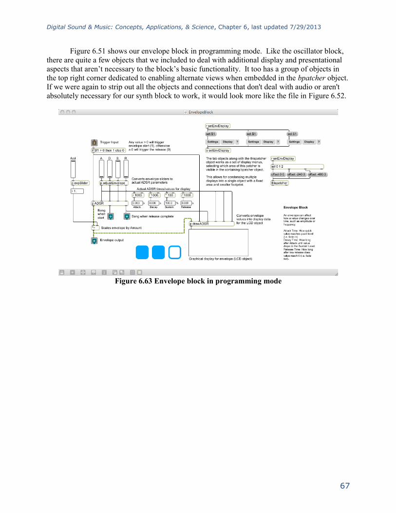
Digital Sound & Music: Concepts, Applications, & Science, Chapter 6, last updated 7/29/2013
67
Figure 6.51 shows our envelope block in programming mode. Like the oscillator block,
there are quite a few objects that we included to deal with additional display and presentational
aspects that aren’t necessary to the block’s basic functionality. It too has a group of objects in
the top right corner dedicated to enabling alternate views when embedded in the bpatcher object.
If we were again to strip out all the objects and connections that don't deal with audio or aren't
absolutely necessary for our synth block to work, it would look more like the file in Figure 6.52.
Figure 6.63 Envelope block in programming mode

Digital Sound & Music: Concepts, Applications, & Science, Chapter 6, last updated 7/29/2013
68
Figure 6.64 Envelope block stripped down
While it incorporates signal rate objects, the envelope doesn’t actually involve the audio
signal. Its output is purely used for control. Then again, it's possible for the user to connect the
envelope block output to the audio signal path, but it probably won’t sound very good if it even
makes a sound at all. Let’s start with the inlet at the top. In order for an envelope to function
properly, it has to know when to start and when to stop. Typically it starts when someone
triggers a note, such as by playing a key on a keyboard, and releases when the key is let go.
Thinking back to MIDI and how MIDI keyboards work, we know that when a key is pressed, it
sends a Note On command accompanied by a velocity value of between 1 and 127. When the
key is released, it often sends a Note On command with a velocity value of zero. In our case, we
don’t really care what the value is between 1 and 127; we need to start the envelope regardless of
how hard the key is pressed.
This velocity value lends itself to being a good way to tell when to trigger and release an
envelope. It would be useful to condition the input to give us only the two cases we care about:
start and release. There are certainly multiple ways to implement this in MAX, but a simple
if…then object is an easy way to check this logic using one object. The if…then object checks if

Digital Sound & Music: Concepts, Applications, & Science, Chapter 6, last updated 7/29/2013
69
the value at inlet 1 ($f1) is greater than 0 (as is the case for 1 to 127), and if so it outputs the
value 1. Otherwise, (if the inlet value is less than or equal to 0) it outputs 0. Since there are no
negative velocity values, we’ve just lumped them into the release outcome to cover our bases.
Now our input value results in a 1 or a 0 relating to a start or release envelope trigger.
As is often the case, it just so happens that MAX has a built in adsr~ object that generates
a standard ADSR envelope. We opted to create our own custom ADSR subpatcher. However,
its purpose and inlets/outlets are essentially identical, and it’s meant to be easily interchangeable
with the adsr~ object. You can find out more about our custom ADSR subpatcher and the
reason for its existence in the MAX Demo “ADSR Envelopes” back in section 6.1.8.5.1. For the
moment, we’ll refer to it as the standard adsr~ object.
Now, it just so happens that the adsr~ object’s first inlet triggers the envelope start when
it sees any non-zero number, and it triggers the release when it receives a 0. Our input is thus
already primed to be plugged straight into this object. It may also seem that our conditioning is
now somewhat moot, since any typical velocity value, being a positive number, triggers the
envelope start of the adsr~ object just as well as the number 1. It is however still important to
consider that perhaps the user may (for creative reasons) connect a different type of control value
to the envelope trigger input, other than note velocity. The conditioning if…then object thereby
ensures a more widely successful operation with potentially unexpected input formats.
The adsr~ object also takes four other values as input. These are, as you might imagine,
the attack time, decay time, sustain value, and release time. For simple controls, we’ve provided
the user with four sliders to manipulate these parameters. In between the sliders and the adsr~
inlets, we need to condition the slider values to relate to usable ADSR values. The subpatcher
adjustEnvelope does just that, and its contents can be seen in Figure 6.53. The four slider values
(default 0 to 127) are converted to time values of appropriate scale, and in the case of sustain a
factor ranging from 0.0 to 1.0. The expSlider subpatchers as seen in earlier MAX demos give
the sliders an exponential curve, allowing for greater precision at lower values.
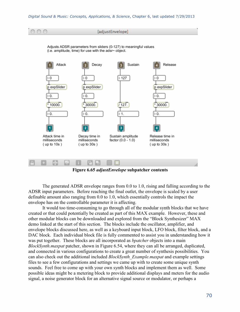
Digital Sound & Music: Concepts, Applications, & Science, Chapter 6, last updated 7/29/2013
70
Figure 6.65 adjustEnvelope subpatcher contents
The generated ADSR envelope ranges from 0.0 to 1.0, rising and falling according to the
ADSR input parameters. Before reaching the final outlet, the envelope is scaled by a user
definable amount also ranging from 0.0 to 1.0, which essentially controls the impact the
envelope has on the controllable parameter it is affecting.
It would too time-consuming to go through all of the modular synth blocks that we have
created or that could potentially be created as part of this MAX example. However, these and
other modular blocks can be downloaded and explored from the “Block Synthesizer” MAX
demo linked at the start of this section. The blocks include the oscillator, amplifier, and
envelope blocks discussed here, as well as a keyboard input block, LFO block, filter block, and a
DAC block. Each individual block file is fully commented to assist you in understanding how it
was put together. These blocks are all incorporated as bpatcher objects into a main
BlockSynth.maxpat patcher, shown in Figure 6.54, where they can all be arranged, duplicated,
and connected in various configurations to create a great number of synthesis possibilities. You
can also check out the additional included BlockSynth_Example.maxpat and example settings
files to see a few configurations and settings we came up with to create some unique synth
sounds. Feel free to come up with your own synth blocks and implement them as well. Some
possible ideas might be a metering block to provide additional displays and meters for the audio
signal, a noise generator block for an alternative signal source or modulator, or perhaps a
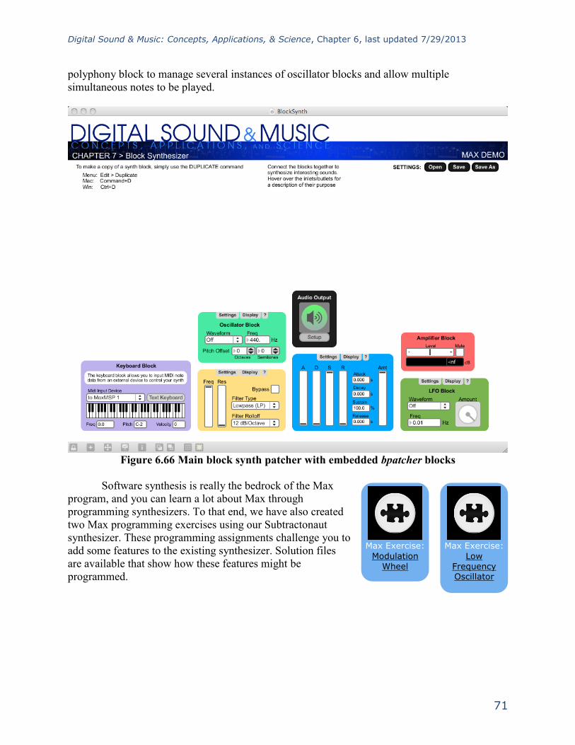
Digital Sound & Music: Concepts, Applications, & Science, Chapter 6, last updated 7/29/2013
71
polyphony block to manage several instances of oscillator blocks and allow multiple
simultaneous notes to be played.
Figure 6.66 Main block synth patcher with embedded bpatcher blocks
Software synthesis is really the bedrock of the Max
program, and you can learn a lot about Max through
programming synthesizers. To that end, we have also created
two Max programming exercises using our Subtractonaut
synthesizer. These programming assignments challenge you to
add some features to the existing synthesizer. Solution files
are available that show how these features might be
programmed.
Max Exercise:
Modulation Wheel
Max Exercise:
Low Frequency Oscillator
Digital Sound & Music: Concepts, Applications, & Science, Chapter 6, last updated 7/29/2013
72
6.4 References In addition to references cited in previous chapters:
Boulanger, Richard, and Victor Lazzarini, eds. The Audio Programming Book. Cambridge,
MA: The MIT Press, 2011.
Huntington, John. Control Systems for Live Entertainment. Boston: Focal Press, 1994.
Messick, Paul. Maximum MIDI: Music Applications in C++. Greenwich, CT: Manning
Publications, 1998.
Schaeffer, Pierre. A la Recherche d’une Musique Concrète. Paris: Editions du Seuil, 1952.


![Chapter 10 The Disklavier & MIDI€¦ · 02/01/2010 · MIDI Drum Machine or Sequencer MIDI OUT MIDI CABLE or S. 55 English Chapter 10: The Disklavier & MIDI 6 Press [+/YES] to set](https://static.fdocuments.in/doc/165x107/603e37739ee5d3297807dffc/chapter-10-the-disklavier-midi-02012010-midi-drum-machine-or-sequencer.jpg)


![USB MIDI/LTC Widget MIDI LTC... · USB MIDI/LTC Widget 1.783 [45.28] 7.808 [198.33] Timecode- Single Linear Input Connection- USB-B (1) MIDI-Input-Supports- MIDI MIDI Show Control](https://static.fdocuments.in/doc/165x107/5f8814d97ac2ab28ba5b1540/usb-midiltc-widget-midi-ltc-usb-midiltc-widget-1783-4528-7808-19833.jpg)