CHAPTER 6MESB 374

System Modeling and Analysis

Hydraulic (Fluid) Systems

Hydraulic (Fluid) Systems• Basic Modeling Elements

– Resistance

– Capacitance

– Inertance

– Pressure and Flow Sources

• Interconnection Relationships– Compatibility Law

– Continuity Law

• Derive Input/Output Models

The analogy between the hydraulic system and the electrical system will be used often. Just as in electrical systems, the flow rate (current) is defined to be the time rate of change (derivative) of volume (charge):

The pressure, p, used in this chapter is the absolute pressure. You need to be careful in determining whether the pressure is the absolute pressure or gauge pressure, p*. Gauge pressure is the difference between the absolute pressure and the atmospheric pressure, i.e.

Variables• q : volumetric flow rate [m3/sec] ( )

p p patmospheric*

dq V V

dt

current

voltage• p : pressure [N/m2] ( )

charge• V : volume [m3] ( )

• Fluid ResistanceDescribes any physical element with the characteristic that the pressure drop,p ,across the element is proportional to the flow rate, q.

– Orifices, valves, nozzles and friction in pipes can be modeled as fluid resistors.

Basic Modeling Elements

p p p p R q

qR

pR

p

1 2 12

12

1 1

Ex: The flow that goes through an orifice or a valve and the turbulent flow that goes through a pipe is related to the pressure drop by

Find the effective flow resistance of the element at certain operating point ( ).

q p, 12

q k p 12

q

p12

12 12

122

12,

1

2

2 2

q p

d q k

R d p p

p qR

k k

qR

+ p p1 p2+ p

R

p1 p2

qq

p12

Basic Modeling Elements

• Fluid CapacitanceDescribes any physical element with the characteristic that the rate of change in pressure, p, in the element is proportional to the difference between the input flow rate, qIN , and the output flow rate, qOUT .

– Hydraulic cylinder chambers, tanks, and accumulators are examples of fluid capacitors.

gh

Cd

dtp p C p q qC ref Cr IN OUT

pCr

qIN

pref

C

pC qOUT

CqIN - qOUT

+ pCr

Ex: Consider an open tank with a constant cross-sectional area, A:

qIN qOUT

pC

h

pr

C

IN OUT

Cr

p

q q

p

C

d dVolum Ah Ah

dt dt

rgh p Crp gh

gh IN OUT

Cr

q q Ah A

p ggh

Ex:Will the effective capacitance change if in the previous open tank example, a load mass M is floating on top of the tank?

Ex: Calculate the equivalent fluid capacitance for a hydraulic chamber with only an inlet port.

Recall the bulk modulus () of a fluid is defined by:

Fluid Capacitance Examples

qIN

pr

C

pC

chamber volume V

Cr

C

V dq p

dt

qIN qOUT

pC

h

pr

M

Cr

Cr

dpdtdp

V VdVdV

dt

C

IN OUT

Cr

p

q q

p

C

d dVolum Ah Ah

dt dt

rMggh p A Cr

Mgp gh A

gh IN OUT

Cr

q q Ah A

p ggh

Basic Modeling Elements• Fluid Inertance (Inductance)

Describes any physical element with the characteristic that the pressure drop, p , across the element is proportional to the rate of change (derivative) of the flow rate, q.

– Long pipes are examples of fluid inertances.

1 1F Ap

p p p p Id

dtq I q 12 1 2( )

Ex: Consider a section of pipe with cross-sectional area A and length L, filled with fluid whose density is :

Start with force balance: F = ma Iq

p1 p2+ p

q

+ p

I

p1 p2

L

q

p1 p2+ p

A

IL

A

2 2F Ap1 1F Ap

1 2 1 2 12F F F A p p Ap m LA

12

mFa

dv d qAp AL AL

dt dt A

12

I

L dqp

A dt

• Pressure Source (Pump)– An ideal pressure source of a

hydraulic system is capable of maintaining the desired pressure, regardless of the flow required for what it is driving.

• Flow Source (Pump)– An ideal flow source is capable

of delivering the desired flow rate, regardless of the pressure required to drive the load.

Basic Modeling Elements

pS +p1 p2

pS q

p p p pS21 2 1

p1 p2

qS q

q qS

Voltage Source

Current Source

Interconnection Laws• Compatibility Law

– The sum of the pressure drops around a loop must be zero.

– Similar to the Kirchhoff’s voltage law.

• Continuity Law– The algebraic sum of the flow rates

at any junction in the loop is zero.

– This is the consequence of the conservation of mass.

– Similar to the Kirchhoff’s current law.

p pj ij ClosedLoop

ClosedLoop

0

q

q q

j

IN OUT

0AnyNode

or

q1q2

qo

q q qo1 2

A

B

C

pr

p1 p2

p p pr r1 12 2 0

Modeling Steps• Understand System Function and Identify Input/Output Variables

• Draw Simplified Schematics Using Basic Elements

• Develop Mathematical Model– Label Each Element and the Corresponding Pressures.

– Label Each Node and the Corresponding Flow Rates.

– Write Down the Element Equations for Each Element.

– Apply Interconnection Laws.

– Check that the Number of Unknown Variables equals the Number of Equations.

– Eliminate Intermediate Variables to Obtain Standard Forms:

• Laplace Transform

• Block Diagrams

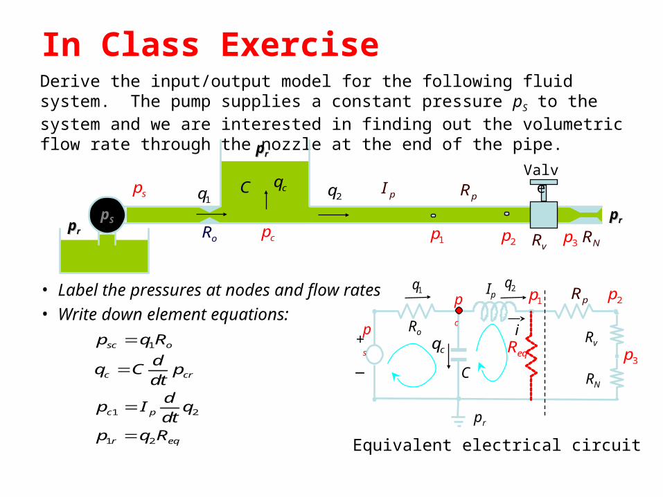
In Class ExerciseDerive the input/output model for the following fluid system. The pump supplies a constant pressure pS to the system and we are interested in finding out the volumetric flow rate through the nozzle at the end of the pipe.

• Label the pressures at nodes and flow rates

• Write down element equations:1

1 2

1 2

sc o

c cr

c p

r eq

p q R

dq C p

dtd

p I qdt

p q R

pSpprr

pprr

pprr

Valve

sp1q

cp

cq2q

2p3p1p

+

_

C

oR

pIpR

vR NR

iRo

C

Rv

pr

ps

1qpc

cq

Ip1p pR 2p

3p

RN

eqR

2q

Equivalent electrical circuit

In Class Exercise• No. of unknowns and equations:

• Interconnection laws:

• Eliminate intermediate variables and obtain I/O model:

Q: Can you draw an equivalent electrical circuit of this hydraulic system ? Note that pressure is analogous to voltage and flow rate is analogues to electric current. (Please refer to the previous slide)

1 1 2 1, , , , , ,sc s cr c rp q q p p q p

Loop 1:

Loop 2:

Node 2:

0sc cr srp p p

1 1 0c r rcp p p

1 2cq q q

we are interested in it

1 1 0cr srR q p p

2 2 0p eq cr

dI q R q p

dt

1 2crdP

q C qdt

2 2cr p eq

dp I q R q

dt

1

1 2 2 2

cr

cr p eq sr

pq

d dR C p q I q R q p

dt dt

2

2 21 1 1 22p eq p eq sr

d q dqR CI R CR I R R q p

dt dt

Motion Control of Hydraulic CylindersHydraulic actuation is attractive for applications when large power is needed while maintaining a reasonable weight. Not counting the weight of the pump and reservoir, hydraulic actuation has the edge in power-to-weight ratio compared with other cost effective actuation sources. Earth moving applications (wheel loaders, excavators, mining equipment, ...) are typical examples where hydraulic actuators are used extensively. A typical motion application involves a hydraulic cylinder connected to certain mechanical linkages (inertia load). The motion of the cylinder is regulated via a valve that is used to regulate the flow rate to the cylinder. It is well known that such system chatters during sudden stop and start. Can you analyze the cause and propose solutions?

M

pS

pprr

RRVVRRVV

Motion Control of Hydraulic Cylinders

Let’s look at a simplified problem:

The input in the system to the right is the input flow rate qIN and the output is the velocity of the mass, V.

A: Cylinder bore area

C: Cylinder chamber capacitance

B: Viscous friction coefficient between piston head and cylinder wall.

• Derive the input/output model and transfer function between qIN and V.

• Draw the block diagram of the system.

• Can this model explain the vibration when we suddenly close the valve?

M

pSr

pprr

RRVV

ppSS

qqININ

AA

ppLLpprr

CCvv

BB

i

C

pr

qIN1qcq

Lp

M

B

vvfc

Motion Control of Hydraulic CylindersElement equations and interconnection equations:

Block diagram representation:

Take Laplace transforms:

Hydraulic system Mechanical systemHydraulic-Mechanical

1

c Lr

IN c

dq C p

dtq q q

1

c Lrf Ap

q Av

cMv f Bv

1

c Lr

IN c

Q s CsP s

Q s Q s Q s

1

c LrF s AP s

Q s AV s

cMsV s F s BV s

Hydraulic System Mechanical SystemH-M Coupling

A LrP s X sQIN(s) 1

Cs

V s

-

A

1

Ms B1

s

V s

cF s

1Q s

Motion Control of Hydraulic CylindersTransfer function between qIN and V:

Analyze the transfer function:Natural Frequency

Damping Ratio

Steady State Gain

How would the velocity response look like if we suddenly open the valve to reach constant input flow rate Q for some time T and suddenly close the valve to stop the flow?

2

2 2

22

2 nn

QVIN

V s AG

Q s MCs BCs A

AMC

B As sM MC

2

n

AAMC MC

2

2 2n

B A B CM BM A MMC

2

1AMCK

A AMC

In reality, large M, small C

very small damping ratio

reasonable value of natural frequency

Oscillation cannot die out quickly

Chattering !!