
Chapter 6 Lagrangian and Hamiltonian Dynamics SO 3mleok/pdf/samplechap.pdf · Chapter 6 Lagrangian...
39
Chapter 6 Lagrangian and Hamiltonian Dynamics on SO(3) This chapter treats the Lagrangian dynamics and Hamiltonian dynamics of a rotating rigid body. A rigid body is a collection of mass particles whose relative positions do not change, that is the body does not deform when acted on by external forces. A rigid body is a useful idealization. The most general form of rigid body motion consists of a combination of rotation and translation. In this chapter, we consider rotational motion only. Combined rotational and translational dynamics of a rigid body are studied in the subsequent chapter. We begin by identifying the configurations of a rotating rigid body in three dimensions as elements of the Lie group SO(3). Equations of motion for the Lagrangian and Hamiltonian dynamics, expressed as Euler–Lagrange (or Euler) equations and Hamilton’s equations, are developed for rigid body rotations in three dimensions. These results are illustrated by several exam- ples of the rotational dynamics of a rigid body. There are many books and research papers that treat rigid body kinematics and dynamics from both theoretical and applied perspectives. It is a common approach in the published literature to describe rigid body kinematics and dynamics in terms of rotation matrices, but not to fully exploit such geometric representations. For example, books such as [5, 10, 26, 30, 32, 70] introduce rotation matrices but make substantial use of local coordinates, such as Eu- ler angles, in analysis and computations. The references [23, 40, 68, 77] are notable for their emphasis on rotation matrices as the primary representation for kinematics and dynamics of rigid body motion on SO(3) in applications to spacecraft and robotics. In the context of multi-body spacecraft control, [84] was one of the first publications formulating multi-body dynamics using the configuration manifold (SO(3)) n . © Springer International Publishing AG 2018 T. Lee et al., Global Formulations of Lagrangian and Hamiltonian Dynamics on Manifolds, Interaction of Mechanics and Mathematics, DOI 10.1007/978-3-319-56953-6 6 273
Transcript of Chapter 6 Lagrangian and Hamiltonian Dynamics SO 3mleok/pdf/samplechap.pdf · Chapter 6 Lagrangian...

Chapter 6
Lagrangian and Hamiltonian Dynamicson SO(3)
This chapter treats the Lagrangian dynamics and Hamiltonian dynamics ofa rotating rigid body. A rigid body is a collection of mass particles whoserelative positions do not change, that is the body does not deform whenacted on by external forces. A rigid body is a useful idealization.
The most general form of rigid body motion consists of a combination ofrotation and translation. In this chapter, we consider rotational motion only.Combined rotational and translational dynamics of a rigid body are studiedin the subsequent chapter.
We begin by identifying the configurations of a rotating rigid body inthree dimensions as elements of the Lie group SO(3). Equations of motionfor the Lagrangian and Hamiltonian dynamics, expressed as Euler–Lagrange(or Euler) equations and Hamilton’s equations, are developed for rigid bodyrotations in three dimensions. These results are illustrated by several exam-ples of the rotational dynamics of a rigid body.
There are many books and research papers that treat rigid body kinematicsand dynamics from both theoretical and applied perspectives. It is a commonapproach in the published literature to describe rigid body kinematics anddynamics in terms of rotation matrices, but not to fully exploit such geometricrepresentations. For example, books such as [5, 10, 26, 30, 32, 70] introducerotation matrices but make substantial use of local coordinates, such as Eu-ler angles, in analysis and computations. The references [23, 40, 68, 77] arenotable for their emphasis on rotation matrices as the primary representationfor kinematics and dynamics of rigid body motion on SO(3) in applicationsto spacecraft and robotics. In the context of multi-body spacecraft control,[84] was one of the first publications formulating multi-body dynamics usingthe configuration manifold (SO(3))n.
© Springer International Publishing AG 2018T. Lee et al., Global Formulations of Lagrangian and HamiltonianDynamics on Manifolds, Interaction of Mechanics and Mathematics,DOI 10.1007/978-3-319-56953-6 6
273

274 6 Lagrangian and Hamiltonian Dynamics on SO(3)
6.1 Configurations as Elements in the Lie Group SO(3)
Two Euclidean frames are introduced; these aid in defining the attitude con-figuration of a rotating rigid body. A reference Euclidean frame is arbitrarilyselected; it is often selected to be an inertial frame but this is not essential.A Euclidean frame fixed to the rigid body is also introduced; this fixed framerotates as the rigid body rotates. The origin of this body-fixed frame can bearbitrarily selected, but it is often convenient to locate it at the center ofmass of the rigid body.
As a manifold embedded in GL(3) or R3×3, recall that
SO(3) ={R ∈ GL(3) : RTR = RRT = I3×3, det(R) = +1
},
has dimension three. The tangent space of SO(3) at R ∈ SO(3) is given by
TRSO(3) ={Rξ ∈ R
3×3 : ξ ∈ so(3)},
and has dimension three. The tangent bundle of SO(3) is given by
TSO(3) ={(R,Rξ) ∈ SO(3)× R
3×3 : ξ ∈ so(3)},
and has dimension six.We can view R ∈ SO(3) as representing the attitude of the rigid body, so
that SO(3) is the configuration manifold for rigid body rotational motion. Anattitude matrix R ∈ SO(3) can be viewed as a linear transformation on R
3 inthe sense that a representation of a vector in the body-fixed frame is trans-formed into a representation of the vector in the reference frame. Thus, thetranspose of an attitude matrix RT ∈ SO(3) denotes a linear transformationfrom a representation of a vector in the reference frame into a representationof the vector in the body-fixed frame. These two important properties aresummarized as:
• If b ∈ R3 is a representation of a vector expressed in the body-fixed frame,
then Rb ∈ R3 denotes the same vector in the reference frame.
• If x ∈ R3 is a representation of a vector expressed in the reference frame,
then RTx ∈ R3 denotes the same vector in the body-fixed frame.
These are important relationships that are used extensively in the subsequentdevelopments.
In addition, R ∈ SO(3) can be viewed as defining a rigid body rotationon R
3 according to the rules of matrix multiplication. In this interpretation,R ∈ SO(3) is viewed as a rotation matrix that defines a linear transformationthat acts on rigid body attitudes. This makes SO(3) a Lie group manifoldusing standard matrix multiplication as the group operation, as discussedin Chapter 1. Since the dimension of SO(3) is three, rigid body rotationalmotion has three degrees of freedom.

6.2 Kinematics on SO(3) 275
6.2 Kinematics on SO(3)
The rotational kinematics of a rotating rigid body are described in terms ofthe time evolution of the attitude and attitude rate of the rigid body givenby (R, R) ∈ TSO(3). As in Chapter 2, the rotational kinematics equationsfor a rotating rigid body are given by
R = Rξ,
where ξ ∈ so(3).We make use of the isomorphism between the Lie algebra so(3) and R
3
given by ξ = S(ω) with ξ ∈ so(3), ω ∈ R3. This perspective is utilized in
the subsequent development. This leads to the expression for the attitude orrotational kinematics given by
R = RS(ω), (6.1)
where ω ∈ R3 is referred to as the angular velocity vector of the rigid body
expressed in the body-fixed Euclidean frame.It is sometimes convenient to partition the rigid body attitude or rotation
R ∈ SO(3) as a 3 × 3 matrix into its rows. We use the notation ri ∈ S2 todenote the i-th column of RT ∈ SO(3) for i = 1, 2, 3. This is equivalent tothe partition
R =
⎡⎣r
T1
rT2rT3
⎤⎦ .
Thus, the rotational kinematics of a rotating rigid body can also be describedby the three vector differential equations
ri = −ξri, i = 1, 2, 3,
or equivalently by
ri = S(ri)ω, i = 1, 2, 3.
We subsequently describe the attitude configuration of a rotating rigidbody by the equivalent descriptions R ∈ SO(3) or ri ∈ S2, i = 1, 2, 3, de-pending on whichever is the most convenient description.

276 6 Lagrangian and Hamiltonian Dynamics on SO(3)
6.3 Lagrangian Dynamics on SO(3)
A Lagrangian function is introduced. Euler–Lagrange equations are derivedusing Hamilton’s principle that the infinitesimal variation of the action inte-gral is zero. The Euler–Lagrange equations are first expressed for an arbitraryLagrangian function; then Euler–Lagrange equations are obtained for the casethat the kinetic energy term in the Lagrangian function is a quadratic func-tion of the angular velocity vector.
6.3.1 Hamilton’s Variational Principle
The Lagrangian function is defined on the tangent bundle of SO(3), that isL : TSO(3) → R
1.We identify the tangent bundle TSO(3) with SO(3)×so(3) or with SO(3)×
R3 using the isomorphism between so(3) and R
3. Thus, we can express theLagrangian as a function L(R, R) = L(R,Rξ) = L(R,RS(ω)) defined on thetangent bundle TSO(3). We make use of the modified Lagrangian functionL(R,ω) = L(R,RS(ω)), where we view L : TSO(3) → R
1 according to thekinematics (6.1).
In studying the dynamics of a rotating rigid body, the Lagrangian functionis the difference of a kinetic energy function and a potential energy function;thus the modified Lagrangian function is
L(R,ω) = T (R,ω)− U(R),
where the kinetic energy function T (R,ω) is viewed as being defined on thetangent bundle TSO(3) and the potential energy function U(R) is defined onSO(3).
The subsequent development describes variations of functions with valuesin the special orthogonal group SO(3); rather than using the abstract Liegroup formalism, we obtain the results explicitly for the rotation group. Inparticular, we introduce variations of a rotational motion t → R(t) ∈ SO(3),denoted by t → Rε(t) ∈ SO(3), by using the exponential map and the iso-morphism between so(3) and R
3.The variation of R : [t0, tf ] → SO(3) is a differentiable curve Rε : (−c, c)×
[t0, tf ] → SO(3) for c > 0 such that R0(t) = R(t), and Rε(t0) = R(t0),Rε(tf ) = R(tf ) for any ε ∈ (−c, c).
The variation of a rotational motion can be described using the exponentialmap as
Rε(t) = R(t)eεS(η(t)),

6.3 Lagrangian Dynamics on SO(3) 277
where ε ∈ (−c, c) and η : [t0, tf ] → R3 is a differentiable curve that vanishes
at t0 and tf . Consequently, S(η(t)) ∈ so(3) defines a differentiable curve withvalues in the Lie algebra of skew symmetric matrices that vanishes at t0 andtf , and eεS(η(t)) ∈ SO(3) defines a differentiable curve that takes values inthe Lie group of rotation matrices and is the identity matrix at t0 and tf .Thus, the time derivative of the variation of the rotational motion of a rigidbody is
Rε(t) = R(t)eεS(η(t)) + εR(t)eεS(η(t))S(η(t)).
Suppressing the time dependence in the subsequent notation, the varied curvesatisfies
ξε = (Rε)T Rε
= e−εS(η)ξeεS(η) + εS(η)
= ξ + ε (S(η) + ξS(η)− S(η)ξ) +O(ε2).
Define the variation of the angular velocity by ξε = S(ωε) and use the factthat ξ = S(ω) to obtain
S(ωε) = S(ω) + ε(S(η) + S(ω)S(η)− S(η)S(ω)) +O(ε2).
We use a skew symmetric matrix identity to obtain
S(ωε) = S(ω) + ε(S(η) + S(ω × η)) +O(ε2),
or equivalently
S(ωε) = S(ω + ε(η + ω × η)) +O(ε2).
Thus, the variation of the angular velocity satisfies
ωε = ω + ε (η + ω × η) +O(ε2).
From these expressions, we determine the infinitesimal variations
δR =d
dεRε
∣∣∣∣ε=0
= RS(η), (6.2)
δω =d
dεωε
∣∣∣∣ε=0
= η + ω × η = η + S(ω)η. (6.3)
This framework allows us to introduce the action integral and Hamilton’sprinciple to obtain Euler–Lagrange equations that describe the rotationaldynamics of a rigid body.
The action integral is the integral of the Lagrangian function, or equiv-alently the modified Lagrangian function, along a rotational motion of the

278 6 Lagrangian and Hamiltonian Dynamics on SO(3)
rigid body over a fixed time period. The variations are taken over all differ-entiable curves with values in SO(3) for which the initial and final values arefixed.
The action integral along a rotational motion of a rotating rigid body is
G =
∫ tf
t0
L(R,ω) dt.
The action integral along a variation of a rotational motion of the rigid body is
Gε =
∫ tf
t0
L(Rε, ωε) dt.
The varied value of the action integral along a variation of a rotational motionof the rigid body can be expressed as a power series in ε as
Gε = G+ εδG+O(ε2),
where the infinitesimal variation of the action integral is
δG =d
dεGε
∣∣∣∣ε=0
.
Hamilton’s principle states that the infinitesimal variation of the action in-tegral along any rotational motion of the rigid body is zero:
δG =d
dεGε
∣∣∣∣ε=0
= 0, (6.4)
for all possible infinitesimal variations η : [t0, tf ] → R3 satisfying η(t0) =
η(tf ) = 0.
6.3.2 Euler–Lagrange Equations: General Form
We first compute the infinitesimal variation of the action integral as
d
dεGε
∣∣∣∣ε=0
=
∫ tf
t0
{∂L(R,ω)
∂ω· δω +
∂L(R,ω)
∂R· δR
}dt.
Examining the first term, we obtain

6.3 Lagrangian Dynamics on SO(3) 279
∫ tf
t0
∂L(R,ω)
∂ω· δω dt =
∫ tf
t0
∂L(R,ω)
∂ω· (η + ω × η) dt
= −∫ tf
t0
{d
dt
(∂L(R,ω)
∂ω
)+ S(ω)
∂L(R,ω)
∂ω
}· η dt,
where the first term is integrated by parts, using the fact that η(t0) = η(tf ) =0, and the second term is rewritten using a cross product identity.
The second term above is now rewritten. We use the notation ri ∈ S2 andδri ∈ TriS
2 to denote the i-th column of RT ∈ SO(3) and δRT ∈ TRSO(3),respectively. This is equivalent to partitioning R and δR into row vectors as
R =
⎡⎣r
T1
rT2rT3
⎤⎦ , δR =
⎡⎣δr
T1
δrT2δrT3
⎤⎦ .
We use the fact that δri = S(ri)η to obtain
∫ tf
t0
∂L(R,ω)
∂R· δR dt =
∫ tf
t0
3∑i=1
∂L(R,ω)
∂ri· δri dt
=
∫ tf
t0
3∑i=1
∂L(R,ω)
∂ri· S(ri)η dt
= −∫ tf
t0
3∑i=1
(S(ri)
∂L(R,ω)
∂ri
)· η dt. (6.5)
Substituting, the expression for the infinitesimal variation of the action inte-gral is obtained:
d
dεGε
∣∣∣∣ε=0
= −∫ tf
t0
{d
dt
(∂L(R,ω)
∂ω
)+ S(ω)
∂L(R,ω)
∂ω+
3∑i=1
S(ri)∂L(R,ω)
∂ri
}· η dt.
From Hamilton’s principle, the above expression for the infinitesimal vari-ation of the action integral should be zero for all differentiable variationsη : [t0, tf ] → R
3 with fixed endpoints. The fundamental lemma of the calcu-lus of variations leads to the Euler–Lagrange equations.
Proposition 6.1 The Euler–Lagrange equations for a modified Lagrangianfunction L : TSO(3) → R
1 are
d
dt
(∂L(R,ω)
∂ω
)+ ω × ∂L(R,ω)
∂ω+
3∑i=1
ri × ∂L(R,ω)
∂ri= 0. (6.6)

280 6 Lagrangian and Hamiltonian Dynamics on SO(3)
This form of the Euler–Lagrange equations, together with the rotational kine-matics equations (6.1), describe the Lagrangian flow of a rotating rigid bodyon the tangent bundle TSO(3) in terms of (R,ω) ∈ TSO(3).
6.3.3 Euler–Lagrange Equations: Quadratic Kinetic Energy
We now determine a more explicit expression for the kinetic energy of arotating rigid body. This expression is used to obtain a standard form of theEuler–Lagrange equations. For simplicity, the reference frame is assumed tobe an inertial frame, and the origin of the body-fixed frame is assumed to belocated at the center of mass of the rigid body.
Let ρ ∈ B ⊂ R3 be a vector from the origin of the body-fixed frame to
a mass element of the rigid body expressed in the body-fixed frame. HereB denotes the set of material points that constitute the rigid body in thebody-fixed frame. Thus, Rρ is the velocity vector of this mass element in theinertial frame. The kinetic energy of the rotating rigid body can be expressedas the body integral
T (R,ω) =1
2
∫B‖Rρ‖2 dm(ρ)
=1
2
∫B‖RS(ρ)ω‖2 dm(ρ)
=1
2ωT
(∫BS(ρ)TS(ρ) dm(ρ)
)ω,
where dm(ρ) denotes the mass of the incremental element located at ρ ∈ B.Thus, we can express the kinetic energy as a quadratic function of the angularvelocity vector
T (R,ω) =1
2ωTJω,
where
J =
∫BS(ρ)TS(ρ) dm(ρ),
is the 3× 3 standard inertia matrix of the rigid body that characterizes therotational inertia of the rigid body in the body-fixed frame.
The inertia matrix can be shown to be a symmetric and positive-definitematrix. It has three positive eigenvalues and three eigenvectors that form anorthonormal basis for R3. This special basis defines the principal axes of therigid body and it is sometimes convenient to select the body-fixed frame to

6.4 Hamiltonian Dynamics on SO(3) 281
be aligned with the principal axes of the body. In this case, the inertia matrixis diagonal.
Consequently, the modified Lagrangian function has the special form
L(R,ω) =1
2ωTJω − U(R). (6.7)
This gives the standard form of the equations for a rotating rigid body, oftenreferred to as the Euler equations for rigid body rotational dynamics, as
Jω + S(ω)Jω −3∑
i=1
S(ri)∂U(R)
∂ri= 0. (6.8)
These Euler equations (6.8), together with the rotational kinematics (6.1),describe the Lagrangian flow of a rotating rigid body in terms of the evolutionof (R,ω) ∈ TSO(3) on the tangent bundle TSO(3).
If the potential energy terms in (6.8) are globally defined on R3×3, then
the domain of definition of the rotational kinematics (6.1) and the Eulerequations (6.8) on TSO(3) can be extended to TR3×3. This extension is nat-ural and useful in that it defines a Lagrangian vector field on the tangentbundle TR3×3 Alternatively, the manifold TSO(3) is an invariant manifoldof this Lagrangian vector field on TR3×3 and its restriction to this invariantmanifold describes the Lagrangian flow of (6.1) and (6.8) on TSO(3).
6.4 Hamiltonian Dynamics on SO(3)
We introduce the Legendre transformation to obtain the angular momen-tum and the Hamiltonian function. We make use of Hamilton’s phase spacevariational principle to derive Hamilton’s equations for a rotating rigid body.
6.4.1 Hamilton’s Phase Space Variational Principle
As in the prior section, we begin with a modified Lagrangian function L :TSO(3) → R
1, which is a real-valued function defined on the tangent bundleof the configuration manifold SO(3); we assume that the modified Lagrangianfunction
L(R,ω) = T (R,ω)− U(R),
is given by the difference between a kinetic energy function T (R,ω) defined onthe tangent bundle and a configuration dependent potential energy functionU(R).

282 6 Lagrangian and Hamiltonian Dynamics on SO(3)
The angular momentum of the rotating rigid body in the body-fixed frameis defined by the Legendre transformation
Π =∂L(R,ω)
∂ω, (6.9)
where we assume the Lagrangian has the property that the map ω ∈ so(3) →Π ∈ so(3)∗ is invertible. The angular momentum is viewed as being conjugateto the angular velocity vector.
The modified Hamiltonian function H : T∗SO(3) → R1 is defined on the
cotangent bundle of SO(3) by
H(R,Π) = Π · ω − L(R,ω),
using the Legendre transformation.Consider the modified action integral of the form,
G =
∫ tf
t0
{Π · ω − H(R,Π)
}dt.
The infinitesimal variation of the action integral is given by
δG =
∫ tf
t0
{Π · δω − ∂H(R,Π)
∂R· δR+ δΠ ·
(ω − ∂H(R,Π)
∂Π
)}dt.
Recall from (6.2) and (6.3) that the infinitesimal variations can be written as
δR = RS(η),
δω = η + S(ω)η,
for differentiable curves η : [t0, tf ] → R3. Following the arguments used to
obtain (6.5),
∫ tf
t0
∂H(R,Π)
∂R· δR dt = −
∫ tf
t0
3∑i=1
(S(ri)
∂H(R,Π)
∂ri
)· η dt.
6.4.2 Hamilton’s Equations: General Form
We now derive Hamilton’s equations. Substitute the preceding expressionsinto the expression for the infinitesimal variation of the modified action inte-gral and integrate by parts to obtain
δG =
∫ tf
t0
Π · (η + S(ω)η) +
3∑i=1
(S(ri)
∂H(R,Π)
∂ri
)· η

6.4 Hamiltonian Dynamics on SO(3) 283
+ δΠ ·(ω − ∂H(R,Π)
∂Π
)dt
=
∫ tf
t0
{−Π − S(ω)Π +
3∑i=1
(S(ri)
∂H(R,Π)
∂ri
)}· η
+ δΠ ·(ω − ∂H(R,Π)
∂Π
)dt.
Invoke Hamilton’s phase space variational principle that δG = 0 for allpossible functions η : [t0, tf ] → R
3 and δΠ : [t0, tf ] → R3 that satisfy
η(t0) = η(tf ) = 0. This implies that the expression in each of the bracesof the above equation should be zero. We thus obtain Hamilton’s equations,expressed in terms of (R,Π).
Proposition 6.2 Hamilton’s equations for a modified Hamiltonian functionH : T∗SO(3) → R
1 are
ri = ri × ∂H(R,Π)
∂Π, i = 1, 2, 3, (6.10)
Π = Π × ∂H(R,Π)
∂Π+
3∑i=1
ri × ∂H(R,Π)
∂ri. (6.11)
Thus, equations (6.10) and (6.11) define Hamilton’s equations of motion forthe dynamics of the Hamiltonian flow in terms of the evolution of (R,Π) ∈T∗SO(3) on the cotangent bundle TSO(3).
The following property follows directly from the above formulation ofHamilton’s equations on SO(3):
dH(R,Π)
dt=
3∑i=1
∂H(R,Π)
∂ri· ri + ∂H(R,Π)
∂Π· Π
=∂H(R,Π)
∂Π· S(Π)
∂H(R,Π)
∂Π= 0.
The modified Hamiltonian function is constant along each solution of Hamil-ton’s equation. This property does not hold if the modified Hamiltonian func-tion has a nontrivial explicit dependence on time.

284 6 Lagrangian and Hamiltonian Dynamics on SO(3)
6.4.3 Hamilton’s Equations: Quadratic Kinetic Energy
Suppose the kinetic energy is a quadratic in the angular velocity vector
L(R,ω) =1
2ωTJω − U(R).
The Legendre transformation gives
Π = Jω,
and the modified Hamiltonian function can be expressed as
H(R,Π) =1
2ΠTJ−1Π + U(R). (6.12)
Hamilton’s equations for a rotating rigid body are described on the cotangentbundle T∗SO(3) as:
ri = ri × J−1Π, i = 1, 2, 3, (6.13)
Π = Π × J−1Π +
3∑i=1
ri × ∂U(R)
∂ri. (6.14)
Equations (6.13) and (6.14) define Hamilton’s equations of motion for rigidbody dynamics and they describe the Hamiltonian flow in terms of the evo-lution of (R,Π) ∈ T∗SO(3) on the cotangent bundle T∗SO(3).
If the potential energy terms in (6.14) are globally defined on R3×3, then
the domain of definition of (6.13) and (6.14) on T∗SO(3) can be extendedto T∗
R3×3. This extension is natural and useful in that it defines a Hamilto-
nian vector field on the cotangent bundle T∗R
3×3 Alternatively, the manifoldT∗SO(3) is an invariant manifold of this Hamiltonian vector field on T∗
R3×3
and its restriction to this invariant manifold describes the Hamiltonian flowof (6.13) and (6.14) on T∗SO(3).
6.5 Linear Approximations of Dynamics on SO(3)
Geometric forms of the Euler–Lagrange equations and Hamilton’s equationson the configuration manifold SO(3) have been presented. This yields equa-tions of motion that provide insight into the geometry of the global dynamicson SO(3).
A linear vector field can be determined that approximates the Lagrangianvector field on TSO(3), at least locally in an open subset of TSO(3). Such lin-ear approximations allow a straightforward analysis of local dynamics prop-erties.

6.6 Dynamics on SO(3) 285
A common approach in the literature on the dynamics of rotating rigidbodies involves introducing local coordinates in the form of three angle coor-dinates; the most common local coordinates are Euler angles, but exponentiallocal coordinates have some advantages as described in Appendix B. Thesedescriptions often involve complicated trigonometric or transcendental ex-pressions and introduce complexity in the analysis and computations.
Although our main emphasis is on global methods, we make use of localcoordinates as a way of describing a linear vector field that approximatesa vector field on TSO(3), at least in the neighborhood of an equilibriumsolution. This approach is used subsequently in this chapter to study thelocal flow properties near an equilibrium. As further background, linearizedequations are developed in local coordinates for SO(3) in Appendix B.
6.6 Dynamics on SO(3)
We study several physical examples of a rotating rigid body in three dimen-sions. In each, the configuration manifold is SO(3); consequently each of thedynamics has three degrees of freedom. Lagrangian and Hamiltonian formu-lations of the equations of motion are presented; a few simple flow propertiesare identified.
6.6.1 Dynamics of a Freely Rotating Rigid Body
We consider a freely rotating rigid body, also referred to as the free rigidbody, in the sense that no moments act on the body. In this case, the priordevelopment holds with zero potential energy U(R) = 0. This is the simplestcase of a rotating rigid body in three dimensions.
An inertial Euclidean frame is selected arbitrarily. The origin of the body-fixed Euclidean frame is assumed to be located at the center of mass of therigid body which is assumed to be fixed in the inertial frame. A schematic ofa freely rotating rigid body is shown in Figure 6.1.
6.6.1.1 Euler–Lagrange Equations
The attitude kinematics equation for the free rigid body is described by
R = RS(ω). (6.15)
The modified Lagrangian function L : TSO(3) → R1 is
L(R,ω) =1
2ωTJω.

286 6 Lagrangian and Hamiltonian Dynamics on SO(3)
R ∈ SO(3)
Fig. 6.1 Freely rotating rigid body
Following the results in (6.8) with zero potential energy, the Euler–Lagrangeequations of motion for the free rigid body, referred to as the Euler equations,are given by
Jω + ω × Jω = 0, (6.16)
where J =∫B S(ρ)TS(ρ)dm(ρ) is the standard 3 × 3 inertia matrix of the
rigid body in the body-fixed frame. These equations of motion (6.15) and(6.16) define the Lagrangian flow for the free rigid body dynamics describedby the evolution of (R,ω) ∈ TSO(3) on the tangent bundle of SO(3).
6.6.1.2 Hamilton’s Equations
Using the Legendre transformation, let
Π =∂L(R,ω)
∂ω= Jω
be the angular momentum of the free rigid body expressed in the body-fixedframe. The modified Hamiltonian is
H(R,Π) =1
2ΠTJ−1Π.
The rotational kinematics equation can be written as
R = RS(J−1Π). (6.17)
Using (6.16), Hamilton’s equations are given by
Π = Π × J−1Π, (6.18)

6.6 Dynamics on SO(3) 287
Thus, Hamilton’s equations of motion (6.17) and (6.18) describe the Hamil-tonian dynamics of the free rigid body as (R,Π) ∈ T∗SO(3) as they evolveon the cotangent bundle of SO(3).
6.6.1.3 Conservation Properties
There are two conserved quantities, or integrals of motion, for the rotationaldynamics of a free rigid body. First, the Hamiltonian, which is the rotationalkinetic energy and coincides with the total energy E in this case, is conserved;that is
H =1
2ωTJω
is constant along each solution of the dynamical flow of the free rigid body.In addition, there is a rotational symmetry: the Lagrangian is invariant
with respect to the tangent lift of arbitrary rigid body rotations. This sym-metry leads to conservation of the angular momentum in the inertial frame;that is
RΠ = RJω
is constant along each solution of the dynamical flow of the free rigid body.Consequently the magnitude of the angular momentum in the body-fixedframe is also conserved, that is
‖Jω‖2
is constant along each solution of the dynamical flow of the free rigid body.These results are well known for the free rigid body and they guarantee thatthe free rigid body is integrable [10].
There are additional conservation properties if the distribution of mass inthe rigid body has a symmetry. There are many published results for suchcases.
6.6.1.4 Equilibrium Properties
The equilibria or constant solutions are easily identified. The free rigid bodyis in equilibrium at any attitude in SO(3) if the angular velocity vector iszero.
To illustrate the linearization of the dynamics of a rotating rigid body, con-sider the equilibrium solution (I3×3, 0) ∈ TSO(3). According to Appendix B,θ = (θ1, θ2, θ3) ∈ R
3 are exponential local coordinates for SO(3) in a neigh-borhood of I3×3 ∈ SO(3). Following the results in Appendix B, the linearizeddifferential equations defined on the six-dimensional tangent space of TSO(3)

288 6 Lagrangian and Hamiltonian Dynamics on SO(3)
at (I3×3, 0) ∈ TSO(3) are given by
Jξ = 0.
These linearized differential equations approximate the rotational dynamicsof the rigid body in a neighborhood of (I3×3, 0) ∈ TSO(3). These simplelinear dynamics are accurate to first-order in the perturbations expressed inlocal coordinates. Higher-order coupling effects are important for large per-turbations of the angular velocity vector of the rigid body from equilibrium.
Solutions for which the angular velocity vector are constant can also beidentified; these are referred to as relative equilibrium solutions and theynecessarily satisfy
ω × Jω = 0.
Thus, the relative equilibrium solutions occur when the angular velocity vec-tor is collinear with an eigenvector of the inertia matrix J . A comprehensivetreatment of relative equilibria of the free rigid body is given in [36].
6.6.2 Dynamics of a Three-Dimensional Pendulum
A three-dimensional pendulum is a rigid body supported by a fixed, fric-tionless pivot, acted on by uniform, constant gravity. The terminology three-dimensional pendulum refers to the fact that the pendulum is a rigid body,with three rotational degrees of freedom, that rotates under uniform, constantgravity. The formulation of a three-dimensional pendulum seems first to havebeen introduced in [87] and its dynamics developed further in [18, 20, 21, 58].The development that follows is based on these sources.
An inertial Euclidean frame is selected so that the first two axes lie ina horizontal plane and the third axis is vertical. The origin of the inertialEuclidean frame is selected to be the location of the pendulum pivot. Thebody-fixed frame is selected so that its origin is located at the center of massof the rigid body. Let m be the mass of the three-dimensional pendulum andlet ρ0 ∈ R
3 be the nonzero vector from the center of mass of the body to thepivot, expressed in the body-fixed frame. Let J be the constant 3× 3 inertiamatrix of the rigid body described subsequently. As before, g denotes the con-stant acceleration of gravity. A schematic of a three-dimensional pendulumis shown in Figure 6.2.
The attitude of the rigid body is R ∈ SO(3) and ω ∈ R3 is the angular
velocity vector of the rigid body. The attitude kinematics equation for thethree-dimensional pendulum is
R = RS(ω). (6.19)

6.6 Dynamics on SO(3) 289
R ∈ SO(3)
Fig. 6.2 Three-dimensional pendulum
6.6.2.1 Euler–Lagrange Equations
Let ρ ∈ R3 be a vector from the origin of the body-fixed frame to a mass
element of the rigid body expressed in the body-fixed frame. Thus, R(−ρ0+ρ)is the velocity vector of this mass element in the inertial frame. The kineticenergy of the rotating rigid body can be expressed as the body integral
T (R,ω) =1
2
∫B‖R(−ρ0 + ρ)‖2 dm(ρ)
=1
2
∫B‖RS(−ρ0 + ρ)ω‖2 dm(ρ)
=1
2ωTJω,
where the moment of inertia matrix is
J =
∫BS(ρ)TS(ρ)dm(ρ) +mST (ρ0)S(ρ0).
The gravitational potential energy of the three-dimensional pendulumarises from the gravitational field acting on each material particle in thependulum body. This can be expressed as
U(R) = −∫BgeT3 Rρdm(ρ) = −mgeT3 Rρ0.
The modified Lagrangian function of the three-dimensional pendulum canbe expressed as:
L(R,ω) =1
2ωTJω +mgeT3 Rρ0.
The Euler–Lagrange equations for the three-dimensional pendulum are givenby
Jω + ω × Jω −mgρ0 ×RT e3 = 0. (6.20)
290 6 Lagrangian and Hamiltonian Dynamics on SO(3)
These equations (6.19) and (6.20) define the rotational kinematics andthe Lagrangian dynamics of the three-dimensional pendulum described by(R,ω) ∈ TSO(3).
6.6.2.2 Hamilton’s Equations
Hamilton’s equations of motion are easily obtained. According to the Legen-dre transformation,
Π =∂L(R,ω)
∂ω= Jω
is the angular momentum of the three-dimensional pendulum expressed inthe body-fixed frame. Thus, the modified Hamiltonian is
H(R,Π) =1
2ΠTJ−1Π −mgS(ρ0)R
T e3.
Hamilton’s equations of motion are given by the rotational kinematics
R = RS(J−1Π). (6.21)
and
Π = Π × J−1Π +mgρ0 ×RT e3, (6.22)
Thus, the Hamiltonian dynamics of the three-dimensional pendulum, de-scribed by equations (6.21) and (6.22), characterize the evolution of (R,Π)on the cotangent bundle T∗SO(3).
6.6.2.3 Conservation Properties
There are two conserved quantities, or integrals of motion, for the three-dimensional pendulum. First, the Hamiltonian, which coincides with the totalenergy E in this case, is conserved, that is
H =1
2ωTJω −mgρT0 R
T e3,
and it is constant along each solution of the dynamical flow of the three-dimensional pendulum.
In addition, the modified Lagrangian is invariant with respect to the liftedaction of rotations about the vertical or gravity direction. By Noether’s the-orem, this symmetry leads to conservation of the component of angular mo-mentum about the vertical or gravity direction; that is

6.6 Dynamics on SO(3) 291
h = ωTJRT e3,
and it is constant along each solution of the dynamical flow of the three-dimensional pendulum.
6.6.2.4 Equilibrium Properties
The equilibrium or constant solutions of the three-dimensional pendulum areeasily obtained. The conditions for an equilibrium solution are:
ω × Jω −mgρ0 ×RT e3 = 0,
RS(ω) = 0.
Since R ∈ SO(3) is non-singular, it follows that the angular velocity vectorω = 0. Thus, an equilibrium attitude satisfies
ρ0 ×RT e3 = 0,
which implies that
RT e3 =ρ0‖ρ0‖ ,
or
RT e3 = − ρ0‖ρ0‖ .
An attitude R is an equilibrium attitude if and only if the vertical directionor equivalently the gravity direction RT e3, resolved in the body-fixed frame,is collinear with the body-fixed vector ρ0 from the center of mass of therigid body to the pivot. If RT e3 is in the opposite direction to the vectorρ0, then (R, 0) ∈ TSO(3) is an inverted equilibrium of the three-dimensionalpendulum; if RT e3 is in the same direction to the vector ρ0, then (R, 0) is ahanging equilibrium of the three-dimensional pendulum.
Without loss of generality, it is convenient to assume that the constantcenter of mass vector, in the body-fixed frame, satisfies
ρ0‖ρ0‖ = −e3.
Consequently, if R ∈ SO(3) defines an equilibrium attitude for the three-dimensional pendulum, then an arbitrary rotation of the three-dimensionalpendulum about the vertical is also an equilibrium attitude. In summary,there are two disjoint equilibrium manifolds for the three-dimensional pen-dulum.
292 6 Lagrangian and Hamiltonian Dynamics on SO(3)
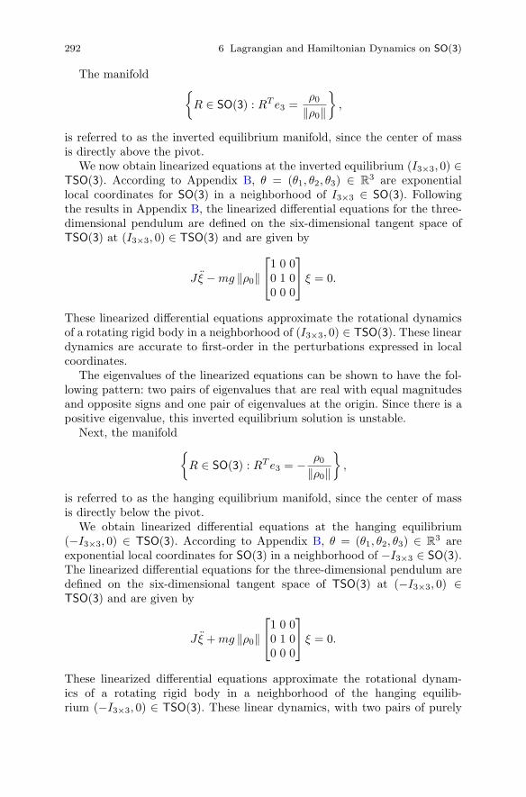
The manifold {R ∈ SO(3) : RT e3 =
ρ0‖ρ0‖
},
is referred to as the inverted equilibrium manifold, since the center of massis directly above the pivot.
We now obtain linearized equations at the inverted equilibrium (I3×3, 0) ∈TSO(3). According to Appendix B, θ = (θ1, θ2, θ3) ∈ R
3 are exponentiallocal coordinates for SO(3) in a neighborhood of I3×3 ∈ SO(3). Followingthe results in Appendix B, the linearized differential equations for the three-dimensional pendulum are defined on the six-dimensional tangent space ofTSO(3) at (I3×3, 0) ∈ TSO(3) and are given by
Jξ −mg ‖ρ0‖⎡⎣1 0 00 1 00 0 0
⎤⎦ ξ = 0.
These linearized differential equations approximate the rotational dynamicsof a rotating rigid body in a neighborhood of (I3×3, 0) ∈ TSO(3). These lineardynamics are accurate to first-order in the perturbations expressed in localcoordinates.
The eigenvalues of the linearized equations can be shown to have the fol-lowing pattern: two pairs of eigenvalues that are real with equal magnitudesand opposite signs and one pair of eigenvalues at the origin. Since there is apositive eigenvalue, this inverted equilibrium solution is unstable.
Next, the manifold
{R ∈ SO(3) : RT e3 = − ρ0
‖ρ0‖},
is referred to as the hanging equilibrium manifold, since the center of massis directly below the pivot.
We obtain linearized differential equations at the hanging equilibrium(−I3×3, 0) ∈ TSO(3). According to Appendix B, θ = (θ1, θ2, θ3) ∈ R
3 areexponential local coordinates for SO(3) in a neighborhood of −I3×3 ∈ SO(3).The linearized differential equations for the three-dimensional pendulum aredefined on the six-dimensional tangent space of TSO(3) at (−I3×3, 0) ∈TSO(3) and are given by
Jξ +mg ‖ρ0‖⎡⎣1 0 00 1 00 0 0
⎤⎦ ξ = 0.
These linearized differential equations approximate the rotational dynam-ics of a rotating rigid body in a neighborhood of the hanging equilib-rium (−I3×3, 0) ∈ TSO(3). These linear dynamics, with two pairs of purely

6.6 Dynamics on SO(3) 293
imaginary eigenvalues and one pair of zero eigenvalues, are accurate to first-order in the perturbations expressed in local coordinates.
Solutions for which the angular velocity vector are constant can also beidentified; these are relative equilibrium solutions and they necessarily satisfy
ω × Jω −mgρ0 ×RT e3 = 0.
Thus, the relative equilibrium solutions occur when the angular velocity vec-tor is collinear with an eigenvector of the inertia matrix J , and the directionof this angular velocity vector, in the inertial frame, is collinear with thegravity direction.
6.6.3 Dynamics of a Rotating Rigid Body in Orbit
Consider the rotational motion of a rigid body in a circular orbit about alarge central body. A Newtonian gravity model is used, which gives rise to adifferential gravity force on each mass element of the rigid body; this grav-ity gradient moment is included in our subsequent analysis. The subsequentdevelopment follows the presentations in [50, 51].
Three Euclidean frames are introduced: an inertial frame whose origin isat the center of the central body, a body-fixed frame whose origin is locatedat the center of mass of the orbiting rigid body, and a so-called local vertical,local horizontal (LVLH) frame, whose first axis is tangent to the circularorbit, the second axis is perpendicular to the plane of the orbit, and thethird axis is along the orbit radius vector. The origin of the LVLH frame islocated at the center of mass of the rigid body and remains on the circularorbit, so that the LVLH frame necessarily rotates at the orbital rate. TheLVLH frame is not an inertial frame, but it does have physical significance;it is used to describe the gravity gradient moment. A schematic of a rotatingrigid body in a circular orbit is shown in Figure 6.3.
Fig. 6.3 Rotating rigid body in a circular orbit

294 6 Lagrangian and Hamiltonian Dynamics on SO(3)
We define three sets of rotation matrices in SO(3): Rbi ∈ SO(3) denotes arotation matrix from the body-fixed frame to the inertial frame, Rli ∈ SO(3)denotes a rotation matrix from the LVLH frame to the inertial frame, andRbl ∈ SO(3) denotes a rotation matrix from the body-fixed frame to theLVLH frame. Thus, the three rotation matrices satisfy Rbl = (Rli)TRbi. Weshow that the dynamics of a rotating rigid body in a circular orbit can beexpressed in terms of the rotation matrix Rbi ∈ SO(3), so that SO(3) is theconfiguration manifold.
Let ω ∈ R3 be the angular velocity of the rigid body expressed in the
body-fixed frame. The 3×3 constant matrix J is the standard inertia matrixof the rigid body in the body-fixed frame. The scalar orbital angular velocity
is ω0 =√
GMr30
, where M denotes the mass of the central body, G is the
universal gravitational constant, and r0 is the constant radius of the circularorbit. The inertial frame is selected so that the orbital plane is orthogonalto the second inertial axis; hence the orbital angular velocity vector is ω0e2in the inertial frame. The LVLH frame is selected so that the orbit radiusvector of the body is r0e3 in the LVLH frame.
6.6.3.1 Euler–Lagrange Equations
Based on the prior developments in this chapter, the on-orbit rigid bodyrotational kinematics equations are given as follows. The attitude of the body-fixed frame with respect to the inertial frame is described by the rotationalkinematics
Rbi = RbiS(ω),
the attitude of the LVLH frame with respect to the inertial frame is describedby the rotational kinematics
Rli = RliS(ω0e2),
and the attitude of the body-fixed frame with respect to the LVLH frame isdescribed by the rotational kinematics
Rbl =RblS(ω − ω0RblT e2).
The modified Lagrangian L : TSO(3) → R1 is given by
L(Rbi, ω) =1
2ωTJω − U(Rbi),
where U(Rbi) is the gravitational potential energy of the rigid body in orbit.Thus, the Euler–Lagrange equations of motion are given by

6.6 Dynamics on SO(3) 295
Jω + ω × Jω = Mg,
where
Mg =3∑
i=1
ri × ∂U(Rbi)
∂ri,
is the gravity gradient moment on the rigid body due to the gravity poten-tial U(Rbi). In the gravity gradient moment expression, r1, r2, r3 denote thecolumn partitions of (Rbi)T ∈ SO(3).
Since the orbital angular velocity ω0 is constant, the rotational kinematicsequation for Rli ∈ SO(3) can be explicitly solved to obtain
Rli(t) = Rli(t0)eS(ω0e2)(t−t0).
This describes the rotation of the LVLH frame with respect to the inertialframe.
The gravity potential for the full orbiting rigid body is obtained by inte-grating the gravity potential for each element in the body over the body; thisleads to
U(Rbi) = −∫B
GM
‖x+Rbiρ‖ dm(ρ),
where x ∈ R3 is the position of the center of mass of the orbiting rigid body
in the inertial frame, and ρ ∈ R3 is a vector from the center of mass of the
rigid body to the body element with mass dm(ρ) in the body-fixed frame.We now derive a closed form approximation for the gravitational moment
Mg using the fact that the rigid body is in a circular orbit so that the normof x is constant. The size of the rigid body is assumed to be much smallerthan the orbital radius.
Since the rigid body position vector in the LVLH frame is r0e3, the positionvector of the rigid body in the inertial frame is given by x = r0R
lie3. Usingthis expression, the matrix of derivatives of the gravitational potential energyis
∂U(Rbi)
∂Rbi=
∫B
GM r0Rli e3ρ
T
‖ r0e3 +Rblρ ‖3dm(ρ)
=GM
r0
∫B
(Rlie3ρ
T) ‖ρ‖
r0[1 + 2
(eT3 R
blρ) ‖ρ‖
r0+ ‖ρ‖2
r20
] 32
dm(ρ),
where ρ = ρ‖ρ‖ ∈ R
3 is the unit vector along the direction of ρ. Since the size
of the rigid body is significantly smaller than the orbital radius, it follows
that ‖ρ‖r0
1. Using a Taylor series expansion, we obtain the second-orderapproximation:

296 6 Lagrangian and Hamiltonian Dynamics on SO(3)
∂U(Rbi)
∂Rbi=
GM
r0
∫BRlie3ρ
T
{‖ρ‖r0
− 3eT3 Rblρ
‖ρ‖2r20
}dm(ρ).
Since the body-fixed frame is located at the center of mass of the rigid body,∫B ρ dm(ρ) = 0. Therefore, the first term in the above equation vanishes.
Since eT3 Rblρ is a scalar, it can be shown that the above partial derivative
matrix can be written as
∂U(Rbi)
∂Rbi= −3ω2
0Rlie3e
T3 R
bl
(1
2tr[J ] I3×3 − J
).
This can be used to obtain an expression for the gravity gradient moment onthe full rigid body:
Mg =
3∑i=1
ri × ∂U(Rbi)
∂ri= 3ω2
0RblT e3 × JRblT e3.
In summary, the Euler equations can be written as
Jω + ω × Jω = 3ω20R
blT e3 × JRblT e3, (6.23)
and the attitude kinematics equation with respect to the LVLH frame is
Rbl = RblS(ω − ω0RblT e2). (6.24)
These rotational equations of motion (6.23) and (6.24) define the Lagrangianflow of an on-orbit rigid body as the dynamics described by (Rbl, ω) ∈ TSO(3)evolve on the tangent bundle of SO(3). Rotational dynamics that describe theattitude of the rigid body in the inertial frame or in the body-fixed framecan be obtained from the above development.
6.6.3.2 Hamilton’s Equations
Hamilton’s equations are easily obtained by defining the angular momentum
Π =∂L(R,ω)
∂ω= Jω.
Thus, the modified Hamiltonian function is
H(Rbi, Π) =1
2ΠTJ−1Π + U(Rbi).
Hamilton’s equations of motion for the on-orbit rigid body can be written asthe attitude kinematics equation with respect to the LVLH frame, namely

6.6 Dynamics on SO(3) 297
Rbl = RblS(J−1Π − ω0RblT e2), (6.25)
and the Euler equations
Π = Π × J−1Π + 3ω20R
blT e3 × JRblT e3. (6.26)
These equations (6.25) and (6.26) define the Hamiltonian flow of the rota-tional dynamics of an on-orbit rigid body as described by (Rbl, Π) ∈ T∗SO(3)on the cotangent bundle of SO(3). Rotational dynamics that describe the at-titude of the rigid body in the inertial frame or in the body-fixed frame canbe obtained from the above development.
6.6.3.3 Conservation Properties
The Hamiltonian, which coincides with the total energy E in this case, is
H =1
2ωTJω + U(Rbi);
the Hamiltonian is constant along each solution of the dynamical flow.
6.6.3.4 Equilibrium Properties
The orbiting rigid body is in a relative equilibrium when the attitude of thebody with respect to the LVLH frame is constant. The relative equilibria canbe obtained by assuming that (Rbl, ω) are constant in (6.23) and (6.24). Thisleads to the requirement that the constant angular velocity of the orbitingbody is
ω = ω0RblT e3,
and the attitude of the rigid body in the LVLH frame is such that the gravitymoment on the rigid body is zero, namely
RblT e3 × JRblT e3 = 0.
Thus, an attitude Rbl ∈ SO(3) is a relative equilibrium of the orbiting rigid
body if RblT e3 ∈ R3 is an eigenvector of the inertia matrix J .

298 6 Lagrangian and Hamiltonian Dynamics on SO(3)
6.6.4 Dynamics of a Rigid Body Planar Pendulum
A rigid body planar pendulum is a rigid body that is constrained to ro-tate about an inertially fixed revolute joint under the influence of uniform,constant gravity. Since the revolute joint allows one degree of freedom rota-tion about its axis, each material point in the rigid body necessarily rotatesalong a circular arc, centered at the closest point on the axis, in a fixedtwo-dimensional plane. This motivates the designation of rigid body planarpendulum. This is a generalization of the lumped mass planar pendulum ex-ample that was introduced in Chapter 4 using the configuration manifoldS1.
As usual we consider an inertial Euclidean frame in R3 and we select
a body-fixed frame. The inertial frame is selected so that the third axis isvertical. For convenience, the origin of the inertial frame is located on theaxis of the revolute joint at the point on the axis that is closest to the centerof mass of the rigid body; the origin of the body-fixed frame coincides withthe center of mass of the rigid body. We denote the direction vector of theaxis of the revolute joint, in the inertial frame, by a ∈ S2 and we denote thevector from the center of mass of the rigid body to the origin of the inertialframe, expressed in the body-fixed frame, by ρ0 ∈ R
3. The mass of the rigidbody is m and the inertia matrix of the rigid body, computed subsequently,is denoted by J . A schematic of a rigid body planar pendulum is shown inFigure 6.4.
R ∈ M
Fig. 6.4 Rigid body planar pendulum
It is an important observation that rotations of the rigid body about theaxis leave material points in the rigid body located on the axis unchanged. IfR ∈ SO(3) denotes the attitude of the rigid body, then it follows that Ra = aexpresses the fact that the direction of the revolute joint axis is unchangedunder rotations about that axis. Thus, the configuration manifold for therigid body planar pendulum is

6.6 Dynamics on SO(3) 299
M = {R ∈ SO(3) : Ra = a} .
This is a differentiable submanifold of SO(3) with dimension one. Conse-quently, the rigid body planar pendulum has one degree of freedom.
6.6.4.1 Kinematics and Variations
Since the configuration manifold is a submanifold of SO(3), the kinematicsand the expressions for the infinitesimal variations must be suitably modifiedfrom the prior development in this chapter.
The angular velocity vector of the rigid body Ω ∈ R3 is introduced ac-
cording to the usual rigid body kinematics
R = RS(Ω).
We first see that the constraint Ra = a implies that Ra = 0; thus S(Ω)a = 0,that is Ω × a = 0. This implies that Ω is collinear with a, that is there isω : [t0, tf ] → R
1 such that
Ω = ωa,
where ω is the scalar angular velocity of the rigid body about its rotationaxis. Thus, the rigid body angular velocity vector, in the body-fixed frame,has magnitude given by the scalar angular velocity in the direction of theaxis of rotation. Thus, the rotational kinematics of the rigid body can beexpressed as
R = RS(ωa). (6.27)
From the prior analysis in this chapter, it follows that the infinitesimalvariation of the rigid body attitude is
δR = RS(η),
where η : [t0, tf ] → R3 is a differentiable curve that vanishes at its endpoints.
Since Ra = a, it follows that
δRa = 0.
This constraint is satisfied if S(a)η = 0, or equivalently η = βa, where β :[t0, tf ] → R is a differentiable curve that vanishes at its endpoints. Thus,
δR = RS(βa).

300 6 Lagrangian and Hamiltonian Dynamics on SO(3)
Further, the infinitesimal variation of the angular velocity vector is
δΩ = η + S(ωa)η
= βa+ ωS(a)βa
= βa,
since S(a)a = 0. Thus,
δω = aT δΩ = β.
6.6.4.2 Euler–Lagrange Equations
We now derive Euler–Lagrange equations for the rigid body planar pendulum.The above expressions for the infinitesimal variations play a key role.
The inertial position of a material point located in the rigid body at ρ ∈ Bis given by R(−ρ0 + ρ) ∈ R
3. The kinetic energy of the rigid body is
T =1
2
∫B
∥∥∥R(−ρ0 + ρ)∥∥∥2
dm(ρ)
=1
2
∫B‖RS(Ω)(−ρ0 + ρ)‖2 dm(ρ)
=1
2ΩTJΩ,
where the rigid body moment of inertia matrix is
J =
∫BST (ρ)S(ρ) dm(ρ) +mST (ρ0)S(ρ0).
The gravitational potential energy of the rigid body is
U(R) =
∫BgeT3 R(−ρ0 + ρ) dm(ρ)
= −mgeT3 Rρ0.
The modified Lagrangian function is
L(R,Ω) =1
2ΩTJΩ +mgeT3 Rρ0,
or equivalently
L(R,ω) =1
2aTJaω2 +mgeT3 Rρ0.
The infinitesimal variation of the action integral is
6.6 Dynamics on SO(3) 301
d
dεGε
∣∣∣∣ε=0
=
∫ tf
t0
aTJaω δω +mgρT0 δRT e3 dt.
Use the expression
δRT e3 = −S(βa)RT e3 = βS(RT e3)a
to obtain the infinitesimal variation of the action integral:
d
dεGε
∣∣∣∣ε=0
=
∫ tf
t0
aTJaωβ +mgρT0 S(RT e3)aβ dt.
Integrating by parts and using the fact that the variations vanish at theendpoints, we obtain
d
dεGε
∣∣∣∣ε=0
= −∫ tf
t0
{aTJaω −mgρT0 S(R
T e3)a} · β dt.
Hamilton’s principle and the fundamental lemma of the calculus of variationsgive the Euler–Lagrange equation
aTJa ω −mgaT (ρ0 ×RT e3) = 0. (6.28)
The equations (6.27) and (6.28) describe the dynamical flow of the rigid bodyplanar pendulum on the tangent bundle TM .
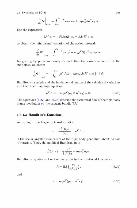
6.6.4.3 Hamilton’s Equations
According to the Legendre transformation,
π =∂L(R,ω)
∂ω= aTJaω
is the scalar angular momentum of the rigid body pendulum about its axisof rotation. Thus, the modified Hamiltonian is
H(R, π) =1
2
π2
aTJa−mgeT3 Rρ0.
Hamilton’s equations of motion are given by the rotational kinematics
R = RS( πa
aTJa
), (6.29)
and
π = mgaT (ρ0 ×RT e3). (6.30)
302 6 Lagrangian and Hamiltonian Dynamics on SO(3)
The Hamiltonian dynamics of the rigid body planar pendulum, characterizedby equations (6.29) and (6.30), are described by the evolution of (R, π) onthe cotangent bundle T ∗M .
6.6.4.4 Reduced Equations for the Rigid Body Planar Pendulum
As we have shown, each material point in the rigid body rotates along a planarcircular arc about a center on the axis of the revolute joint. In particular,the center of mass vector ρ0 rotates along a planar circular arc, with centerat the origin of the inertial frame. The two-dimensional plane containingeach such circular arc is inertially fixed and orthogonal to the axis a ∈ S2.This suggests that it should be possible to describe such rotations in terms ofplanar rotations in S1 as discussed previously in Chapter 4. This connection isclarified in the following development, where the rigid body planar pendulumequations are used to obtain reduced equations that evolve on S1.
To this end, define the direction of the position vector of the center ofmass of the rigid body, expressed in the inertial frame:
ζ =Rρ0
‖Rρ0‖ =Rρ0‖ρ0‖ ,
which follows since ‖Rρ0‖ = ‖ρ0‖. Thus, ζ ∈ S2.It is easy to see that the rotational kinematics (6.27) can be used to obtain
ζ = RRT ζ
= RS(ωa)RT ζ
= S(Rωa)ζ
= S(ωa)ζ,
where we have used a matrix identity and the fact that a = Ra.We now construct a Euclidean orthonormal basis for the inertial frame
given by the ordered triple in S2:
a1, a2, a.
Since aT ζ = 0, we can express
ζ = q1a1 + q2a2,
where q = (q1, q2) ∈ S1. Substituting this into the above rotational kinemat-ics, we obtain
q1a1 + q2a2 = ωS(a) {q1a1 + q2a2}= ω {q1a2 − q2a1} .

6.6 Dynamics on SO(3) 303
Consequently,
q1 = −ωq2,
q2 = ωq1.
In vector form, this can be written as
q = ωSq, (6.31)
where S is the constant 2× 2 skew-symmetric matrix used in Chapter 4.We now express the Euler–Lagrange equation (6.28) in a different form.
Consider the expression
−mgaT (ρ0 ×RT e3) = mgaTS(RT e3)ρ0
= mgaTRTS(e3)Rρ0
= mg ‖ρ0‖ aTS(e3)ζ= mg ‖ρ0‖
{aTS(e3)a1q1 + aTS(e3)a2q2
},
where we have used a matrix identity and the fact that Ra = a. The Euler–Lagrange equation can be expressed as
aTJa ω +mg ‖ρ0‖{aTS(e3)a1q1 + aTS(e3)a2q2
}= 0. (6.32)
Thus, the rotational kinematics (6.31) and the Euler–Lagrange equation (6.32)describe the dynamics of the rigid body planar pendulum in terms of(q, ω) ∈ TS1. These are referred to as reduced equations since they describeonly the dynamics of the position vector of the center of mass of the rigidbody in the inertial frame.
Following a similar development, a reduced form for Hamilton’s equationscan be obtained that describe the evolution on the cotangent bundle T∗M .These results require introduction of the reduced Lagrangian, expressed onthe tangent bundle TS1, definition of the conjugate momentum using theLegendre transformation, and derivation of the reduced Hamilton’s equationson T∗S1. These details are not given here.
6.6.4.5 Conservation Properties
The Hamiltonian, which coincides with the total energy E in this case, isconserved. This can be expressed as
H =1
2aTJaω2 −mgeT3 Rρ0,
which is constant along each solution of the dynamical flow of the rigid bodyplanar pendulum.

304 6 Lagrangian and Hamiltonian Dynamics on SO(3)
6.6.4.6 Equilibrium Properties
The equilibrium or constant solutions of the rigid body planar pendulumoccur when the angular velocity ω = 0 and the rigid body attitude satisfiesthe algebraic equations on the configuration manifold M :
mgaT (ρ0 ×RT e3) = 0,
which implies that the time derivative of the angular velocity vanishes. Thisrequires that the direction of gravity, expressed in the body-fixed frame, andthe center of mass vector ρ0 be collinear.
6.7 Problems
6.1. In this problem, we derive an alternative expression of the momentcaused by an attitude-dependent potential, summarized in Proposition 6.1.
(a) Consider two matrices A,B ∈ R3×3. Let ai, bi ∈ R
3 be the i-th column ofAT and BT for i ∈ {1, 2, 3}, respectively, such that the matrices A andB are partitioned into
A =
⎡⎣a
T1
aT2aT3
⎤⎦ , B =
⎡⎣b
T1
bT2bT3
⎤⎦ .
Show that
BTA−ATB =
3∑i=1
biaTi − aib
Ti =
3∑i=1
S(ai × bi).
(b) Using the above identify, show that the moment caused by an attitude-dependent potential can be rewritten as
−3∑
i=1
ri × ∂L(R,ω)
∂ri=
(RT ∂L(R,ω)
∂R− ∂L(R,ω)
∂R
T
R
)∨
,
where ∂L(R,ω)∂R ∈ R
3×3 is defined such that its i, j-th element corresponds tothe derivative of L(R,ω) with respect to the i, j-th element of R for i, j ∈{1, 2, 3}.6.2. Consider the attitude dynamics of a rigid body described in Section 6.3.3.Here, we rederive the Euler–Lagrange equation given in (6.8) to include the ef-fects of an external moment according to the Lagrange–d’Alembert principle.
6.7 Problems 305
Suppose that there exists an external moment M ∈ R3 acting on the rigid
body. Assume it is resolved in the body-fixed frame.
(a) Let ρ ∈ R3 be the vector from the mass center of the rigid body to a mass
element dm(ρ). Let dF (ρ) ∈ R3 be the force acting on dm(ρ). Assume
that both of ρ and dF (ρ) are expressed in the body-fixed frame. As thereis no external force,
∫B dF (ρ) = 0. Due to the external moment, we have∫
B ρ×dF (ρ) = M . Show that the virtual work due to the external momentis given by
δW =
∫BRdF (ρ) · δRρ =
∫Bη · (ρ× dF (ρ)) = η ·M,
where δR = Rη for η ∈ R3.
(b) From the Lagrange–d’Alembert principle, show that the Euler–Lagrangeequation is given by
Jω + S(ω)Jω −3∑
i=1
S(ri)∂U(R)
∂ri= M.
6.3. Consider the dynamics of a rotating rigid body that is constrained toplanar rotational motion in R
2. That is, the configuration manifold is takenas the Lie group of 2× 2 orthogonal matrices with determinant +1, namelySO(2). The rotational kinematics, expressed in terms of the rotational motiont → R ∈ SO(2), are given by
R = RSω,
for some scalar angular velocity t → ω ∈ R1; as before, S is the standard
2× 2 skew-symmetric matrix. The modified Lagrangian function is given by
L(R,ω) =1
2Jω2 − U(R),
where J is the scalar moment of inertia of the rigid body and U(R) is theconfiguration dependent potential energy function.
(a) What are expressions for the infinitesimal variations of R ∈ SO(2), R ∈TRSO(2), and ω ∈ R
1?(b) Use Hamilton’s principle to derive the Euler equations for the planar
rotations of the rigid body.(c) Use the Legendre transformation to derive Hamilton’s equations for the
planar rotations of the rigid body.(d) What are conserved quantities of the dynamical flow on TSO(2)?(e) What are conditions that define equilibrium solutions of the dynamical
flow on TSO(2)?

306 6 Lagrangian and Hamiltonian Dynamics on SO(3)
6.4. Consider a planar pendulum, with scalar moment of inertia J , underconstant, uniform gravity. Assume the configuration manifold of the planarpendulum is taken to be the Lie group SO(2). Use the results in the priorproblem for the following.
(a) What are the Euler equations for the planar pendulum on the tangentbundle TSO(2)?
(b) What are Hamilton’s equations for the planar pendulum on the cotangentbundle T∗SO(2)?
(c) What are the conserved quantities of the dynamical flow on TSO(2)?(d) What are the equilibrium solutions of the dynamical flow on TSO(2)?
6.5. Consider a double planar pendulum under constant, uniform gravity.The first link rotates about an inertially fixed one degree of freedom revolutejoint. The two links are connected by another revolute joint fixed in the twolinks, constraining the two links to rotate in a common vertical plane. Thescalar moments of inertia of the two pendulums are J1 and J2 about thetwo joint axes. Assume the configuration manifold of the planar pendulumis taken to be the Lie group product (SO(2))2. Use the results in the priorproblem for the following.
(a) What are the Euler–Lagrange equations for the double planar pendulum
on the tangent bundle T (SO(2))2?(b) What are Hamilton’s equations for the double planar pendulum on the
cotangent bundle T∗ (SO(2))2?(c) What are the conserved quantities of the dynamical flow on T (SO(2))2?
(d) What are the equilibrium solutions of the dynamical flow on T (SO(2))2?
6.6. Consider the rigid body planar pendulum considered in subsection 6.6.4.The configuration manifold is M = {R ∈ SO(3) : Ra = a}.(a) Show that the configuration manifold M , which is a submanifold of the
Lie group SO(3), is a one-dimensional matrix Lie group.(b) Show that the configuration manifold M is diffeomorphic to SO(2).
6.7. Consider the free rotational motion of a symmetric rigid body in R3.
Assume the moment of inertia in the body-fixed frame is J = JsI3×3, whereJs > 0 is a scalar.
(a) What are the Euler equations for the free rotational motion of a symmetricrigid body?
(b) Given initial conditions ω(t0) = ω0 ∈ R3, R(t0) = R0 ∈ SO(3), determine
analytical expressions for the angular velocity and for the rigid bodyattitude, the latter described using exponential matrices.
6.8. Consider the free rotational motion of an asymmetric rigid body in R3.
Assume the body-fixed frame is selected so that the moment of inertia isJ = diag(J1, J2, J3), where Ji > 0, i = 1, 2, 3, are distinct.

6.7 Problems 307
(a) What are the Euler equations for the free rotational motion of an asym-metric rigid body?
(b) What are the equilibrium solutions for the dynamical flow defined by theEuler equations? These equilibrium solutions of the Euler equations canbe viewed as relative equilibrium solutions for the complete rotationaldynamics of the asymmetric rigid body.
(c) For each equilibrium solution of the Euler equations, describe the timedependence of the resulting rigid body attitude in SO(3).
6.9. Consider the free rotational motion of a rigid body, with an axis ofsymmetry, in R
3. Assume the body-fixed frame is selected so that the momentof inertia is J = diag(J1, J1, J2), where Ji > 0, i = 1, 2, are distinct.
(a) What are the Euler equations for the free rotational motion of a rigidbody with an axis of symmetry?
(b) What are the equilibrium solutions for dynamical flow defined by theEuler equations? These equilibrium solutions of the Euler equations canbe viewed as relative equilibrium solutions for the complete rotationaldynamics of the rigid body with an axis of symmetry.
(c) For each equilibrium solution of the Euler equations, describe the timedependence of the resulting rigid body attitude in SO(3).
6.10. Consider the rotational motion of a rigid body in R3. Let b ∈ B ⊂ R
3
denote the location of a material point in the body, expressed in the body-fixed frame.
(a) Assume an external force F ∈ R3, expressed in the inertial frame, acts
on the rigid body at the single point in the rigid body denoted by b ∈ B.Show that the component of the force RTF ∈ R
3 in the direction b ∈ Bdoes not influence the rotational dynamics of the rigid body.
(b) What are the Euler equations for the rotational motion of a rigid body,expressed in terms of the external force acting on the rigid body in theinertial frame?
(c) Assume an external force F ∈ R3, expressed in the body-fixed frame, acts
on the rigid body at the single point in the rigid body denoted by b ∈ B.Show that the component of the force F ∈ R
3 in the direction b ∈ B doesnot influence the rotational dynamics of the rigid body.
(d) What are the Euler equations for the rotational motion of a rigid body,expressed in terms of the external force acting on the rigid body in thebody-fixed frame?
6.11. Consider the dynamics of a rigid body, consisting of material pointsdenoted by B in a body-fixed frame, under the influence of a gravitationalfield. The configuration R ∈ SO(3) denotes the attitude of the rigid body.Assume the origin of the body-fixed frame is located at the center of mass ofthe rigid body. A gravitational force acts on each material point in the rigidbody. The net moment of all of the gravity forces is obtained by integrating

308 6 Lagrangian and Hamiltonian Dynamics on SO(3)
the gravity moment for each mass increment of the body over the wholebody. The gravitational field, expressed in the inertial frame, is given byG : R
3 → TR3. The incremental gravitational moment vector on a massincrement dm(ρ) of the rigid body, located at ρ ∈ B in the body-fixed frame,is given in the inertial frame by Rρ × dm(ρ)G(Rρ) or, equivalently in thebody-fixed frame, by ρ× dm(ρ)RTG(Rρ). Thus, the net gravity moment, inthe body-fixed frame, is
∫B ρ×RTG(Rρ) dm(ρ).
(a) What are the Euler equations for the rotational dynamics of the rigidbody in the gravitational field?
(b) What are Hamilton’s equations for the rotational dynamics of the rigidbody in the gravitational field?
(c) What are the conditions for an equilibrium solution of a rotating rigidbody in the gravitational field?
(d) Suppose the gravitational field G(x) = −ge3 is constant. What are thesimplified Euler equations for the rotational dynamics of the rigid body?What are the conditions for an equilibrium solution of a rotating rigidbody in a constant gravitational field?
6.12. Consider the dynamics of a charged rigid body, consisting of materialpoints denoted by B in a body-fixed frame, under the influence of an electricfield and a magnetic field. The configuration R ∈ SO(3) denotes the attitudeof the rigid body. Assume the origin of the body-fixed frame is located atthe center of mass of the rigid body. An electric force and a magnetic forceact on each material point in the rigid body. The net moment of all of theelectric and magnetic forces is obtained by integrating the incremental elec-tric and magnetic moments for each volume increment of the body over thewhole body. The electric field, expressed in the inertial frame, is given byE : R3 → TR3; the magnetic field, expressed in the inertial frame, is givenby B : R3 → TR3 The incremental electric and magnetic moment vectoron a volume increment with charge dQ, located at ρ ∈ B in the body-fixedframe, is given in the inertial frame by Rρ × dQ(E(Rρ) + Rρ × B(Rρ)) or,equivalently in the body-fixed frame, by ρ × dQRT (E(Rρ) + Rρ × B(Rρ)).Thus, the total electric and magnetic moment, in the body-fixed frame, is∫B ρ×RT (E(Rρ) + Rρ×B(Rρ)) dQ.
(a) What are the Euler equations for the rotational dynamics of the rigidbody in the electric field and the magnetic field?
(b) What are Hamilton’s equations for the rotational dynamics of the rigidbody in the electric field and the magnetic field?
(c) What are the conditions for an equilibrium solution of a rotating rigidbody in the electric and the magnetic field?
(d) Suppose the electric field E(x) = −Ee3 and the magnetic field B(x) =Be2 are constant, where E and B are scalar constants. What are thesimplified Euler equations for the rotational dynamics of the rigid body?

6.7 Problems 309
What are the conditions for an equilibrium solution of a rotating rigidbody in this constant electric and magnetic field?
6.13. Consider the rotational motion of a rigid body in R3 acted on by a
force F ∈ R3. The Euler equations are
Jω + ω × Jω = r × F.
In the body-fixed frame, r =∑3
i=1 aiei is a constant vector and F =∑3i=1 fiR
T ei is the force. These are expressed in terms of scalar constantsai, fi, i = 1, 2, 3.
(a) Show that the moment vector is constant in the inertial frame.(b) What are conditions on the constants ai, fi, i = 1, 2, 3 that guarantee
that the Euler equations have an equilibrium solution?(c) What are conditions on the constants ai, fi, i = 1, 2, 3 that guarantee
that the rigid body dynamical flow on TSO(3) has an equilibrium solution(R,ω) = (I3×3, 0) ∈ TSO(3)? Are there other equilibrium solutions in thiscase? What are they?
6.14. Consider the rotational motion of a rigid body in R3 acted on by a
moment vector that is constant in the body-fixed frame. The Euler equationsare
Jω + ω × Jω = M,
where M =∑3
i=1 aiei is the constant moment vector for scalar constantsai, i = 1, 2, 3.
(a) Confirm that the moment vector is constant in the body-fixed frame.(b) Assume the rigid body is asymmetric so that the moment of inertia matrix
J = diag(J1, J2, J3) with distinct entries. Obtain algebraic equations thatcharacterize when the Euler equations have relative equilibrium solutions;that is, the angular velocity vector is constant.
6.15. Consider two concentric rigid spherical shells with common inertiallyfixed centers. The shells, viewed as rigid bodies, are free to rotate subject toa potential that depends only on the relative attitude of the two sphericalshells. The configuration manifold is (SO(3))2 and the modified Lagrangianfunction L : T(SO(3))2 → R
1 is given by
L(R1, R1, ω1, ω2) =1
2ωT1 J1ω1 +
1
2ωT2 J2ω2 −Ktrace(RT
1 R2 − I3×3),
where (Ri, ωi), i = 1, 2, denote the attitudes and angular velocity vectorsof the two spherical shells and J1, J2 are 3 × 3 inertia matrices of the twospherical shells and K is an elastic constant.

310 6 Lagrangian and Hamiltonian Dynamics on SO(3)
(a) What are the Euler–Lagrange equations for the two concentric shells on
the tangent bundle T (SO(3))2?(b) What are Hamilton’s equations for the two concentric shells on the cotan-
gent bundle T∗ (SO(3))2?(c) What are the conserved quantities of the dynamical flow on T (SO(3))2?
(d) What are the equilibrium solutions of the dynamical flow on T (SO(3))2?(e) Determine the linearization that approximates the dynamical flow in a
neighborhood of a selected equilibrium solution.
6.16. It can be shown that the problem of finding the geodesic curves on theLie group SO(3) is equivalent to the problem of finding smooth curves on
SO(3) that minimize∫ 1
0‖ω‖2 dt and connect two fixed points in SO(3).
(a) Using curves described on the interval [0, 1] by t → R(t) ∈ SO(3), show
that geodesic curves satisfy the variational property δ∫ 1
0‖ω‖2 dt = 0 for
all smooth curves t → R(t) ∈ SO(3) that satisfy the boundary conditionsR(0) = R0 ∈ SO(3), R(1) = R1 ∈ SO(3).
(b) What are the Euler–Lagrange equations and Hamilton’s equations thatgeodesic curves on SO(3) must satisfy?
(c) Use the equations and boundary conditions for the geodesic curves todescribe the geodesic curves on SO(3).
6.17. Consider the problem of finding the geodesic curves on the Lie group
SO(3) that minimize∫ 1
0ωTJω dt and connect two fixed points in SO(3). Here
J is a symmetric, positive-definite 3× 3 matrix that is not a scalar multipleof the identity I3×3.
(a) Using curves described on the interval [0, 1] by t → R(t) ∈ SO(3), show
that geodesic curves satisfy the variational property δ∫ 1
0ωTJω dt = 0 for
all smooth curves t → R(t) ∈ SO(3) that satisfy the boundary conditionsR(0) = R0 ∈ SO(3), R(1) = R1 ∈ SO(3).
(b) What are the Euler–Lagrange equations and Hamilton’s equations thatsuch geodesic curves on SO(3) must satisfy?
(c) Describe the impediments in obtaining an analytical expression for suchgeodesics on SO(3).
6.18. Consider n rotating rigid bodies that are coupled through the potentialenergy; the configuration manifold is (SO(3))n. With respect to a commoninertial Euclidean frame, the attitudes of the rigid bodies are given by Ri ∈SO(3), i = 1, . . . , n, and we use the notation R = (R1, . . . , Rn) ∈ (SO(3))n;similarly, ω = (ω1, . . . , ωn) ∈ (R3)n. Suppose the kinetic energy of the rigidbodies is a quadratic function in the angular velocities of the bodies, so thatthe modified Lagrangian function L : T(SO(3))n → R
1 is given by
L(R,ω) =1
2
n∑i=1
ωTi Jiωi +
n∑i=1
aTi ωi − U(R),

6.7 Problems 311
where Ji are 3 × 3 symmetric and positive-definite matrices, i = 1, . . . , n,ai ∈ R
3, i = 1, . . . , n, and U : (SO(3))n → R1 is the potential energy that
characterizes the coupling of the rigid bodies.
(a) What are the Euler–Lagrange equations for this modified Lagrangian forn coupled rigid bodies?
(b) What are Hamilton’s equations for the modified Hamiltonian associatedwith this modified Lagrangian for n coupled rigid bodies?


![[M. G. Calkin] Lagrangian and Hamiltonian Mechanic(BookZZ.org)](https://static.fdocuments.in/doc/165x107/563db7ff550346aa9a8f97ff/m-g-calkin-lagrangian-and-hamiltonian-mechanicbookzzorg.jpg)
