Chapter 6 Inheritance and Gift Taxation

Lectures on Public Finance Part 2_Chap 6, 2016 version P.1 of 23 Last updated 12/4/2016

Chapter 6 Inheritance and Gift Taxation

6.1 Introduction1 Death taxes may be imposed for a variety of reasons. One of them, on which this paper focuses,

is redistribution. The institution of inheritance is a major factor responsible for concentration of

wealth and, indirectly, for income inequality. According to most recent estimates, inherited wealth

accounts for almost half of the net worth of households2. Death taxes, especially in the form of

inheritance taxation, can thus (at least potentially) be used to moderate economic inequalities.

There are, however, more subtle effects of death taxation that might be significant; they are

stressed by those who are less enthusiastic about such taxation. In addition to the alleged reduction

of savings, there is the concern that death taxation may adversely affect equality. According to

Becker (1974, 1991) and Tomes (1981), transfers between generations follow a ‘regression towards

the mean’ mechanism with bequests and gifts flowing from well-to-do donors to less well-to-do

recipients. Within each family, transfers thus tend to offset inequalities. Where this is true,

taxation will mitigate the redistributive effect of wealth transfers.

The question one might raise at this point is why the government couldn’t directly effect the

appropriate redistribution across and within generations. In a perfect information setting, it is clear

that taxes on wealth transfers could be tuned in such a way that redistribution within families is not

discouraged while redistribution across families is fostered. In an asymmetric information setting,

however, this is less clear. Well to do families could be induced to leave lower bequests to avoid a

too heavy tax burden; at the same time, the government could not be able to implement the ‘right’

redistribution because of imperfect information as to wealth holding.

It should be pointed out that the government can affect bequest behavior not only through the tax

schedule, but also through the choice of the tax base or even through restrictions on estate sharing.

Polar cases include estate taxes (based on the total amount which is bequeathed) and inheritance

taxes (based on individual shares) or even accession taxes (based on individual shares plus other

resources). Because tax schedules are typically non-linear (and progressive) the definition of the

tax base is of crucial importance. In addition, bequests are subject to a variety of legal rules

including more or less stringent equal sharing rules (amongst children).

1 Section 1-3 draw heavily from Cremer and Pestieau (2001) 2 For a survey of empirical studies on bequests, see Arrondel et al. (1997).


6.2 Optimal Inheritance Tax with Bequests in the Utility

6.2.1 Model3

We consider a dynamic economy with a discrete set of generations 0, 1, …, t , … and no growth.

Each generation has measure 1, lives one period, and is replaced by the next generation. Individual ti (from dynasty i living in generation t ) receives pre-tax inheritance 0≥tib from generation

1−t at the beginning of period t . The initial distribution of bequests ib0 is exogenously given.

Inheritances earn an exogenous gross rate of return R per generation. We relax the no-growth

and small open economy fixed factor price assumptions at the end of Section 6.2.3.

Individual Maximization Individual ti has exogenous pre-tax wage rate tiw , drawn from an arbitrary but stationary

ergodic distribution (with potential correlation of individual draws across generations). Individual ti works til , and earns titiLti lwy = at the end of period and then splits lifetime resources (the

sum of net-of-tax labor income and capitalized bequests received) into consumption tic and

bequests left 01 ≥+ itb . We assume that there is a linear labor tax at rate Ltτ , a linear tax on

capitalized bequests at rate Btτ , and a lump-sum grant tE 4. Individual ti has utility function

),,( lbcV ti increasing in consumption ticc = and net-of-tax capitalized bequests left

)1( 11 ++ −= BtitRbb τ , and decreasing in labor supply till = . Like tiw , preferences tiV are

also drawn from an arbitrary ergodic distribution. Hence, individual ti solves

)),1(,max 110,, 1tiBtitti

ti

bcllRbcV

ittiti++≥

−+

τ s.t. (1)

tLttitiBttiitti ElwRbbc +−+−=+ + )1()1(1 ττ .

The individual first order condition for bequests left itb 1+ is tibBt

tic VRV )1( 1+−= τ if 01 >+ itb .

Equilibrium Definition

3 This part is drawn heavily from Piketty and Saez (2013, pp.1853-73). 4 Note that Btτ taxes both the raw bequest received tib and the lifetime return to bequest tibR ⋅− )1( , so it

should really be interpreted as a broad-based capital tax rather than as a narrow inheritance tax.


We denote by Lttt ycb ,, aggregate bequests received, consumption, and labor income in

generation t . We assume that the stochastic processes for utility functions tiV and for wage

rates tiw are such that, with constant tax rates and lump-sum grant, the economy converges to a

unique ergodic steady-state equilibrium independent of the initial distribution of bequests iib )( 0 .

All we need to assume is an ergodicity condition for the stochastic process for tiV and tiw .

Whatever parental taste and ability, one can always draw any other taste or productivity.5 In

equilibrium, all individuals maximize utility as in (1) and there is a resulting steady-state ergodic equilibrium distribution of bequests and earnings ),( 0iLti yb . In the long run, the position of each

dynasty i is independent of the initial position ),( 00 iLi yb .

6.2.2 Stesdy-State Welfare Maximization

For pedagogical reasons, we start with the case where the government considers the long-run

steady-state equilibrium of the economy and chooses steady-state long-run policy BLE ττ ,, to maximize steady-state social welfare, defined as a weighted sum of individual utilities with Pareto weights 0≥tiω , subject to a period-by-period budget balance

LtLtB yRbE ττ += :

)),1(,)1()1((max 11, tiBititLtitiBtii

titi lRbbElRbVSWF

BL

ττωτωττ

−−+−+−= ++∫ . (2)

In the ergodic equilibrium, social welfare is constant over time. Taking the lump-sum grant E as fixed, Lτ and Bτ are linked to meet the budget constraint, LtLtB yRbE ττ += . As we shall

see, the optimal Bτ depends on the size of behavioral responses to taxation captured by elasticities,

and the combination of social preferences and the distribution of bequests and earnings captured by

distributional parameters, which we introduce in turn.

Elasticity Parameters The aggregate variable tb is a function of Bτ−1 (assuming that Lτ adjusts), and Lty is a

function of Lτ−1 (assuming that Bτ adjusts). Formally, we can define the corresponding

long-run elasticities as

5 See Piketty and Saez (2012) for a precise mathematical statement and concrete examples. Ramdom taste shocks

can generate Pareto distributions with realistic levels of wealth concentration – which are difficult to generate with labor productivity shocks alone. Random shocks to rates of return would work as well.


. )1(

1

and )1(

1 :

EL

Lt

Lt

LL

EB

t

t

BB

ddy

ye

ddb

beesElasticitirunLong

ττ

ττ

−+

−=

−+

−=−

(3)

That is, Be is the long-run elasticity of aggregate bequest flow (i.e., aggregate capital

accumulation) with respect to the net-of-bequest-tax rate Bτ−1 , while Le is the long-run

elasticity of aggregate labor supply with respect to the net-of-labor-tax rate Lτ−1 . Importantly,

those elasticities are policy elasticities (Hendren (2013)) that capture responses to a joint and budget

neutral change ),( LB ττ . Hence, they incorporate both own- and cross-price effects. Empirically,

Le and Be can be estimated directly using budget neutral joint changes in ),( BL ττ or indirectly

by decomposing Le and Be into own- and cross-price elasticities, and estimating these

separately.

Distributional Parameters

We denote by )tjctjj

tictiti VVg ωω ∫= the social marginal welfare weight on individual ti .

The weights tig are normalized to sum to 1. tig measures the social value of increasing

consumption of individual ti by $1 (relative to distributing the $1 equally across al individuals).

Under standard redistributive preferences, tig is low for the well-off (those with high bequests

received or high earnings) and high for the worse-off. To capture distributional parameters of

earnings, bequests received, bequests left, we use the ratios – denoted with an upper bar – of the population average weighted by social marginal welfare weights tig to the unweighted population

average (recall that the tig weights sum to 1). Formally, we have

.

, , : and 1

1leftreceived

Lt

i Ltiti

L

t

i itti

t

i titi

y

ygy

b

bgb

b

bgbParametersonalDistributi

∫

∫∫

=

==+

+

(4)

Each of those ratios is below 1 if the variable is lower for those with high social marginal welfare

weights. With standard redistributive preferences, the more concentrated the variable is among the

well-off, the lower the distributional parameter.


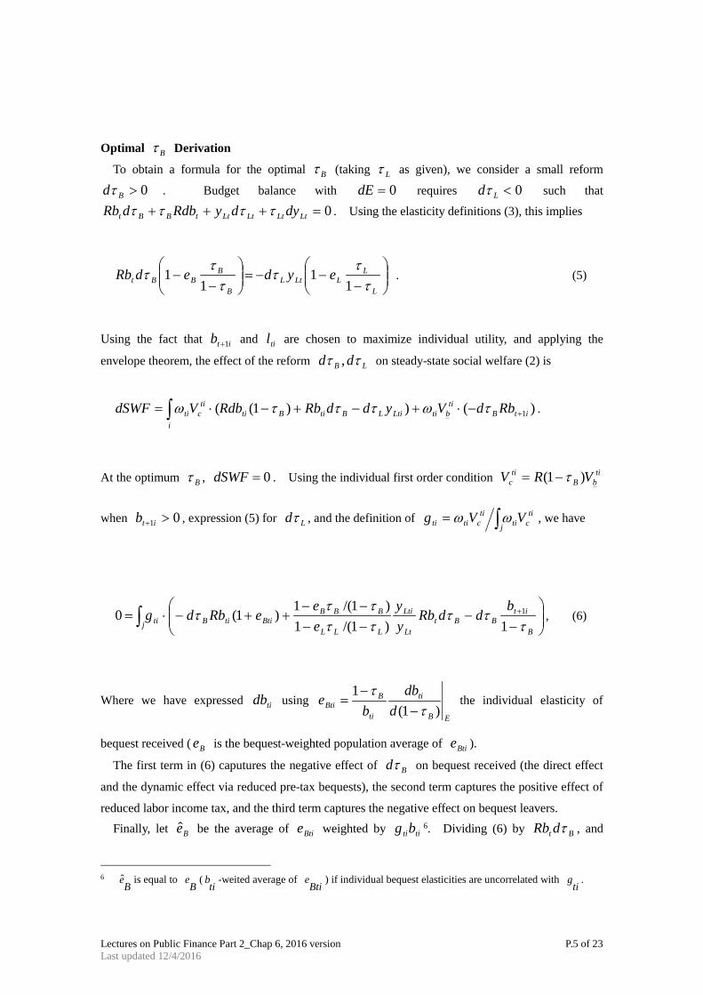
Optimal Bτ Derivation

To obtain a formula for the optimal Bτ (taking Lτ as given), we consider a small reform

0>Bdτ . Budget balance with 0=dE requires 0<Ldτ such that

0=+++ LtLtLtLttBBt dydyRdbdRb ττττ . Using the elasticity definitions (3), this implies

−

−−=

−

−L

LLLtL

B

BBBt eydedRb

ττ

ττ

ττ

11

11 . (5)

Using the fact that itb 1+ and til are chosen to maximize individual utility, and applying the

envelope theorem, the effect of the reform LB dd ττ , on steady-state social welfare (2) is

)())1(( 1itBti

btiLtiLBtiBtii

ticti RbdVyddRbRdbVdSWF +−⋅+−+−⋅= ∫ τωτττω .

At the optimum Bτ , 0=dSWF . Using the individual first order condition tibB

tic VRV )1( τ−=

when 01 >+ itb , expression (5) for Ldτ , and the definition of ∫=j

ticti

tictiti VVg ωω , we have

−

−−−−−

++−⋅= +∫B

itBBt

Lt

Lti

LLL

BBBBtitiBj ti

bddRb

yy

ee

eRbdgτ

ττττττ

τ1)1/(1

)1/(1)1(0 1 , (6)

Where we have expressed tidb using EB

ti

ti

BBti d

dbb

e)1(

1τ

τ−

−= the individual elasticity of

bequest received ( Be is the bequest-weighted population average of Btie ).

The first term in (6) caputures the negative effect of Bdτ on bequest received (the direct effect

and the dynamic effect via reduced pre-tax bequests), the second term captures the positive effect of

reduced labor income tax, and the third term captures the negative effect on bequest leavers. Finally, let Be be the average of Btie weighted by titibg 6. Dividing (6) by Bt dRb τ , and

6

Be is equal to

Be (

tib -weited average of

Btie ) if individual bequest elasticities are uncorrelated with

tig .


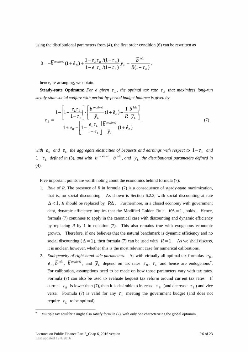
using the distributional parameters from (4), the first order condition (6) can be rewritten as

)1()1/(1)1/(1

)ˆ1(0left

received

BL

LLL

BBBB R

byee

ebτττ

ττ−

−−−−−

++−= ,

hence, re-arranging, we obtain.

Steady-state Optimum: For a given Lτ , the optimal tax rate Bτ that maximizes long-run

steady-state social welfare with period-by-period budget balance is given by

)ˆ1(1

11

1)ˆ1(1

11

received

leftreceived

BLL

LLB

LB

LL

LL

B

ey

bee

yb

Re

ybe

+

−

−−+

++⋅

−

−−=

ττ

ττ

τ , (7)

with Be and Le the aggregate elasticities of bequests and earnings with respect to Bτ−1 and

Lτ−1 defined in (3), and with receivedb , leftb , and Ly the distributional parameters defined in

(4).

Five important points are worth noting about the economics behind formula (7):

1. Role of R. The presence of R in formula (7) is a consequence of steady-state maximization,

that is, no social discounting. As shown is Section 6.2.3, with social discounting at rate

1<∆ , R should be replaced by ∆R . Furthermore, in a closed economy with government

debt, dynamic efficiency implies that the Modified Golden Rule, 1=∆R , holds. Hence,

formula (7) continues to apply in the canonical case with discounting and dynamic efficiency

by replacing R by 1 in equation (7). This also remains true with exogenous economic

growth. Therefore, if one believes that the natural benchmark is dynamic efficiency and no

social discounting ( 1=∆ ), then formula (7) can be used with 1=R . As we shall discuss,

it is unclear, however, whether this is the most relevant case for numerical calibrations.

2. Endogeneity of right-hand-side parameters. As with virtually all optimal tax formulas Be ,

Le , leftb , receivedb , and Ly depend on tax rates Bτ , Lτ and hence are endogenous7.

For calibration, assumptions need to be made on how those parameters vary with tax rates.

Formula (7) can also be used to evaluate bequest tax reform around current tax rates. If

current Bτ is lower than (7), then it is desirable to increase Bτ (and decrease Lτ ) and vice

versa. Formula (7) is valid for any Lτ meeting the government budget (and does not

require Lτ to be optimal).

7 Multiple tax equilibria might also satisfy formula (7), with only one characterizing the global optimum.


3. Comparative statics. Bτ decreases with the elasticity Be for standard efficiency reasons

and increases with Le as a higher earnings elasticity makes it more desirable to increase Bτ

to reduce Lτ . Bτ naturally decreases with the distributional parameters receivedb and leftb , that is, the social weight put on bequests receivers and leavers. Under a standard

utilitarian criterion with decreasing marginal utility of disposable income, welfare weights

tig are low when bequests and/or earnings are high. As bequests are more concentrated

than earnings (Piketty (2011)), we expect Lyb <received and Lyb <left . When bequests

are infinitely concentrated, Lybb <<leftreceived , and (7) boils down to )1/(1 BB e+=τ , the revenue maximizing rate. Conversely, when the tig ’s put weight on large inheritors,

then 1received >b and Bτ can be negative.

4. Pros and cons of taxing bequests. Bequest taxation differs from capital taxation in a

standard OLG model with no bequests in two ways. First, Bτ hurts both donors ( leftb

effect) and donees ( receivedb effect), making bequests taxation relatively less desirable. Second, bequests introduce a new dimension of lifetime resources inequality, lowering

Lyb /received , Lyb /left and making bequests taxation more desirable. This intuition is

made precise in Section 6.2.4 where we specialize our model to the Farhi-Werning two-period

case with uni-dimensional inequality.

5. General soccial marginal welfare weights. General social marginal welfare weights allow

great flexibility in the social welfare criterion choice (Saez and Stantcheva (2013)). One

normatively appealing concept is that individuals should be compensated for inequality they

are not responsible for – such as bequests received – but not for inequality they are

responsible for – such as labor income (Fleurbaey (2008)). This amounts to setting social welfare weights tig to zero for all bequest receivers and setting them positive and uniform

on zero-bequests receivers. About half the population in France or the United States

receives negligible bequests. Hence, this “Meritocratic Rawlsian” optimum has broader

appeal than the standard Rawlsian case.

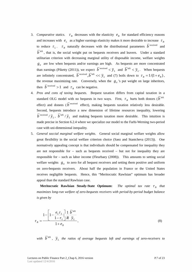
Meritocratic Rawlsian Steady-State Optimum: The optimal tax rate Bτ that

maximizes long-run welfare of zero-bequests receivers with period-by-period budget balance

is given by

B

LL

LL

B ey

bR

e

+

−

−−=

1

11

11left

ττ

τ , (8)

with leftb , Ly the ratios of average bequests left and earnings of zero-receivers to


population averages.

In that case, even when zero-receivers have average labor earnings (i.e., 1=Ly ), if

bequests are quantitatively important in lifetime resources, zero-receivers will leave smaller

bequests than average, so that 1left <b . Formula (8) then implies 0>Bτ even with

1=R and 0=Le .

In the inelastic labor case, formula (8) further simplifies to B

LB e

yRb+

−=

1)(1 left

τ . If we

further assume 0=Be and 1=R (benchmark case with dynamic efficiency and 1=∆ ),

the optimal tax rate L

B yb left

1−=τ depends only on distributional parameters, namely the

relative position of zero-bequest receivers in the distributions of bequests left and labor

income. For instance, if %50left =Lyb , for example, zero-bequest receivers expect to

leave bequests that are only half of average bequest and to receive average labor income, then

it is in their interest to tax bequests at rate %50=Bτ . Intuitively, with a 50% bequest tax

rate, the distortion on the “bequest left” margin is so large that the utility value of one

additional dollar devoted to bequests is twice larger than one additional dollar devoted to

consumption. For the same reasons, if %100left =Lyb , but 2=R , then %50=Bτ .

If the return to capital doubles the value of bequests left at each generation, then it is in the

interest of zero-receivers to tax capitalized bequest at a 50% rate, even if they plan to leave as

many bequests as the average. These intuitions illustrate the critical importance of

distributional parameters – and also of perceptions. If everybody expects to leave large

bequests, then subjectively optimal Bτ will be fairly small – or even negative.

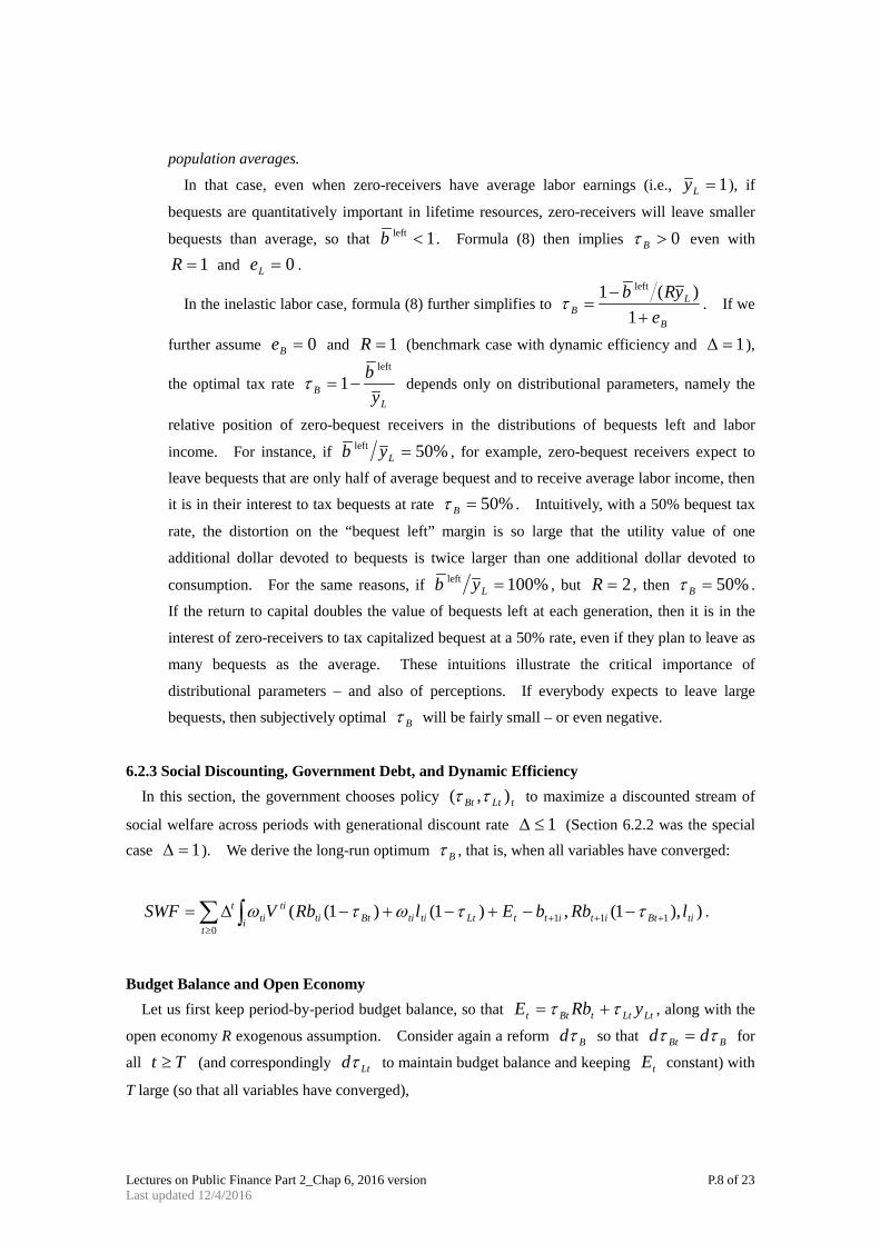
6.2.3 Social Discounting, Government Debt, and Dynamic Efficiency In this section, the government chooses policy tLtBt ),( ττ to maximize a discounted stream of

social welfare across periods with generational discount rate 1≤∆ (Section 6.2.2 was the special case 1=∆ ). We derive the long-run optimum Bτ , that is, when all variables have converged:

)),1(,)1()1(( 1110

tiBtitittLttitiBttiti

i tit

t lRbbElRbVSWF +++≥

−−+−+−∆= ∫∑ ττωτω .

Budget Balance and Open Economy Let us first keep period-by-period budget balance, so that LtLttBtt yRbE ττ += , along with the

open economy R exogenous assumption. Consider again a reform Bdτ so that BBt dd ττ = for

all Tt ≥ (and correspondingly Ltdτ to maintain budget balance and keeping tE constant) with

T large (so that all variables have converged),


).(

))1((

11

itBti

bi tiTt

t

LtiLtBtiBtiti

ci tiTt

t

RbdV

yddRbRdbVdSWF

+−≥

≥

−⋅∆+

−−−⋅∆=

∫∑

∫∑τω

τττω

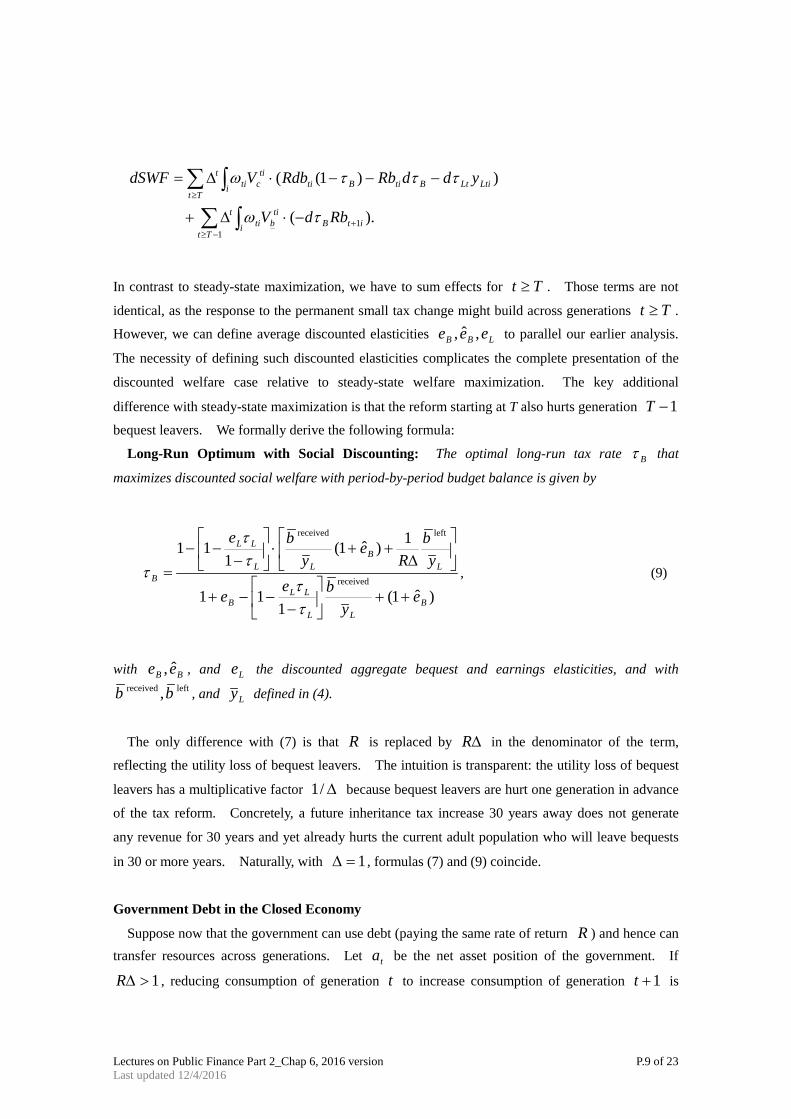
In contrast to steady-state maximization, we have to sum effects for Tt ≥ . Those terms are not

identical, as the response to the permanent small tax change might build across generations Tt ≥ .

However, we can define average discounted elasticities LBB eee ,ˆ, to parallel our earlier analysis.

The necessity of defining such discounted elasticities complicates the complete presentation of the

discounted welfare case relative to steady-state welfare maximization. The key additional

difference with steady-state maximization is that the reform starting at T also hurts generation 1−T

bequest leavers. We formally derive the following formula:

Long-Run Optimum with Social Discounting: The optimal long-run tax rate Bτ that

maximizes discounted social welfare with period-by-period budget balance is given by

)ˆ1(1

11

1)ˆ1(1

11

received

leftreceived

BLL

LLB

LB

LL

LL

B

ey

bee

yb

Re

ybe

++

−

−−+

∆

++⋅

−

−−=

ττ

ττ

τ , (9)

with BB ee ˆ, , and Le the discounted aggregate bequest and earnings elasticities, and with leftreceived ,bb , and Ly defined in (4).

The only difference with (7) is that R is replaced by ∆R in the denominator of the term,

reflecting the utility loss of bequest leavers. The intuition is transparent: the utility loss of bequest

leavers has a multiplicative factor ∆/1 because bequest leavers are hurt one generation in advance

of the tax reform. Concretely, a future inheritance tax increase 30 years away does not generate

any revenue for 30 years and yet already hurts the current adult population who will leave bequests

in 30 or more years. Naturally, with 1=∆ , formulas (7) and (9) coincide.

Government Debt in the Closed Economy

Suppose now that the government can use debt (paying the same rate of return R ) and hence can transfer resources across generations. Let ta be the net asset position of the government. If

1>∆R , reducing consumption of generation t to increase consumption of generation 1+t is


desirable (and vice versa). Hence, if 1>∆R , the government wants to accumulate infinite assets.

If 1<∆R , the government wants to accumulate infinite debts. In both cases, the small open

economy assumption would cease to hold. Hence, a steady-state equilibrium only exists if the

Modified Golden Rule 1=∆R holds.

Therefore, it is natural to consider the closed-economy case with endogenous capital stock

ttt abK += , CRS production function ),( tt LKF , where tL is the total labor supply, and

where rates of returns on capital and labor are given by Kt FR += 1 and Lt Fw = . Denoting by

)1( Bttt RR τ−= and )1( Lttt ww τ−= the after-tax factor prices, the government budget

dynamics is given by tttttttttt ELwwbRRaRa −−+−+=+ )()(1 . Two results can be

obtained I that context.

First, going back or an instant to the budget balance case, it is straight-forward to show that formla

(9) carries over unchanged in this case. This is a consequence of the standard optimal tax result of

Diamond and Mirrlees (1971) that optimal tax formulas are the same with fixed prices and

endogenous prices. The important point is that the elasticities Be and Le are pure supply

elasticities (i.e., keeping factor prices constant). Intuitively, the government chooses the net-of-tax prices tR and tw and the resource constraint is tttttttt ELwbRLbFb −−−+= ),(0 , so that

the pre-tax factors effectively drop out of the maximization problem and the same proof goes

through (see the Supplemental Material (Piketty and Saez (2013b)) for complete details). Second,

and most important, moving to the case with debt, we can show that the long-run optimum takes the

following form.

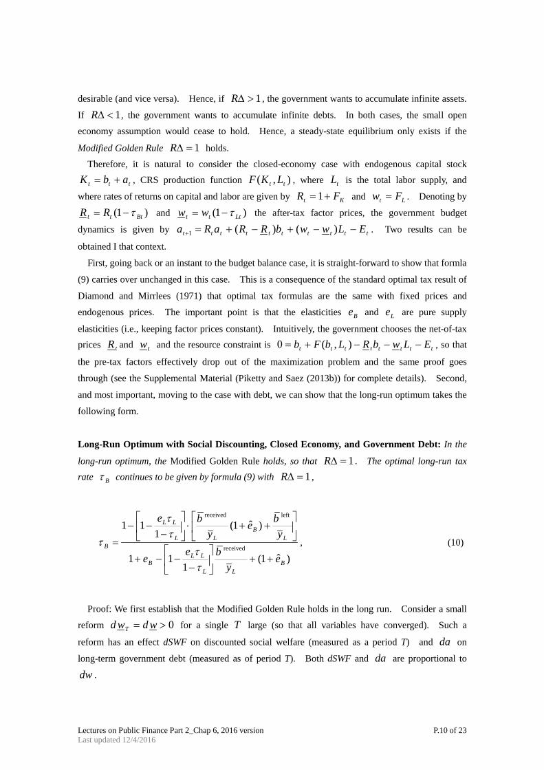
Long-Run Optimum with Social Discounting, Closed Economy, and Government Debt: In the

long-run optimum, the Modified Golden Rule holds, so that 1=∆R . The optimal long-run tax rate Bτ continues to be given by formula (9) with 1=∆R ,

)ˆ1(1

11

)ˆ1(1

11

received

leftreceived

BLL

LLB

LB

LL

LL

B

ey

bee

ybe

ybe

++

−

−−+

++⋅

−

−−=

ττ

ττ

τ , (10)

Proof: We first establish that the Modified Golden Rule holds in the long run. Consider a small

reform 0>= wdwd T for a single T large (so that all variables have converged). Such a

reform has an effect dSWF on discounted social welfare (measured as a period T) and da on

long-term government debt (measured as of period T). Both dSWF and da are proportional to

dw .


Now consider a second reform 01 <=+ wRdwd T at 1+T only. By linearity of small

changes, this reform has welfare effect dSWFRdSWF ∆−=' , as it is R− times larger and

happens one period after the first reform. The effect on government debt is Rdada −='

measured as of period 1+T , and hence da− measured as of period T (i.e., the same absolute

effect as the initial reform). Hence, the sum of the two reforms would be neutral for government

debt. Therefore, if social welfare is maximized, the sum has to be neutral from a social welfare

perspective as well, implying that 0'=+ dSWFdSWF so that 1=∆R .

Next, we can easily extend the result above that the optimal tax formula takes the same form with

endogenous factor prices. Hence, (9) applies with 1=∆R . Q.E.D.

This result shows that dynamic efficiency considerations (i.e., optimal capital accumulation) are

conceptually orthogonal to cross-sectional redistribution considerations. That is, whether or not

dynamic efficiency prevails, there are distributional reasons pushing for inheritance taxation, as well

as distortionary effects pushing in the other direction, resulting in an equity-efficiency trade-off that

is largely independent from aggregate capital accumulation issues8.

One natural benchmark would be to assume that we are at the Modified Golden Rule (though this

is not necessarily realistic). In that case, the optimal tax formula (10) is independent of R and

∆ and depends solely on elasticities LB ee , and the distributional factors leftreceived ,bb , Ly .

If the Modified Golden Rule does not hold (which is probably more plausible) and there is too

little capital, so that 1>∆R , then the welfare cost of taxing bequests left is smaller and the optimal

tax rate on bequests should be higher (everything else being equal). The intuition for this result is

simple: if 1>∆R , pushing resources toward the future is desirable. Taxing bequests more in

period T hurts period 1−T bequest leavers and befits period T labor earners, effectively

creating a transfer from period 1−T toward period T . This result and intuition depend on our

assumption that bequests left by generation 1−t are taxed in period t as part of generation t

lifetime resources. This fits with actual practice, as bequest taxes are paid by definition at the end

of the lives of bequest leavers and paid roughly in the middle of the adult life of bequest receivers9. If we assume instead that period t taxes are LtLttBt yb ττ ++1 , then formula (9) would have no

∆R term dividing leftb , but all the terms in receivedb would be multiplied by ∆R . Hence, in

the Meritocratic Rawlsian optimum where 0received =b , we can obtain (10) by considering steady-state maximization subject to tLtLttBt Eyb =++ ττ 1 and without the need to consider

dynamic efficiency issues.

The key point of this discussion is that, with government debt and dynamic efficiency ( 1=∆R ),

formula (10) no longer depends on the timing of tax payments. 8 The same decoupling results have been proved in the OLG model with only life-cycle savings with linear Ramsey

taxation and a representative agent per generation (King (1980), Atkinson and Sandmo (1980)). 9 Piketty and Saez (2012) made this point formally with a continuum of overlapping cohorts. With accounting

budget balance, increasing bequest taxes today allows to reduce labor taxes today, hurting the old who are leaving bequests and benefiting current younger labor earners (it is too late to reduce the labor taxes of the old).


Economic Growth

Normatively, there is no good justification for discounting the welfare of future generations, that is,

for assuming 1<∆ . However, with 1=∆ , the Modified Golden Rule implies that 1=R so

that the capital stock should be infinite. A standard way to eliminate this unappealing result as well

as making the model more realistic is to consider standard labor augmenting economic growth at rate

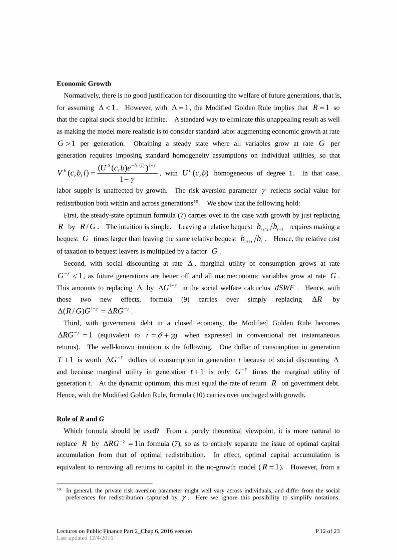
1>G per generation. Obtaining a steady state where all variables grow at rate G per

generation requires imposing standard homogeneity assumptions on individual utilities, so that

γ

γ

−=

−−

1)),((),,(

1)(lhtiti

tiebcUlbcV , with ),( bcU ti homogeneous of degree 1. In that case,

labor supply is unaffected by growth. The risk aversion parameter γ reflects social value for

redistribution both within and across generations10. We show that the following hold:

First, the steady-state optimum formula (7) carries over in the case with growth by just replacing R by GR / . The intuition is simple. Leaving a relative bequest 11 ++ tit bb requires making a

bequest G times larger than leaving the same relative bequest tit bb 1+ . Hence, the relative cost

of taxation to bequest leavers is multiplied by a factor G .

Second, with social discounting at rate ∆ , marginal utility of consumption grows at rate

1<−γG , as future generations are better off and all macroeconomic variables grow at rate G .

This amounts to replacing ∆ by γ−∆ 1G in the social welfare calcuclus dSWF . Hence, with those two new effects, formula (9) carries over simply replacing R∆ by

γγ −− ∆=∆ RGGGR 1)/( .

Third, with government debt in a closed economy, the Modified Golden Rule becomes

1=∆ −γRG (equivalent to gr γδ += when expressed in conventional net instantaneous

returns). The well-known intuition is the following. One dollar of consumption in generation

1+T is worth γ−∆G dollars of consumption in generation t because of social discounting ∆

and because marginal utility in generation 1+t is only γ−G times the marginal utility of generation t. At the dynamic optimum, this must equal the rate of return R on government debt.

Hence, with the Modified Golden Rule, formula (10) carries over unchaged with growth.

Role of R and G

Which formula should be used? From a purely theoretical viewpoint, it is more natural to

replace R by 1=∆ −γRG in formula (7), so as to entirely separate the issue of optimal capital accumulation from that of optimal redistribution. In effect, optimal capital accumulation is

equivalent to removing all returns to capital in the no-growth model ( 1=R ). However, from a

10 In general, the private risk aversion parameter might well vary across individuals, and differ from the social

preferences for redistribution captured by γ . Here we ignore this possibility to simplify notations.


practical policy viewpoint, it is probably more justified to replace R by GR / in formula (7) and

to use observed R and G to calibrate the formula. The issue of optimal capital accumulation is

very complex, and there are many good reasons why the Modified Golden Rule 1=∆ −γRG does not seem to be followed in the real world. In practice, it is very difficult to know what the optimal

level of capital accumulation really is. Maybe partly as a consequence, governments tend not to

interfere too massively with the aggregate capital accumulation process and usually choose to let

private forces deal with this complex issue (net government assets – positive or negative – are

typically much smaller than net private assets). One pragmatic viewpoint is to take these reasons as

given and impose period-by-period budget constraint (so that the government does not interfere at all

with aggregate capital accumulation), and consider steady-state maximization, in which case we

obtain formula (7) with GR / .

Importantly, the return rate R and the growth rate G matter for optimal inheritance rates even

in the case with dynamic efficiency. A larger GR / implies a higher level of aggregate bequest

flows (Piketty (2011)), and also a higher concentration of inherited wealth. Therefore, a larger

GR / leads to smaller receivedb and leftb and hence a higher Bτ .

6.2.4 Role of Bi-Dimensional Inequality: Contrast With Farhi-Werning

Our results on positive inheritance taxation (under specific redistributive social criteria) hinge

crucially on the fact that, with inheritances, labor income is no longer a complete measure of lifetime

resources, that is, our model has bi-dimensional (labor income, inheritance) inequality.

To see this, consider the two-period mode of Farhi and Werning (2010), where each dynasty lasts

for two generations with working parents starting with no bequests and children receiving bequests

and never working. In this model, all parents have the same utility function, hence earnings and

bequests are perfectly correlated so that inequality is uni-dimensional (and solely due to the earnings

ability of the parent). This model can be nested within the class of economies we have considered

by simply assuming that each dynasty is a succession of (non-overlapping) two-period-long

parent-child pairs, where children have zero wage rates and zero taste for bequests. Formally,

preferences of parents have the form ),,( lbcV P , while preferences of children have the simpler

form )(cV C . Because children are totally passive and just consume the net-of-tax bequests they

receive, parents’ utility functions are de facto altruistic (i.e., depend on the utility of the child) in this

model 11 . In general equilibrium, the parents and children are in equal proportion in any

cross-section. Assuming dynamic efficiency 1=∆R , our previous formula (10) naturally applies

11 This assumes that children do not receive the lump-sum grant tE (that accrues only to parents). Lump-sum

grants to children can be considered as well and eliminated without loss of generality if parents’ preferences are altruistic and hence take into account the lump-sum grant their children get ,that is, the parents’ utility is

),)1(,( 111 tichildtBtitti

ti lERbcV +++ +−τ . Farhi and Werning (2010) considered this altruistic case.


to this specific model.

Farhi and Werning (2010) analyzed the general case with nonlinear taxation with weakly

separable parents’ utilities of the form )),,(( lbcuU i . If social welfare puts weight only on

parents (the utility of children is taken into account only through the utility of their altruistic parents),

the Atkinson-Stiglitz theorem applies and the optimal inheritance tax rate is zero. If social welfare

puts additional direct weight on children, then the inheritance tax is less desirable and the optimal

tax rate becomes naturally negative12. We can obtain the linear tax counterpart of these results if

we further assume that the sub-utility ),( bcu is homogeneous of degree 1. This assumption is

needed to obtain the linear tax version of Atkinson-Stiglitz (Deaton (1979)).

Optimal Bequest Tax in the Farhi-Werning Version of Our Model: In the parent-child model

with utilities of parents such that )),,((),,( lbcuUlbcV titi = with ),( bcu homogeneous of

degree 1 and homogeneous in the population and with dynamic efficiency ( 1=∆R ): If the social welfare function puts zero direct weight o children, then 0=Bτ is optimal.

If the social welfare function puts positive direct weight on children, then 0<Bτ is optimal.

The proof is in Piketty and Saez (2013a), where we show that any tax system ),,( ELB ττ can be

replaced by a tax system )',',0'( ELB ττ = that leaves all parents as well off and raises more

revenue. The intuition can be understood using our optimal formula (10). Suppose for simplicity

here that there is no lump-sum grant. With ),( bcu homogeneous, bequest decisions are linear in

lifetime resources so that )1(1 LtLtiit ysb τ−⋅=+ , where s is homogeneous in the population.

This immediately implies that LtLtiti

ctititti

cti yyVEbbVE /][/][ 11 ωω =++ so that Lyb =left .

Absent any behavioral response, bequest taxes are equivalent to labor taxes on distributional grounds

because there is only one dimension of inequality left. Next, the bequest tax Bτ also reduces

labor supply (as it reduces the use of income) exactly in the same proportion as the labor tax.

Hence, shifting from the labor tax to the bequest tax has zero net effect on labor supply and

0=Le . As parents are the zero-receivers in this model, we have 0received =b when social

welfare counts only parents’ welfare. Therefore, optimal tax formula (10) with Ltyb =left and

0=Le implies that 0<Bτ . If children (i.e., bequest receivers) also enter social welfare, then

0received >b . In that case, formula (10) with Ltyb =left and 0=Le implies that 0<Bτ .

As our analysis makes clear, however, the Farhi-Werning (2010) two-period model only provides

an incomplete characterization of the bequest tax problem because it fails to capture the fact that

lifetime resources inequality is bi-dimensional, that is, individuals both earn and receive bequests.

12 Farhi and WErning (2010) also obtained valuable results on the progressivity of the optimal bequest tax subsidy

that cannot be captured in our linear framework.


This key bi-dimensional feature makes positive bequest taxes desirable under some redistributive

social welfare criteria. An extension to our general model would be to consider nonlinear (but

static) earnings taxation. The Atkinson-Stiglitz zero tax result would no longer apply as,

conditional on labor earnings, bequests left are a signal for bequests received, and hence correlated

with social marginal welfare weights, violating Assumption 1 of Saez’s (2002) extension of

Atkinson-Stiglitz to heterogeneous populations. The simplest way to see this is to consider the case

with uniform labor earnings: Inequality arises solely from bequests, labor taxation is useless for

redistribution, and bequest taxation is the only redistributive tool.

6.2.5 Accidental Bequests or Wealth Lovers

Individuals also leave bequests for non-altruistic reasons. For example, some individuals may

value wealth per se (e.g., it brings social prestige and power), or for precautionary motives, and

leave accidental bequests due to imperfect annuitization. Such non-altruistic reasons are

quantitatively important (Kopczuk and Lupton (2007)). If individuals do not care about the

after-tax bequests they leave, they are not hurt by bequest taxes on bequests they leave. Bequest

receivers continue to be hurt by bequest taxes. This implies that the last term leftb in the numerator of our formulas, capturing the negative effect of Bτ on bequest leavers, ought to be

discounted. Formally, it is straightforward to generalize the model to utility functions

),,,(ti lbbcV , where b is pre-tax bequest left, which captures wealth loving motives. The

individual first order condition becomes tib

tibBt

tic VVRV +−= + )1( 1τ and

tic

tibBtti VVRv /)1( 1+−= τ naturally captures the relative importance of altruism in bequests

motives. All our formulas carry over by simply replacing leftb by leftbv ⋅ , with v the population average of tiv (weighted by ittibg 1+ ). Existing surveys can be used to measure the

relative importance of altruistic motives versus other motives to calibrate the optimal Bτ . Hence,

our approach is robust and flexible to accommodate such wealth loving effects that are empirically

first order.

6.3 Optimal Inheritance Tax in the Dynastic Model

6.3.1 The Dynastic Model

The Barro-Becker dynastic model has been widely used in the analysis of optimal

capital/inheritance taxation. Our sufficient statistics formula approach can also fruitfully be used in

that case, with minor modifications. In the dynastic model, individuals care about the utility of


their heirs itV 1+ instead of the after-tax capitalized bequests itBt bR 11 )1( ++−τ they leave. The

standard assumption is the recursive additive form ittiti VlcuV 1),( ++= δ , where 1<δ is a

uniform discount factor. We assume again a linear and deterministic tax policy 0),,( ≥ttLtBt Eττ .

Individual ti chooses itb 1+ and til to maximize itttiti

ti VElcu 1),( ++ δ subject to the

individual budget ttitiBttiitti ElwRbbc ++−=+ + )1(1 τ with 01 ≥+ itb , where ittVE 1+ denotes

expected utility of individual it 1+ (based on information known in period t ). The first order

condition for itb 1+ implies the Euler equation itctBt

tic uERu 1

1)1( ++−= τδ (whenever 01 >+ itb ).

With stochastic ergodic processes for wages tiw and preferences tiu , standard regularity

assumptions, this model also generates an ergodic equilibrium where long-run individual outcomes

are independent of initial position. Assuming again that the tax policy converges to ),,( EBL ττ ,

the long-run aggregate bequests and earnings Ltt yb , also converge and depend on asymptotic tax

rates BL ττ , . We show in Piketty and Saez (2013a) that this model generates finite long-run

elasticities LB ee , defined as in (3) that satisfy (5) as in Section 6.2. The long-run elasticity Be

becomes infinite when stochastic shocks vanish. Importantly, as itb 1+ is known at the end of

period t , the individual first order condition in itb 1+ implies that (regardless of whether

01 =+ itb ):

][)1( 1111

itcittBtit

tic ubERbu +

+++ −=⋅ τδ and hence ,)1(received

11left

1 +++ −= tBtt bRb τδ (11)

with ticiit

titicii

tubbu

b0

0received

ωω∫

∫= and ti

ciit

itticii

tub

bub

01

10left1

ωω∫

∫=

+

++ as in (4) for any dynastic Pareto weights

ii )( 0ω . Paralleling the analysis of Section 6.2, we start with steady-state welfare maximization in Section

6.3.2 and then consider discounted utility maximization in Section 6.3.3.

6.3.2 Optimum Long-Run Bτ in Steady-State Welfare Maximization

We start with the utilitarian case (uniform Pareto weights 10 ≡iω ). We assume that the

economy is in steady-state ergodic equilibrium with constant tax policy ELB ,,ττ set such that the

government budget constraint EyRb LtLtB =+ττ holds each period. As in Section 6.2.2, the


government chooses Bτ (with Lτ adjusting to meet the budget constraint and with E

exogenously given) to maximize discounted steady-state utility:

)])1()1(([max 10

tiitLtitiBtiti

t

t lbElwRbuEEVB

+≥

∞ −+−+−= ∑ ττδτ

,

where we assume (w.l.o.g.) that the steady state has been reached in period 0. ib0 is given to the

individual (but depends on Bτ ), while tib for 1≥t and til for 0≥t are chosen optimally so

that the envelope theorem applies. Therefore, first order condition with respect to Bτ is

],[][ ][])1([0

01

1

0

10

00

0

LLtitic

t

tBit

itc

t

tBi

iciB

ic

dyuEdRbuEdRbuEdbRuE

τδτδ

ττ

⋅−⋅−

⋅−−⋅=

∑∑≥

++

≥

+

where we have broken out into two terms the effect of Bdτ . Using (5) linking Ldτ to, Bdτ ,

)1(1 0

0 B

i

i

BBi d

dbb

eτ

τ−

−= , and the individual first order condition

itit

ctBittic buERbu 1

11 )1( +

++ −= τδ ,

∑≥

+

−−−−

+−

−++−=0

10

0

)1/(1)1/(1

1][

)]1([0t Lt

Lti

LLL

BBBt

tic

B

ittict

Biii

c yy

ee

RbuEbuE

eRbuEττττ

τδ . (12)

The sum in (12) is a repeat of identical terms because the economy is in ergodic steady state.

Hence, the only difference with (6) in Section 6.2 is that the second and third terms are repeated

(with discount factor δ ), hence multiplied by )1/(11 2 δδδ −=+++ . Hence, this is

equivalent to discounting the first term (bequest received effect) by a factor δ−1 , so that we only

need to replace receivedb by received)1( bδ− in formula (7). Hence, conditional on elasticities

and distributional parameters, the dynastic case makes the optimal Bτ larger because double

counting costs of taxation are reduced relative to the bequests in the utility model of Section 6.2.


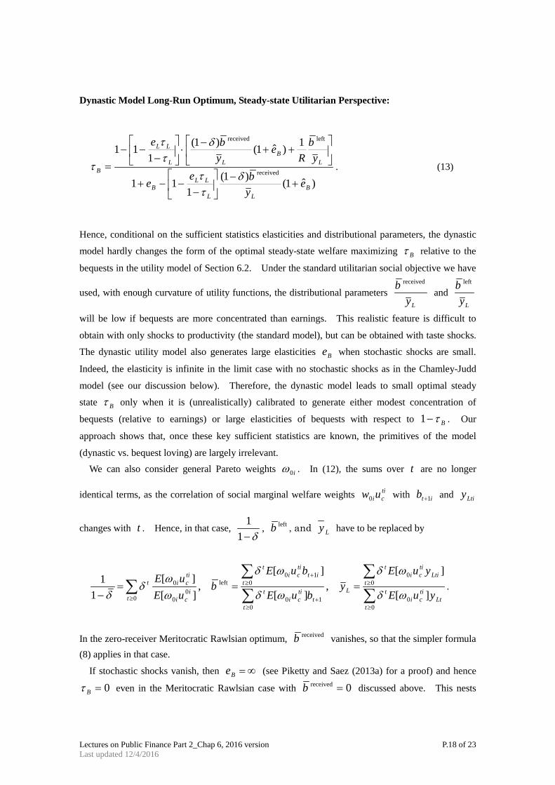
Dynastic Model Long-Run Optimum, Steady-state Utilitarian Perspective:

)ˆ1()1(1

11

1)ˆ1()1(1

11

received

leftreceived

BLL

LLB

LB

LL

LL

B

eybee

yb

Re

ybe

+−

−

−−+

++

−⋅

−

−−=

δττ

δττ

τ . (13)

Hence, conditional on the sufficient statistics elasticities and distributional parameters, the dynastic

model hardly changes the form of the optimal steady-state welfare maximizing Bτ relative to the

bequests in the utility model of Section 6.2. Under the standard utilitarian social objective we have

used, with enough curvature of utility functions, the distributional parameters Ly

b received

and Ly

b left

will be low if bequests are more concentrated than earnings. This realistic feature is difficult to

obtain with only shocks to productivity (the standard model), but can be obtained with taste shocks.

The dynastic utility model also generates large elasticities Be when stochastic shocks are small.

Indeed, the elasticity is infinite in the limit case with no stochastic shocks as in the Chamley-Judd

model (see our discussion below). Therefore, the dynastic model leads to small optimal steady

state Bτ only when it is (unrealistically) calibrated to generate either modest concentration of

bequests (relative to earnings) or large elasticities of bequests with respect to Bτ−1 . Our

approach shows that, once these key sufficient statistics are known, the primitives of the model

(dynastic vs. bequest loving) are largely irrelevant. We can also consider general Pareto weights i0ω . In (12), the sums over t are no longer

identical terms, as the correlation of social marginal welfare weights ticiuw0 with itb 1+ and Ltiy

changes with t . Hence, in that case, δ−1

1, leftb , and Ly have to be replaced by

Lttici

t

t

Ltitici

t

t

Lt

tici

t

t

ittici

t

t

ici

tici

t

t

yuE

yuEy

buE

buEb

uEuE

][

][ ,

][

][ ,

][][

11

00

00

100

100left

00

0

0 ωδ

ωδ

ωδ

ωδ

ωω

δδ ∑

∑∑∑

∑≥

≥

+≥

+≥

≥

===−

.

In the zero-receiver Meritocratic Rawlsian optimum, receivedb vanishes, so that the simpler formula (8) applies in that case.

If stochastic shocks vanish, then ∞=Be (see Piketty and Saez (2013a) for a proof) and hence

0=Bτ even in the Meritocratic Rawlsian case with 0received =b discussed above. This nests


the steady-state maximization version of Chamley and Judd (presented in Piketty (2000, p.444)) that

delivers a zero Bτ optimum when the supply elasticity of capital is infinite even when the

government cares only about workers with zero wealth.

Finally, it is possible to write a fully general model ittiti VlbbcuV 1),,,( ++= δ that

encompasses many possible bequest motivations. The optimal formula in the steady state continues

to take the same general shape we have presented, although notations are more cumbersome.

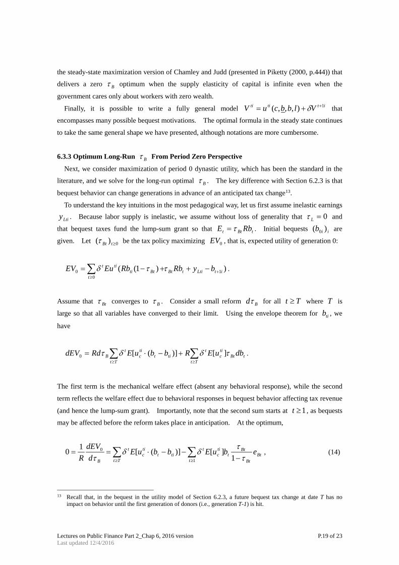
6.3.3 Optimum Long-Run Bτ From Period Zero Perspective

Next, we consider maximization of period 0 dynastic utility, which has been the standard in the

literature, and we solve for the long-run optimal Bτ . The key difference with Section 6.2.3 is that

bequest behavior can change generations in advance of an anticipated tax change13.

To understand the key intuitions in the most pedagogical way, let us first assume inelastic earnings

Ltiy . Because labor supply is inelastic, we assume without loss of generality that 0=Lτ and

that bequest taxes fund the lump-sum grant so that tBtt RbE τ= . Initial bequests iib )( 0 are

given. Let 0)( ≥tBtτ be the tax policy maximizing 0EV , that is, expected utility of generation 0:

))1(( 10

0 itLtitBtt

Bttitit byRbRbEuEV +

≥

−++−= ∑ ττδ .

Assume that Btτ converges to Bτ . Consider a small reform Bdτ for all Tt ≥ where T is

large so that all variables have converged to their limit. Using the envelope theorem for tib , we

have

tTt Tt

Bttic

ttit

tic

tB dbuERbbuERddEV ∑ ∑

≥ ≥

+−⋅= τδδτ ][)]([0 .

The first term is the mechanical welfare effect (absent any behavioral response), while the second

term reflects the welfare effect due to behavioral responses in bequest behavior affecting tax revenue

(and hence the lump-sum grant). Importantly, note that the second sum starts at 1≥t , as bequests

may be affected before the reform takes place in anticipation. At the optimum,

∑ ∑≥ ≥ −

−−⋅==Tt t

BtBt

Btt

tic

ttit

tic

t

B

ebuEbbuEd

dEVR 1

0

1][)]([10

ττ

δδτ

, (14)

13 Recall that, in the bequest in the utility model of Section 6.2.3, a future bequest tax change at date T has no

impact on behavior until the first generation of donors (i.e., generation T-1) is hit.


with )1(

1

B

t

t

tBt d

dbb

Be

ττ

−−

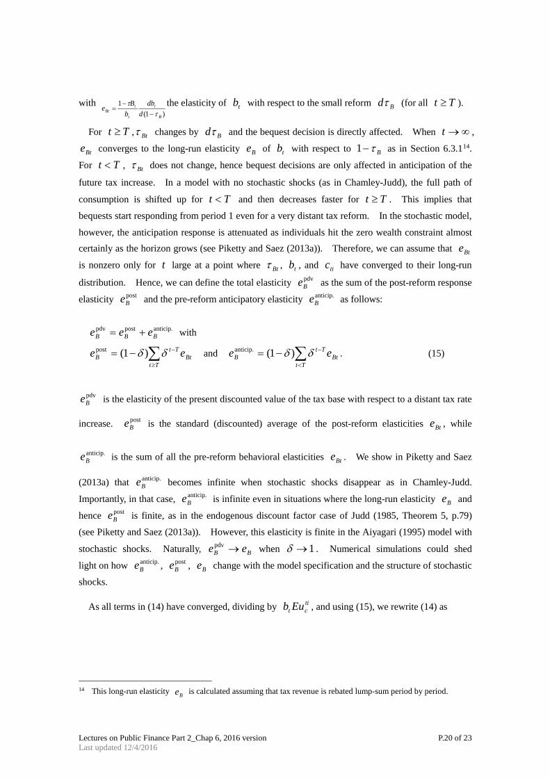
=the elasticity of tb with respect to the small reform Bdτ (for all Tt ≥ ).

For Tt ≥ , Btτ changes by Bdτ and the bequest decision is directly affected. When ∞→t ,

Bte converges to the long-run elasticity Be of tb with respect to Bτ−1 as in Section 6.3.114.

For Tt < , Btτ does not change, hence bequest decisions are only affected in anticipation of the

future tax increase. In a model with no stochastic shocks (as in Chamley-Judd), the full path of

consumption is shifted up for Tt < and then decreases faster for Tt ≥ . This implies that

bequests start responding from period 1 even for a very distant tax reform. In the stochastic model,

however, the anticipation response is attenuated as individuals hit the zero wealth constraint almost certainly as the horizon grows (see Piketty and Saez (2013a)). Therefore, we can assume that Bte

is nonzero only for t large at a point where Btτ , tb , and tic have converged to their long-run

distribution. Hence, we can define the total elasticity pdvBe as the sum of the post-reform response

elasticity postBe and the pre-reform anticipatory elasticity anticip.

Be as follows:

anticip.postpdvBBB eee += with

BtTt

TtB ee ∑

≥

−−= δδ )1(post and BtTt

TtB ee ∑

<

−−= δδ )1(anticip. . (15)

pdvBe is the elasticity of the present discounted value of the tax base with respect to a distant tax rate

increase. postBe is the standard (discounted) average of the post-reform elasticities Bte , while

anticip.Be is the sum of all the pre-reform behavioral elasticities Bte . We show in Piketty and Saez

(2013a) that anticip.Be becomes infinite when stochastic shocks disappear as in Chamley-Judd.

Importantly, in that case, anticip.Be is infinite even in situations where the long-run elasticity Be and

hence postBe is finite, as in the endogenous discount factor case of Judd (1985, Theorem 5, p.79)

(see Piketty and Saez (2013a)). However, this elasticity is finite in the Aiyagari (1995) model with

stochastic shocks. Naturally, BB ee →pdv when 1→δ . Numerical simulations could shed

light on how anticip.Be , post

Be , Be change with the model specification and the structure of stochastic

shocks.

As all terms in (14) have converged, dividing by tict Eub , and using (15), we rewrite (14) as

14 This long-run elasticity Be is calculated assuming that tax revenue is rebated lump-sum period by period.


Btt

t

B

B

ttic

titic

Tt

t ebuE

buE ∑∑≥≥ −

−

−=

11][][

10 δτ

τδ , hence

pdv

1][][

10 BB

Btict

titic euEbbuE

ττ−

−−= .

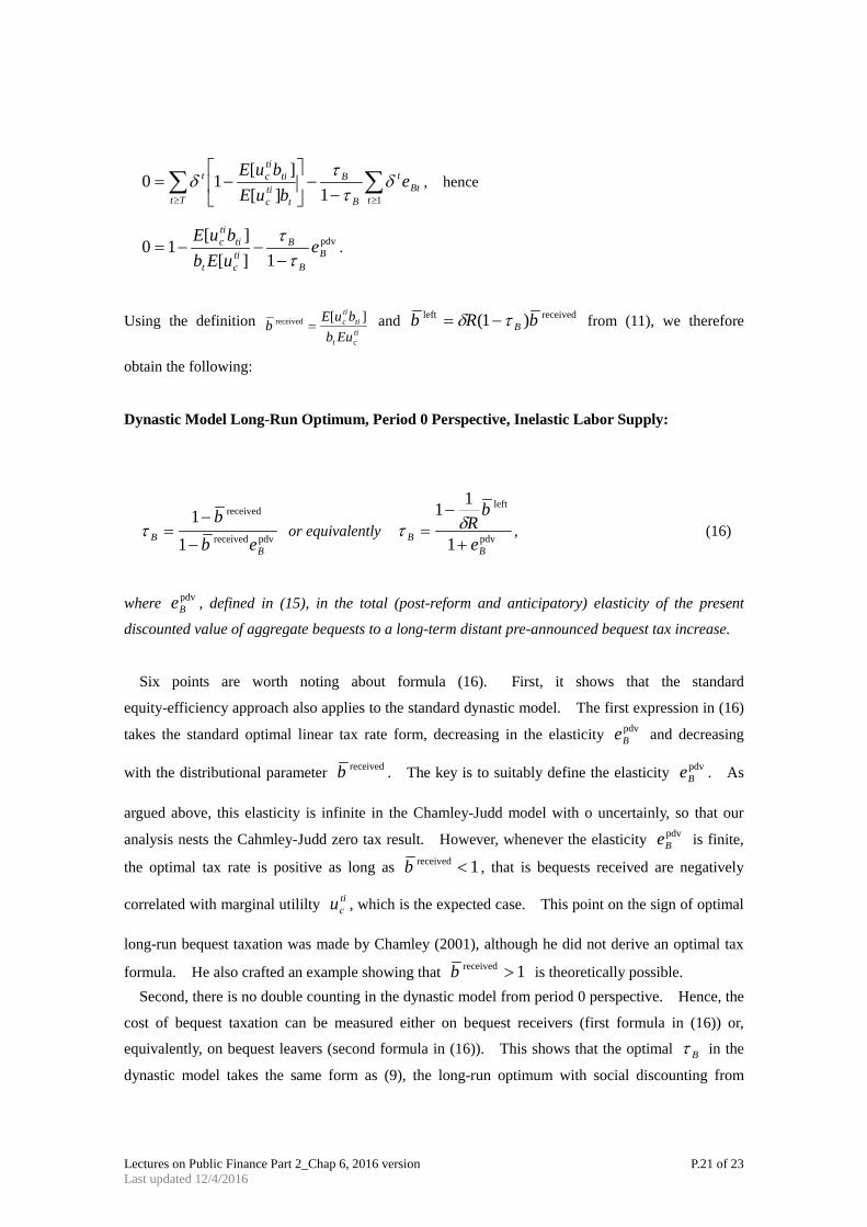
Using the definition tict

titic

EubbuE

b][received = and receivedleft )1( bRb Bτδ −= from (11), we therefore

obtain the following:

Dynastic Model Long-Run Optimum, Period 0 Perspective, Inelastic Labor Supply:

pdvreceived

received

11

BB eb

b−

−=τ or equivalently pdv

left

1

11

BB e

bR

+

−= δτ , (16)

where pdvBe , defined in (15), in the total (post-reform and anticipatory) elasticity of the present

discounted value of aggregate bequests to a long-term distant pre-announced bequest tax increase.

Six points are worth noting about formula (16). First, it shows that the standard

equity-efficiency approach also applies to the standard dynastic model. The first expression in (16)

takes the standard optimal linear tax rate form, decreasing in the elasticity pdvBe and decreasing

with the distributional parameter receivedb . The key is to suitably define the elasticity pdvBe . As

argued above, this elasticity is infinite in the Chamley-Judd model with o uncertainly, so that our

analysis nests the Cahmley-Judd zero tax result. However, whenever the elasticity pdvBe is finite,

the optimal tax rate is positive as long as 1received <b , that is bequests received are negatively

correlated with marginal utililty ticu , which is the expected case. This point on the sign of optimal

long-run bequest taxation was made by Chamley (2001), although he did not derive an optimal tax

formula. He also crafted an example showing that 1received >b is theoretically possible. Second, there is no double counting in the dynastic model from period 0 perspective. Hence, the

cost of bequest taxation can be measured either on bequest receivers (first formula in (16)) or,

equivalently, on bequest leavers (second formula in (16)). This shows that the optimal Bτ in the

dynastic model takes the same form as (9), the long-run optimum with social discounting from


Section 6.2, ignoring the welfare effect on bequest receivers, that is, setting 0received =b .15. Third, we can add labor supply decisions. Considering a Bdτ , Ldτ trade-off modifies the

optimal tax rate as expected. receivedb and leftb in (16) need to be replaced by

−

−L

LL

L

ey

bττ

11

pvdreceived and

−

−L

LL

L

ey

bττ

11

pvdleft , with pdvLe the elasticity of aggregate PDV earnings (see

Section S.1.3).

Fourth, optimal government debt management in the closed economy would deliver the Modified

Golden Rule 1=Rδ and the same formulas continue to hold (see Section S.1.4). Fifth, we can consider heterogeneous discount rate tiδ . Formula (16) still applies with

ttictiiTt

titictiiTt

T buEbuE

b][

][lim

1

1received

δδδδ

≥

≥

∑∑

= . Hence, receivedb puts weight on consistently altruistic

dynasties, precisely those that accumulate wealth so that 1received >b and 0<Bτ is likely. In

that case, the period 0 criterion puts no weight on individuals who had non-altruistic ancestors.

This fits with aristocratic values, but is the polar opposite of realistic modern meritocratic values.

Hence, the dynastic model with the period zero objective generates unappealing normative

recommendations when there is heterogeneity in tastes for bequests. Sixth, adding Pareto weights i0ω that depend on initial position delivers exactly the same

formula, as the long-run position of each individual is independent of the initial situation. This

severely limits the scope of social welfare criteria in the period 0 perspective model relative to the

steady-state welfare maximization model analyzed in Section 6.3.2.

15 Naturally, 0== LL eτ here. Note also that Ly is replaced by 1 because the trade-off here is between the

bequest tax and the lump-sum grant (instead of the labor tax as in Section 6.2).


References

Abel, A., G. Mankiw, L. Summers, and R. Zeckhauser (1989) “Assessing dynamic efficiency:

Theory an devidence.” Review of Economic Studies, 56: 1-20. Atkinson, A., and A. Sandmo (1980) “Welfare implications of the taxation of savings.”

Economic Journal, 90: 529-49. Auerbach, A., and L. Kotlikoff (1987) Dynamic Fiscal Policy, Cambridge University Press. Blumkin T. and E. Sadka (2003) “Estate taxation with intended and accidental bequests.”

Journal of Public Economics, 88: 1-21. Chamley, C. (1986) “Optimal taxation of capital income in general equilibrium with infinite

lives.” Econometrica, 54: 607-22. Chamley, C. (2001) “Capital income taxation, wealth distribution and borrowing constraints.”

Journal of Public Economics, 79: 55-69. Cremer H. and P. Pestieau (2001) “Non-linear taxation of bequests, equal sharing rules and the

tradeoff between intra- and inter-family inequalities.” Journal of Public Economics, 79: 35-53.

Diamond, P. (1965) “National debt in a neoclassical growth model.” American Economic Review, 55:1126-50.

Gordon, R. (1986) “Taxation of investment and savings in a world economy.” American Economic Review, 76: 1086-1102.

Hilman, A.L. (2003) Public Finance and Public Policy, Cambridge; Cambridge University Press.

Judd, K. (1985) “Redistributive taxation in a simple perfect foresight model.” Journal of Public Economics, 28: 59-83.

Krusell, P., L. Ohanian, J.-V. Rios-Rull, and G. Violante (2000) “Capital-skill complementarity and inequality: A macroeconomic analysis.” Econometrica, 68: 1029-53.

Kopczuk, W. (2013) “Taxation of Transfers and Wealth” in Handbook of Public Economics, vol.5, Amsterdam: North-Holland. [1852]

Ordover, J., and E. Phelps (1979) “The concept of optimal taxation in the overlapping generations model of capital and wealth.” Journal of Public Economics, 12: 1-26.

Piketty, T., and E. Saez (2012) “A Theory of Optimal Capital Taxation” Working Paper 17989, NBER. [1854, 1862, 1879 1880]

Piketty, T., and E. Saez (2013a) “A Theory of Optimal Inheritance Taxation” Econometrica, 81(5): 1851-86.

Piketty, T., and E. Saez (2013b) “Supplement to ‘A Theory of Optimal Capital Taxation’, ” Econometrica Supplemental Material, 81, http://www.econometricsociety.org/ecta/supmat/10712_proofs.pdf; http://www.econometricsociety.org/ecta/supmat/10712_programs_and _data.zip. [1861]

Salanié, B. (2003) The Economics of Taxation, Cambridge, MA; The MIT Press Samuelson, P. (1958) “An exact consumption-loan model of interest with or without the social

contrivance of money.” Journal of Political Economy, 66: 467-82. Stiglitz, J. (1985) “Inequality and capital taxation.” IMSSS Technical Report 457, Stanford

University. Summers, L. (1981) “Taxation and capital accumulation in a life cycle growth model.”

American Economic Review, 71: 533-54. Tobin, J. (1958) “Liquidity preference as behavior towards risk.” Review of Economic Studies,

25: 65-8. Tuomala M. (1985) “Uncertain lifetime, life insurance, and the theory of consumer.” Review of

Economic Studies, 32: 137-50.

http://www.econometricsociety.org/ecta/supmat/10712_proofs.pdf

http://www.econometricsociety.org/ecta/supmat/10712_programs_and%20_data.zip

Chapter 6 Inheritance and Gift Taxation

Documents

Transcript of Chapter 6 Inheritance and Gift Taxation