Chapter 6 Finite Differences - Engineering...
18
Chapter 6 Finite Differences 6.1 Introduction For a function = , finite differences refer to changes in values of (dependent variable) for any finite (equal or unequal) variation in (independent variable). In this chapter, we shall study various differencing techniques for equal deviations in values of and associated differencing operators; also their applications will be extended for finding missing values of a data and series summation. 6.2 Shift or Increment Operator () Shift (Increment) operator denoted by ‘’ operates on () as = + Or = + , where ‘’ is the step height for equi-spaced data points. Clearly effect of the shift operator is to shift the function value to the next higher value + or + Also 2 = () = + = +2 ∴ = + Moreover −1 = − , where −1 is the inverse shift operator. 6.3 Differencing Operators If 0 , 1 , 2 , … be the values of for corresponding values of 0 , 1 , 2 , … , then the differences of are defined by ( 1 − 0 ) , ( 2 − 1 ) , … ,( − −1 ) , and are denoted by different operators discussed in this section. 6.3.1 Forward Difference Operator ∆ Forward difference operator ‘∆’ operates on as ∆ = +1 − Or ∆ = + − , where is the height of differencing. ∴ ∆ 0 = 1 − 0 ∆ 1 = 2 − 1 ⋮ ∆ = +1 − Also ∆ 2 0 = ∆ 1 − ∆ 0 = 2 − 1 − 1 − 0 = 2 − 2 1 + 0 ⋮ ∆ 0 = − 1 −1 + 2 −2 −⋯ + −1 −1 −1 1 + −1 0 Generalizing ∆ = + − 1 +−1 + 2 +−2 −⋯ + −1 Here ∆ is the order forward difference; Table 6.1 shows the forward differences of various orders.
Transcript of Chapter 6 Finite Differences - Engineering...

Chapter 6
Finite Differences
6.1 Introduction
For a function 𝑦 = 𝑓 𝑥 , finite differences refer to
changes in values of 𝑦 (dependent variable) for any
finite (equal or unequal) variation in 𝑥 (independent
variable).
In this chapter, we shall study various differencing
techniques for equal deviations in values of 𝑥 and
associated differencing operators; also their
applications will be extended for finding missing
values of a data and series summation.
6.2 Shift or Increment Operator (𝑬)
Shift (Increment) operator denoted by ‘𝐸’ operates on 𝑓(𝑥) as 𝐸𝑓 𝑥 = 𝑓 𝑥 +
Or 𝐸𝑦𝑥 = 𝑦𝑥+ , where ‘’ is the step height for equi-spaced data points.
Clearly effect of the shift operator 𝐸 is to shift the function value to the next
higher value 𝑓 𝑥 + or 𝑦𝑥+
Also 𝐸2𝑓 𝑥 = 𝐸 𝐸𝑓(𝑥) = 𝐸𝑓 𝑥 + = 𝑓 𝑥 + 2
∴ 𝐸𝑛𝑓 𝑥 = 𝑓 𝑥 + 𝑛
Moreover 𝐸−1𝑓 𝑥 = 𝑓 𝑥 − , where 𝐸−1 is the inverse shift operator.
6.3 Differencing Operators
If 𝑦0, 𝑦1, 𝑦2 , …𝑦𝑛 be the values of 𝑦 for corresponding values of 𝑥0, 𝑥1, 𝑥2 ,
…𝑥𝑛 , then the differences of 𝑦 are defined by (𝑦1 − 𝑦0), (𝑦2 − 𝑦1), … , (𝑦𝑛 − 𝑦𝑛−1) , and are denoted by different operators discussed in this section.
6.3.1 Forward Difference Operator ∆
Forward difference operator ‘∆’ operates on 𝑦𝑥 as ∆𝑦𝑥 = 𝑦𝑥+1− 𝑦𝑥
Or ∆𝑓 𝑥 = 𝑓 𝑥 + − 𝑓 𝑥 , where is the height of differencing.
∴ ∆𝑦0 = 𝑦1− 𝑦0
∆𝑦1 = 𝑦2− 𝑦1
⋮
∆𝑦𝑛 = 𝑦𝑛+1− 𝑦𝑛
Also ∆2𝑦0 = ∆𝑦1− ∆𝑦0 = 𝑦2− 𝑦1 − 𝑦1− 𝑦0 = 𝑦2 − 2𝑦1 + 𝑦0
⋮
∆𝑛𝑦0 = 𝑦𝑛 − 𝑛𝐶1𝑦𝑛−1 + 𝑛𝐶2𝑦𝑛−2 −⋯+ −1 𝑛−1 𝑛𝐶𝑛−1𝑦1 + −1 𝑛𝑦0
Generalizing ∆𝑛𝑦𝑟 = 𝑦𝑛+𝑟 − 𝑛𝐶1𝑦𝑛+𝑟−1 + 𝑛𝐶2𝑦𝑛+𝑟−2 −⋯+ −1 𝑟𝑦𝑟
Here ∆𝑛 is the 𝑛𝑡 order forward difference; Table 6.1 shows the forward
differences of various orders.

Table 6.1 Forward Differences
𝒙 𝒚 ∆ ∆𝟐 ∆𝟑 ∆𝟒 ∆𝟓 𝒙𝒐 𝑦𝑜
∆𝑦𝑜 𝒙𝟏 𝑦1 ∆2𝑦𝑜
∆𝑦1 ∆3𝑦𝑜 𝒙𝟐 y2 ∆2𝑦1 ∆4𝑦0
∆𝑦2 ∆3𝑦1 ∆5𝑦0 𝒙𝟑 𝑦3 ∆2𝑦2 ∆4𝑦1
∆𝑦3 ∆3𝑦2 𝒙𝟒 𝑦4 ∆2𝑦3
∆𝑦4 𝒙𝟓 𝑦5
The arrow indicates the direction of differences from top to bottom. Differences in
each column notate difference of two adjoining consecutive entries of the previous
column.
Relation between ∆ and 𝑬
∆ and 𝐸 are connected by the relation ∆ ≡ 𝐸 − 1
Proof: we know that ∆𝑦𝑛 = 𝑦𝑛+1− 𝑦𝑛
= 𝐸𝑦𝑛− 𝑦𝑛
⇒ ∆𝑦𝑛 = 𝐸 − 1 𝑦𝑛
⇒ ∆ ≡ 𝐸 − 1 or 𝐸 ≡ 1 + ∆
Properties of operator ‘∆’
∆𝐶 = 0 , 𝐶 being a constant
∆𝐶 𝑓(𝑥) = 𝐶𝑓(𝑥)
∆[𝑎𝑓 𝑥 ± 𝑏𝑔(𝑥)] = 𝑎 ∆𝑓 𝑥 ± 𝑏 ∆𝑔(𝑥)
∆ 𝑓 𝑥 𝑔 𝑥 = 𝑓 𝑥 + ∆ 𝑔 𝑥 + 𝑔 𝑥 ∆𝑓 𝑥 , 𝑓 & 𝑔 may be interchanged
∆ 𝑓 𝑥
𝑔 𝑥 =
𝑔 𝑥 ∆𝑓 𝑥 −𝑓(𝑥)∆𝑔 𝑥
𝑔 𝑥+ 𝑔 𝑥
Result 1: The 𝒏𝒕𝒉 differences of a polynomial of degree 'n' are constant and all
higher order differences are zero.
Proof: Consider the polynomial 𝑓(𝑥) of 𝑛𝑡 degree
𝑓(𝑥) = 𝑎0𝑥𝑛 + 𝑎1𝑥
𝑛−1 + 𝑎2𝑥𝑛−2 + ⋯+ 𝑎𝑛−1𝑥 + 𝑎𝑛
First differences of the polynomial 𝑓(𝑥) are calculated as:
∆ 𝑓 𝑥 = 𝑓 𝑥 + − 𝑓(𝑥)
= 𝑎0 (𝑥 + )𝑛 − 𝑥𝑛 + 𝑎1 (𝑥 + )𝑛−1 − 𝑥𝑛−1 + ⋯+ 𝑎𝑛−1 𝑥 + − 𝑥 = 𝑎0𝑛 𝑥𝑛−1 + 𝑎1
′ 𝑥𝑛−1 + 𝑎2′ 𝑥𝑛−2 + ⋯+ 𝑎𝑛−1
′ + 𝑎𝑛′
where 𝑎1′ , 𝑎2
′ ,… ,𝑎𝑛−1′ , 𝑎𝑛
′ are new constants
⇒ First difference of a polynomial of degree 𝑛 is a polynomial of degree (𝑛 − 1)
Similarly ∆2𝑓 𝑥 = ∆ 𝑓 𝑥 + − ∆ 𝑓 𝑥

= 𝑎0𝑛(𝑛 − 1)2 𝑥𝑛−2 + 𝑎1′′ 𝑥𝑛−3 + …+ 𝑎𝑛
′′
∴ Second difference of a polynomial of degree 𝑛 is a polynomial of degree (𝑛 − 2)
Repeating the above process ∆𝑛𝑓 𝑥 = 𝑎0𝑛(𝑛 − 1)…2.1𝑛 𝑥𝑛−𝑛
⇒ ∆𝑛𝑓 𝑥 = 𝑎0𝑛! 𝑛 which is a constant
∴ 𝑛𝑡 Difference of a polynomial of degree 𝑛 is a polynomial of degree zero.
Thus (𝑛 + 1)𝑡and higher order differences of a polynomial of 𝑛𝑡 degree are all
zero.
The converse of above result is also true , i.e. if the 𝑛𝑡 difference of a
polynomial given at equally spaced points are constant then the function is
a polynomial of degree ‘𝑛’.
6.3.2 Backward Difference Operator 𝛁
Backward difference operator ‘ ∇ ’ operates on 𝑦𝑛 as ∇𝑦𝑛 = 𝑦𝑛− 𝑦𝑛−1
∴ The differences (𝑦1 − 𝑦0) , (𝑦2 − 𝑦1) , … , (𝑦𝑛 − 𝑦𝑛−1) when denoted by
∇𝑦1, ∇𝑦2, … ,∇𝑦𝑛 are called first backward differences.
Also ∇2𝑦𝑛 = ∇𝑦𝑛 − ∇𝑦𝑛−1 , ∇3𝑦𝑛 = ∇2𝑦𝑛 − ∇2𝑦𝑛−1 denote second and third
backward differences respectively.
Table 6.2 shows the backward differences of various orders.
Table 6.2 Backward Differences
𝒙 𝒚 𝛁 𝛁𝟐 𝛁𝟑 𝛁𝟒 𝛁𝟓 𝒙𝒐 𝑦𝑜
∇𝑦1 𝒙𝟏 𝑦1 ∇2𝑦2
∇𝑦2 ∇3𝑦3 𝒙𝟐 y2 ∇2𝑦3 ∇4𝑦4
∇𝑦3 ∇3𝑦4 ∇5𝑦5 𝒙𝟑 𝑦3 ∇2𝑦4 ∇4𝑦5
∇𝑦4 ∇3𝑦5 𝒙𝟒 𝑦4 ∇2𝑦5
∇𝑦5 𝒙𝟓 𝑦5
The arrow indicates the direction of differences from bottom to top. Differences in
each column notate difference of two adjoining consecutive entries of the previous
column, i.e. ∇𝑦1
= 𝑦1− 𝑦
𝑜, ∇2𝑦
2= ∇𝑦
2− ∇𝑦
1, … ,∇5𝑦5 = ∇4𝑦5 − ∇4𝑦4.
Relation between 𝛁 and 𝑬
∇ and 𝐸 are connected by the relation ∇ ≡ 1 − 𝐸−1
Proof: we know that ∇𝑦𝑛 = 𝑦𝑛− 𝑦𝑛−1
= 𝑦𝑛− 𝐸−1𝑦𝑛
⇒ ∇𝑦𝑛 = 1 − 𝐸−1 𝑦𝑛
⇒ ∇ ≡ 1 − 𝐸−1
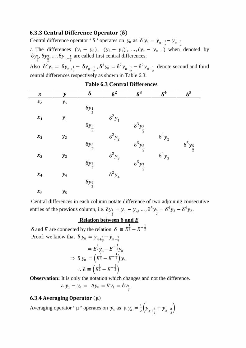
6.3.3 Central Difference Operator 𝛅
Central difference operator ‘ δ ’ operates on 𝑦𝑛 as δ 𝑦𝑛 = 𝑦𝑛+
1
2
− 𝑦𝑛−
1
2
∴ The differences (𝑦1 − 𝑦0) , (𝑦2 − 𝑦1) , … , (𝑦𝑛 − 𝑦𝑛−1) when denoted by
δ𝑦1
2
, δ𝑦3
2
, … , δ𝑦𝑛−
1
2
are called first central differences.
Also δ2𝑦𝑛 = δ𝑦𝑛+
1
2
− δ𝑦𝑛−
1
2
, δ3𝑦𝑛 = δ2𝑦𝑛+
1
2
− δ2𝑦𝑛−
1
2
denote second and third
central differences respectively as shown in Table 6.3.
Table 6.3 Central Differences
𝒙 𝒚 𝛅 𝛅𝟐 𝛅𝟑 𝛅𝟒 𝛅𝟓 𝒙𝒐 𝑦𝑜
δ𝑦12
𝒙𝟏 𝑦1 δ2𝑦1
δ𝑦32 δ3𝑦3
2
𝒙𝟐 y2 δ2𝑦2 δ4𝑦
2
δ𝑦52 δ3𝑦5
2
δ5𝑦52
𝒙𝟑 𝑦3 δ2𝑦3 δ4𝑦
3
δ𝑦72 δ3𝑦7
2
𝒙𝟒 𝑦4 δ2𝑦4
δ𝑦92
𝒙𝟓 𝑦5
Central differences in each column notate difference of two adjoining consecutive
entries of the previous column, i.e. δ𝑦1
2
= 𝑦1− 𝑦
𝑜, … , δ5𝑦5
2
= δ4𝑦3 − δ4𝑦2.
Relation between 𝛅 and 𝑬
δ and 𝐸 are connected by the relation δ ≡ 𝐸1
2 − 𝐸− 1
2
Proof: we know that δ 𝑦𝑛 = 𝑦𝑛+
1
2
− 𝑦𝑛−
1
2
= 𝐸1
2𝑦𝑛− 𝐸− 1
2𝑦𝑛
⇒ δ 𝑦𝑛 = 𝐸1
2 − 𝐸− 1
2 𝑦𝑛
∴ δ ≡ 𝐸1
2 − 𝐸− 1
2
Observation: It is only the notation which changes and not the difference.
∴ 𝑦1 − 𝑦𝑜 = ∆𝑦0 = ∇𝑦1 = δ𝑦1
2
6.3.4 Averaging Operator 𝛍
Averaging operator ‘ μ ’ operates on 𝑦𝑥 as μ 𝑦𝑥 =1
2 𝑦
𝑥+
2
+ 𝑦𝑥−
2
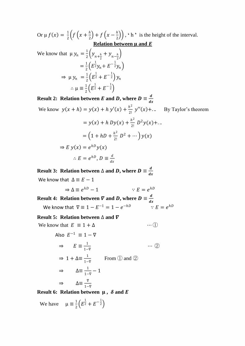
Or μ 𝑓 𝑥 = 1
2 𝑓 𝑥 +
2 + 𝑓 𝑥 −
2 , ‘ h ’ is the height of the interval.
Relation between 𝛍 and 𝑬
We know that μ 𝑦𝑛 =1
2 𝑦
𝑛+
2
+ 𝑦𝑛−
2
=1
2 𝐸
1
2𝑦𝑛+ 𝐸− 1
2𝑦𝑛
⇒ μ 𝑦𝑛 =1
2 𝐸
1
2 + 𝐸− 1
2 𝑦𝑛
∴ μ ≡1
2 𝐸
1
2 + 𝐸− 1
2
Result 2: Relation between 𝑬 and 𝑫, where 𝑫 ≡𝒅
𝒅𝒙
We know 𝑦 𝑥 + = 𝑦 𝑥 + 𝑦′ 𝑥 +2
2! 𝑦′′ 𝑥 +. .. By Taylor’s theorem
= 𝑦 𝑥 + 𝐷𝑦(𝑥) +2
2! 𝐷2𝑦(𝑥)+. ..
= 1 + 𝐷 +2
2! 𝐷2 + ⋯ 𝑦(𝑥)
⇒ 𝐸 𝑦 𝑥 = 𝑒𝐷𝑦(𝑥)
∴ 𝐸 = 𝑒𝐷, 𝐷 ≡𝑑
𝑑𝑥
Result 3: Relation between ∆ and 𝑫, where 𝑫 ≡𝒅
𝒅𝒙
We know that ∆ ≡ 𝐸 − 1
⇒ ∆ ≡ 𝑒𝐷 − 1 ∵ 𝐸 = 𝑒𝐷
Result 4: Relation between 𝜵 and 𝑫, where 𝑫 ≡𝒅
𝒅𝒙
We know that ∇ ≡ 1 − 𝐸−1 = 1 − 𝑒−𝐷 ∵ 𝐸 = 𝑒𝐷
Result 5: Relation between ∆ and 𝜵
We know that 𝐸 ≡ 1 + ∆ ⋯①
Also 𝐸−1 ≡ 1 − ∇
⇒ 𝐸 ≡1
1−∇ ⋯ ②
⇒ 1 + ∆≡1
1−∇ From ① and ②
⇒ ∆≡1
1−∇− 1
⇒ ∆≡∇
1−∇
Result 6: Relation between 𝛍 , 𝜹 and 𝑬
We have μ ≡1
2 𝐸
1
2 + 𝐸− 1
2
Also δ ≡ 𝐸1
2 − 𝐸− 1
2
⇒ μδ ≡1
2 𝐸
1
2 + 𝐸− 1
2 𝐸1
2 − 𝐸− 1
2
⇒ μδ ≡1
2 𝐸 − 𝐸− 1
Result 7: Relation between 𝛍 , 𝜹 , ∆ and ∇
We have μδ ≡1
2 𝐸 − 𝐸− 1 =
1
2 1 + ∆) − (1 − ∇
⇒ μδ ≡1
2 ∆ + ∇
Result 8: ∆𝑛𝑦𝑟 = ∇𝑛𝑦𝑛+𝑟
We have ∆𝑛𝑦𝑟 = (𝐸 − 1)𝑛𝑦𝑟 ∵ ∆= 𝐸 − 1
= 𝑦𝑛+𝑟 − 𝑛𝐶1𝑦𝑛+𝑟−1 + 𝑛𝐶2𝑦𝑛+𝑟−2 −⋯+ −1 𝑟𝑦𝑟
= 𝐸𝑛 − 𝑛𝐶1𝐸𝑛−1 + 𝑛𝐶2𝐸
𝑛−2 −⋯+ −1 𝑛 𝑦𝑟
= 𝐸𝑛𝑦𝑟 − 𝑛𝐶1𝐸𝑛−1𝑦𝑟 + 𝑛𝐶2𝐸
𝑛−2𝑦𝑟 −⋯+ −1 𝑛𝑦𝑟
= 𝑦𝑛+𝑟 − 𝑛𝐶1𝑦𝑛+𝑟−1 + 𝑛𝐶2𝑦𝑛+𝑟−2 −⋯+ −1 𝑛𝑦𝑟
Also ∇𝑛𝑦𝑛+𝑟 = (1 − E−1)𝑛𝑦𝑛+𝑟 ∵ ∇ ≡ 1 − 𝐸−1
= 1 − 𝑛𝐶1𝐸−1 + 𝑛𝐶2𝐸
−2 −⋯+ −1 𝑛𝐸−𝑛 𝑦𝑛+𝑟
= 𝑦𝑛+𝑟 − 𝑛𝐶1𝑦𝑛+𝑟−1 + 𝑛𝐶2𝑦𝑛+𝑟−2 −⋯+ −1 𝑛𝑦𝑟
∴ ∆𝑛𝑦𝑟 = ∇𝑛𝑦𝑛+𝑟
Example 1 Evaluate the following:
i. ∆𝑒𝑥 ii. ∆2𝑒𝑥 iii. ∆ 𝑡𝑎𝑛−1𝑥 iv. ∆ 𝑥+1
𝑥2−3𝑥+2 v. ∆𝑓𝑘
2 = 𝑓𝑘 + 𝑓𝑘+1 ∆𝑓𝑘
Solution: i. ∆𝑒𝑥 = 𝑒𝑥+ − 𝑒𝑥 = 𝑒𝑥(𝑒 − 1)
∆𝑒𝑥 = 𝑒𝑥(𝑒 − 1) , if = 1
ii. ∆2𝑒𝑥 = ∆(∆𝑒𝑥)
= ∆ 𝑒𝑥 𝑒 − 1
= 𝑒 − 1 ∆𝑒𝑥
= 𝑒 − 1 𝑒𝑥+ − 𝑒𝑥
= 𝑒 − 1 𝑒𝑥(𝑒 − 1)
= 𝑒𝑥 (𝑒 − 1)2
iii. ∆𝑡𝑎𝑛−1𝑥 = 𝑡𝑎𝑛−1 𝑥 + − 𝑡𝑎𝑛−1𝑥
= 𝑡𝑎𝑛−1 𝑥+−𝑥
1+(𝑥+)𝑥
= 𝑡𝑎𝑛−1
1+(𝑥+)𝑥
iv. ∆ 𝑥+1
𝑥2−3𝑥+2 = ∆
𝑥+1
𝑥−1 (𝑥−2)

= ∆ −2
𝑥−1+
3
𝑥−2 = ∆
−2
𝑥−1 + ∆
3
𝑥−2
= −2 1
𝑥+1−1−
1
𝑥−1 + 3
1
𝑥+1−2−
1
𝑥−2
= −2 1
𝑥−
1
𝑥−1 + 3
1
𝑥−1−
1
𝑥−2
= −(𝑥+4)
𝑥 𝑥−1 (𝑥−2)
v. ∆𝑓𝑘2 = 𝑓𝑘+1
2 − 𝑓𝑘2 = 𝑓𝑘+1 + 𝑓𝑘 𝑓𝑘+1 − 𝑓𝑘 = 𝑓𝑘 + 𝑓𝑘+1 ∆𝑓𝑘
Example 2 Evaluate the following:
i. ∆𝑒𝑥 log 2𝑥 ii. ∆ 𝑥2
cos 2𝑥
Solution: i. Let 𝑓 𝑥 = 𝑒𝑥 and 𝑔 𝑥 = log 2𝑥
We have ∆ 𝑓 𝑥 𝑔 𝑥 = 𝑓 𝑥 + ∆ 𝑔 𝑥 + 𝑔 𝑥 ∆𝑓 𝑥
∴ ∆𝑒𝑥 log 2𝑥 = 𝑒𝑥+∆ log 2𝑥 + log 2𝑥 ∆𝑒𝑥
= 𝑒𝑥+ log 2 𝑥 + − log 2𝑥 + log 2𝑥 𝑒𝑥+ − 𝑒𝑥
= 𝑒𝑥𝑒 log 1 +
𝑥 + 𝑒𝑥 log 2𝑥 𝑒 − 1
= 𝑒𝑥 𝑒 log 1 +
𝑥 + log 2𝑥 𝑒 − 1
ii. Let 𝑓 𝑥 = 𝑥2 and 𝑔 𝑥 = cos 2𝑥
We have ∆ 𝑓 𝑥
𝑔 𝑥 =
𝑔 𝑥 ∆𝑓 𝑥 −𝑓(𝑥)∆𝑔 𝑥
𝑔 𝑥+ 𝑔 𝑥
=cos 2𝑥 𝑥+ 2−𝑥2 −𝑥2 cos 2 𝑥+ −cos 2𝑥
cos 2 𝑥+ cos 2𝑥
= 2+2𝑥 cos 2𝑥+2𝑥2 sin 2𝑥+ sin
cos 2 𝑥+ cos 2𝑥
Example 3 Evaluate ∆4 1 − 2𝑥 1 − 3𝑥 1 − 4𝑥 1 − 𝑥 ,where interval of differencing is one.
Solution: ∆4 1 − 2𝑥 1 − 3𝑥 1 − 4𝑥 1 − 𝑥
= ∆4 24𝑥4 + ⋯+ 1 = 24.4!. 14 = 576
∵ ∆𝑛𝑓 𝑥 = 𝑎0𝑛! 𝑛 and ∆4𝑥𝑛 = 0 when 𝑛 < 4
Example 4 Prove that ∆3𝑦3 = ∇3𝑦6
Solution: ∆3𝑦3 = (𝐸 − 1)3𝑦3 ∵ ∆= 𝐸 − 1
= 𝐸3 − 1 − 3𝐸2 + 3𝐸 𝑦3
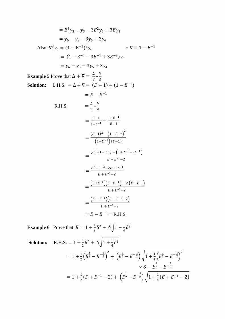
= 𝐸3𝑦3 − 𝑦3 − 3𝐸2𝑦3 + 3𝐸𝑦3
= 𝑦6 − 𝑦3 − 3𝑦5 + 3𝑦4
Also ∇3𝑦6 = (1 − E−1)3𝑦6 ∵ ∇ ≡ 1 − 𝐸−1
= 1 − E−3 − 3𝐸−1 + 3𝐸−2 𝑦6
= 𝑦6 − 𝑦3 − 3𝑦5 + 3𝑦4
Example 5 Prove that ∆ + ∇ = ∆
∇–∇
∆
Solution: L.H.S. = ∆ + ∇ = 𝐸 − 1 + 1 − 𝐸−1
= 𝐸 − 𝐸−1
R.H.S. =∆
∇–∇
∆
=𝐸−1
1−𝐸–1−
1−𝐸 –1
𝐸−1
= 𝐸−1 2 − 1− 𝐸 –1
2
1−𝐸 –1 𝐸−1
= 𝐸2+1− 2𝐸 − 1+ 𝐸–2−2𝐸–1
𝐸 + 𝐸–1−2
=𝐸2−𝐸−2−2𝐸+2𝐸–1
𝐸 + 𝐸–1−2
= 𝐸+𝐸–1 𝐸−𝐸 –1 − 2 𝐸− 𝐸–1
𝐸 + 𝐸–1−2
= 𝐸 − 𝐸–1 𝐸 + 𝐸 –1−2
𝐸 + 𝐸–1−2
= 𝐸 − 𝐸−1 = R.H.S.
Example 6 Prove that 𝐸 = 1 +1
2δ2 + δ 1 +
1
4δ2
Solution: R.H.S. = 1 +1
2δ2 + δ 1 +
1
4δ2
= 1 +1
2 𝐸
1
2 − 𝐸− 1
2 2
+ 𝐸1
2 − 𝐸− 1
2 1 +1
4 𝐸
1
2 − 𝐸− 1
2 2
∵ δ ≡ 𝐸1
2 − 𝐸− 1
2
= 1 +1
2 𝐸 + 𝐸−1 − 2 + 𝐸
1
2 − 𝐸− 1
2 1 +1
4 𝐸 + 𝐸−1 − 2

= 1 +1
2 𝐸 + 𝐸−1 − 2 + 𝐸
1
2 − 𝐸− 1
2 1
4 𝐸 + 𝐸−1 + 2
= 1 +1
2 𝐸 + 𝐸−1 − 2 + 𝐸
1
2 − 𝐸− 1
2 1
4 𝐸
1
2 + 𝐸− 1
2 2
= 1 +1
2 𝐸 + 𝐸−1 − 2 +
1
2 𝐸
1
2 − 𝐸− 1
2 𝐸1
2 + 𝐸− 1
2
=1
2 𝐸 + 𝐸−1 +
1
2 𝐸 − 𝐸−1 = 𝐸 = L.H.S.
Example 7 Prove that ∇ = −1
2δ2 + δ 1 +
1
4δ2
Solution: R.H.S. = −1
2δ2 + δ 1 +
1
4δ2
= −1
2 𝐸
1
2 − 𝐸− 1
2 2
+ 𝐸1
2 − 𝐸− 1
2 1 +1
4 𝐸
1
2 − 𝐸− 1
2 2
∵ δ ≡ 𝐸1
2 − 𝐸− 1
2
= −1
2 𝐸 + 𝐸−1 − 2 + 𝐸
1
2 − 𝐸− 1
2 1 +1
4 𝐸 + 𝐸−1 − 2
= −1
2 𝐸 + 𝐸−1 − 2 + 𝐸
1
2 − 𝐸− 1
2 1
4 𝐸 + 𝐸−1 + 2
= −1
2 𝐸 + 𝐸−1 − 2 + 𝐸
1
2 − 𝐸− 1
2 1
4 𝐸
1
2 + 𝐸− 1
2 2
= −1
2 𝐸 + 𝐸−1 − 2 +
1
2 𝐸
1
2 − 𝐸− 1
2 𝐸1
2 + 𝐸− 1
2
= −1
2 𝐸 + 𝐸−1 − 2 +
1
2 𝐸 − 𝐸−1 = 1 − 𝐸−1 = ∇= L.H.S.
Example 8 Prove that (i) ∆ − ∇ = δ2 (ii) μ = 1 +1
4δ2 = 1 +
∆
2 1 + ∆ −
1
2
Solution: (i) δ2 = 𝐸1
2 − 𝐸− 1
2 2
= 𝐸 + 𝐸−1 − 2 ∵ δ ≡ 𝐸1
2 − 𝐸− 1
2
= 𝐸 − 1 − 1 − 𝐸−1 = ∆ − ∇
∵ 𝐸 − 1 ≡ ∆ and 1 − 𝐸−1 = ∆
(ii) 1 +1
4δ2 = 1 +
1
4 𝐸
1
2 − 𝐸− 1
2 2
∵ δ ≡ 𝐸1
2 − 𝐸− 1
2
= 1 +1
4 𝐸 + 𝐸−1 − 2
= 1
4 𝐸 + 𝐸−1 + 2
= 1
4 𝐸
1
2 + 𝐸− 1
2 2

=1
2 𝐸
1
2 + 𝐸− 1
2 = μ ∵ μ ≡1
2 𝐸
1
2 + 𝐸− 1
2
Also 1 +∆
2 1 + ∆ −
1
2 = 1 +𝐸−1
2 1 + 𝐸 − 1 −
1
2
∵ ∆ ≡ 𝐸 − 1
= 𝐸+1
2 𝐸−
1
2
=1
2 𝐸−
1
2 + 𝐸1
2 = μ
Example 9 Prove that (i) ∆ ≡ 𝐸∇ ≡ ∇E = δ𝐸 12 (ii) Er = μ +
𝛿
2
2𝑟
Solution: (i) 𝐸∇ = E 1 − 𝐸− 1 = 𝐸 − 1 = ∆ ∵ ∇ ≡ 1 − 𝐸−1
∇E = 1 − 𝐸− 1 𝐸 = 𝐸 − 1 = ∆
δ𝐸 12 = 𝐸
1
2 − 𝐸− 1
2 𝐸 12 = 𝐸 − 1 = ∆ ∵ δ ≡ 𝐸
1
2 − 𝐸− 1
2
(ii) R.H.S. = μ +𝛿
2
2𝑟
= 1
2 𝐸
1
2 + 𝐸− 1
2 +1
2 𝐸
1
2 − 𝐸− 1
2
2𝑟
∵ μ ≡1
2 𝐸
1
2 + 𝐸− 1
2 and δ ≡ 𝐸1
2 − 𝐸− 1
2
= 1
2 2𝐸
1
2
2𝑟
= 𝐸1
2 2𝑟
= Er = L.H.S
Example 10 Prove that (i) 𝐷 ≡ 1
𝑙𝑜𝑔 𝐸 (iii) 𝐷 ≡ 𝑙𝑜𝑔 1 + ∆ ≡ −log(1 − ∇)
(iii) ∇2 ≡ 2𝐷2 − 3𝐷3 +7
124𝐷4 + ⋯
Solution: (i) We know that 𝐸 ≡ 𝑒𝐷
⇒ 𝑙𝑜𝑔𝐸 ≡ 𝑙𝑜𝑔 𝑒𝐷
⇒ 𝑙𝑜𝑔𝐸 ≡ 𝑑 𝑙𝑜𝑔 𝑒
⇒ 𝐷 ≡ 1
𝑙𝑜𝑔 𝐸 ∵ 𝑙𝑜𝑔 𝑒 = 1
(ii) 𝐷 ≡ 𝑙𝑜𝑔𝐸 From relation (i)
≡ log(1 + ∆) ∵ 𝐸 ≡ 1 + ∆
Also 𝐷 ≡ 𝑙𝑜𝑔𝐸 ≡ − log𝐸−1
≡ −log(1 − ∇) ∵ ∇ ≡ 1 − 𝐸−1
(iii) We know that ∇ ≡ 1 − 𝐸−1
⇒ ∇ ≡ 1 −1
𝐸

≡ 1 − 𝑒−𝐷 ∵ 𝐸 = 𝑒𝐷
⇒ ∇≡ 1 − 1 − 𝑑 +2𝐷2
2!−
3𝐷3
3!+ ⋯
⇒ ∇≡ 𝑑 −2𝐷2
2! +
3𝐷3
3!+ ⋯
∴ ∇2 ≡ 𝑑 −2𝐷2
2! +
3𝐷3
3!+ ⋯
2
⇒ ∇2 ≡ 2𝐷2 + 2𝐷2
2!
2
+ ⋯− 2 𝑑 2𝐷2
2! + 2 𝑑
3𝐷3
3! −⋯
⇒ ∇2 ≡ 2𝐷2 − 3𝐷3 + 4𝐷4
4+
4𝐷4
3 −⋯
⇒ ∇2 ≡ 2𝐷2 − 3𝐷3 +7
124𝐷4 −⋯
Remark: In order to prove any relation, we can express the operators (∆ ,∇,𝛿) in
terms of fundamental operator 𝐸.
Example 11 Form the forward difference table for the function
𝑓 𝑥 = 𝑥3 − 2𝑥2 − 3𝑥 − 1 for 𝑥 = 0, 1, 2, 3, 4.
Hence or otherwise find ∆3𝑓 𝑥 , also show that ∆4𝑓 𝑥 = 0
Solution: 𝑓 0 = −1, 𝑓 1 = −5, 𝑓 2 = −7, 𝑓 3 = −1, 𝑓 4 = 19
Constructing the forward difference table:
𝒙 𝒇(𝒙) ∆ ∆𝟐 ∆𝟑 ∆𝟒 𝟎 −1 −4
1 −5 2 −2 6 𝟐 −7 8 0 6 6 𝟑 −1 14 20 𝟒 19
From the table, we see that ∆3𝑓 𝑥 = 6 and ∆4𝑓 𝑥 = 0
Note: Using the formula ∆𝑛𝑓 𝑥 = 𝑎0𝑛! 𝑛 , ∆3𝑓 𝑥 = 1.3!. 1𝑛 = 6
Also ∆𝑛+1𝑓 𝑥 = 0 for a polynomial of degree 𝑛, ∴ ∆4𝑓 𝑥 = 0
Example 12 If for a polynomial, five observations are recorded as: 𝑦0 = −8,
𝑦1 = −6, 𝑦2 = 22, 𝑦3 = 148, 𝑦4 = 492, find 𝑦5.
Solution: 𝑦5 = 𝐸5𝑦0 = (1 + ∆)5𝑦0 ∵ 𝐸 ≡ 1 + ∆
= 𝑦0 + 5𝐶1∆𝑦0 + 5𝐶2∆2𝑦0 + 5𝐶3∆
3𝑦0 + 5𝐶4∆4𝑦0 + ∆5𝑦0 …①

Constructing the forward difference table:
𝒙 𝒚 ∆ ∆𝟐 ∆𝟑 ∆𝟒 𝒙𝟎 −8
2 𝒙𝟏 −6 26
28 72 𝒙𝟐 22 98 48
126 120 𝒙𝟑 148 218
344 𝒙𝟒 492
From table ∆𝑦0 = 2, ∆2𝑦0 = 26 , ∆3𝑦0 = 72 , ∆3𝑦0 = 48 … ②
⇒ 𝑦5
= −8 + 5 2 + 10 26 + 10 72 + 5 48 = 1222 using ② in ①
6.4 Missing values of Data Missing data or missing values occur when an observation is missing for a
particular variable in a data sample. Concept of finite differences can help to locate
the requisite value using known concepts of curve fitting.
To determine the equation of a line (equation of degree one), we need at least two
given points. Similarly to trace a parabola (equation of degree two), at least three
points are imperative. Thus we essentially require 𝑛 + 1 known observations to
determine a polynomial of 𝑛𝑡 degree.
To find missing values of data using finite differences, we presume the degree of
the polynomial by the number of known observations and use the result
∆𝑛+1𝑓 𝑥 = 0 for a polynomial of degree 𝑛.
Example 13 Use the concept of missing data to find 𝑦5 if 𝑦0 = −8, 𝑦1 = −6,
𝑦2 = 22, 𝑦3 = 148, 𝑦4 = 492
Solution: Constructing the forward difference table taking 𝑦5 as missing value
𝒙 𝒚 ∆ ∆𝟐 ∆𝟑 ∆𝟒 ∆𝟓 𝒙𝒐 −8
2 𝒙𝟏 −6 26
28 72 𝒙𝟐 22 98 48
126 120 𝑦5 − 1222 𝒙𝟑 148 218 𝑦5 − 1174
344 𝑦5 − 1054 𝒙𝟒 492 𝑦5 − 836
𝑦5 − 492 𝒙𝟓 𝑦5

Since 5 observations are known, let us assume that the polynomial represented by
given data is of 4𝑡 degree. ∴ ∆5𝑦 = 0 ⇒ 𝑦5− 1222 = 0 or 𝑦5 = 1222
Example 14 Find the missing values in the following table
𝒙 𝟎 𝟓 𝟏𝟎 𝟏𝟓 𝟐𝟎 𝟐𝟓
𝒇(𝒙) 6 ? 13 17 22 ?
Solution: Since there are 4 known values of 𝑓 𝑥 in the given data, let us assume
the polynomial represented by the given data to be of 3𝑟𝑑degree.
Constructing the forward difference table taking missing values as 𝑎 and 𝑏.
𝒙 𝒚 ∆ ∆𝟐 ∆𝟑 ∆𝟒 𝟎 6
𝑎 − 6 𝟓 𝑎 19 − 2𝑎
13 − 𝑎 3𝑎 − 28 𝟏𝟎 13 𝑎 − 9 38 − 4𝑎
4 10 − 𝑎 15 17 1 𝑎 + 𝑏 − 38
5 𝑏 − 28 2𝟎 22 𝑏 − 27
𝑏 − 22
25 𝑏
Since the polynomial represented by the given data is considered to be of
3𝑟𝑑degree, 4𝑡ℎand higher order differences are zero i.e. ∆4𝑦 = 0
∴ 38 − 4𝑎 = 0 and 𝑎 + 𝑏 − 38 = 0 Solving these two equations, we get 𝑎 = 9.5 𝑏 = 28.5
6.5 Finding Differences Using Factorial Notation We can conveniently find the forward differences of a polynomial using factorial
notation.
6.5.1 Factorial Notation of a Polynomial
A product of the form 𝑥 𝑥 − 1 𝑥 − 2 … 𝑥 − 𝑟 + 1 is called a factorial
polynomial and is denoted by 𝑥 𝑟
∴ 𝑥 = 𝑥
𝑥 2 = 𝑥(𝑥 − 1)
𝑥 3 = 𝑥 𝑥 − 1 (𝑥 − 2)
⋮
𝑥 𝑛 = 𝑥 𝑥 − 1 𝑥 − 2 … 𝑥 − 𝑛 + 1
In case, the interval of differencing is , then
𝑥 𝑛 = 𝑥 𝑥 − 𝑥 − … 𝑥 − 𝑛– 1

The results of differencing 𝑥 𝑟 are analogous to that differentiating 𝑥𝑟
∴ ∆ 𝑥 𝑛 = 𝑛 𝑥 𝑛−1
∆2 𝑥 𝑛 = 𝑛(𝑛 − 1) 𝑥 𝑛−2
∆3 𝑥 𝑛 = 𝑛 𝑛 − 1 (𝑛 − 2) 𝑥 𝑛−3
⋮
∆𝑛 𝑥 𝑛 = 𝑛 𝑛 − 1 𝑛 − 2 … 3.2.1 = 𝑛!
∆𝑛+1 𝑥 𝑛 = 0
Also 1
∆ 𝑥 =
𝑥 2
2 ,
1
∆ 𝑥 2 =
𝑥 3
3 and so on
1
∆2 𝑥 =
1
∆ 𝑥 2
2 =
𝑥 3
6
⋮
Remark:
i. Every polynomial of degree 𝑛 can be expressed as a factorial
polynomial of the same degree and vice-versa.
ii. The coefficient of highest power of 𝑥 and also the constant term
remains unchanged while transforming a polynomial to factorial
notation.
Example15 Express the polynomial 2𝑥2 + 3𝑥 + 1 in factorial notation.
Solution: 2𝑥2 − 3𝑥 + 1 = 2𝑥2 − 2𝑥 + 5𝑥 + 1
= 2𝑥 𝑥 − 1 + 5𝑥 + 1
= 2 𝑥 2 + 5 𝑥 + 1
Example16 Express the polynomial 2𝑥3 − 𝑥2 + 3𝑥 − 4 in factorial notation.
Solution: 2𝑥3 − 𝑥2 + 3𝑥 − 4 = 2 𝑥 3 + 𝐴 𝑥 2 + 𝐵 𝑥 − 4
Using remarks i and ii
= 2𝑥 𝑥 − 1 𝑥 − 2 + 𝐴𝑥 𝑥 − 1 + 𝐵𝑥 − 4
= 2𝑥3 + 𝐴 − 6 𝑥2 + −𝐴 + 𝐵 + 4 𝑥 − 4
Comparing the coefficients on both sides
A − 6 = −1, −𝐴 + B + 4 = 3
⇒ A = 5, B = 4
∴ 2𝑥3 − 𝑥2 + 3𝑥 − 4 = 2 𝑥 3 + 5 𝑥 2 + 4 𝑥 − 4
We can also find factorial polynomial using synthetic division as shown:
Coefficients 𝐴 and 𝐵 can be found as remainders under 𝑥2 and 𝑥 columns
𝑥3 𝑥2 𝑥
1 2 –1 3 –4
– 2 1
2 2 1 4 = 𝐵
– 4
2 5 = A

Example 17 Find ∆3𝑓 𝑥 for the polynomial 𝑓 𝑥 = 𝑥3 − 2𝑥2 − 3𝑥 − 1
Also show that ∆4𝑓 𝑥 = 0
Solution: Finding factorial polynomial of 𝑓 𝑥 as shown:
Let 𝑥3 − 2𝑥2 − 3𝑥 − 1 = 𝑥 3 + 𝐴 𝑥 2 + 𝐵 𝑥 − 1
Coefficients 𝐴 and 𝐵 can be found as remainders under 𝑥2 and 𝑥 columns
𝑥3 𝑥2 𝑥
1 1 –2 –3 –1
– 1 –1
2 1 –1 – 4 = 𝐵
– 2
1 1 = A
∴ 𝑓 𝑥 = 𝑥3 − 2𝑥2 − 3𝑥 − 1 = 𝑥 3 + 𝑥 2 − 4 𝑥 − 1
∆3𝑓 𝑥 = ∆3 𝑥 3 + 𝑥 2 − 4 𝑥 − 1
= 3! + 0 = 6 ∵ ∆𝑛 𝑥 𝑛 = 𝑛! and ∆𝑛+1 𝑥 𝑛 = 0
Also ∆4𝑓 𝑥 = ∆4 𝑥 3 + 𝑥 2 − 4 𝑥 − 1 = 0
Note: Results obtained are same as in Example 11, where we have used
forward difference table to compute the differences.
Example 18: Obtain the function whose first difference is 8𝑥3 − 3𝑥2 + 3𝑥 − 1
Solution: Let 𝑓 𝑥 be the function whose first difference is 8𝑥3 − 3𝑥2 + 3𝑥 − 1
⇒ ∆𝑓 𝑥 = 8𝑥3 − 3𝑥2 + 3𝑥 − 1
Let 8𝑥3 − 3𝑥2 + 3𝑥 − 1 = 8 𝑥 3 + 𝐴 𝑥 2 + 𝐵 𝑥 − 1
Coefficients 𝐴 and 𝐵 can be found as remainders under 𝑥2 and 𝑥 columns
𝑥3 𝑥2 𝑥
1 8 –3 3 –1
– 8 5
2 8 5 8 = 𝐵
– 16
8 21 = A
∴ ∆𝑓 𝑥 = 8𝑥3 − 3𝑥2 + 3𝑥 − 1 = 8 𝑥 3 + 21 𝑥 2 + 8 𝑥 − 1
𝑓 𝑥 = 1
∆ 8 𝑥 3 + 21 𝑥 2 + 8 𝑥 − 1
=8 𝑥 4
4+
21 𝑥 3
3+
8 𝑥 2
2− 𝑥 ∵
1
∆ 𝑥 =
𝑥 2
2 ,
1
∆ 𝑥 2 =
𝑥 3
3, …
= 2 𝑥 4 + 7 𝑥 3 + 4 𝑥 2 − [𝑥] = 2𝑥 𝑥 − 1 𝑥 − 2 𝑥 − 3 + 7𝑥 𝑥 − 1 𝑥 − 2 + 4𝑥 𝑥 − 1 − 𝑥
= 𝑥 2 𝑥 − 1 𝑥 − 2 𝑥 − 3 + 7 𝑥 − 1 𝑥 − 2 + 4 𝑥 − 1 − 1 = 𝑥 2𝑥3 − 5𝑥2 + 5𝑥 − 3 = 2𝑥4 − 5𝑥3 + 5𝑥2 − 3𝑥

⇒ 𝑓 𝑥 = 2𝑥4 − 5𝑥3 + 5𝑥2 − 3𝑥
6.6 Series Summation Using Finite Differences The method of finite differences may be used to find sum of a given series by
applying the following algorithm:
1. Let the series be represented by 𝑢0, 𝑢1 , 𝑢2 , 𝑢3, …
2. Use the relation 𝑢𝑟 = 𝐸𝑟𝑢0 to introduce the operator 𝐸 in the series.
3. Replace 𝐸 by ∆ by substituting 𝐸 ≡ 1 + ∆ and find the sum the series by
any of the applicable methods like sum of a G.P., exponential or logarithmic
series or by binomial expansion and operate term by term on 𝑢0 to find the
required sum.
Example 19 Prove the following using finite differences:
i. 𝑢0 + 𝑢1𝑥
1!+ 𝑢2
𝑥2
2!+ ⋯ = 𝑒𝑥 𝑢0 + 𝑥
∆ 𝑢0
1!+ 𝑥2 ∆2 𝑢0
2!+ ⋯
ii. 𝑢0 − 𝑢1 + 𝑢2 − 𝑢3 + ⋯ = 1
2 𝑢0 −
1
4∆ 𝑢0 +
1
8∆2 𝑢0 −⋯
Solution: i. 𝑢0 + 𝑢1𝑥
1!+ 𝑢2
𝑥2
2!+ ⋯ = 𝑢0 +
𝑥
1!𝐸𝑢0 +
𝑥2
2!𝐸2𝑢0 + ⋯
= 1 +𝑥𝐸
1!+
𝑥2𝐸2
2!𝑢0 + ⋯ 𝑢0
= 𝑒𝑥𝐸 𝑢0 = 𝑒𝑥(1+∆) 𝑢0
= 𝑒𝑥𝑒𝑥∆ 𝑢0
= 𝑒𝑥 1 +𝑥∆
1!+
𝑥2∆2
2!+ ⋯ 𝑢0
= 𝑒𝑥 𝑢0 + 𝑥∆ 𝑢0
1!+ 𝑥2 ∆2 𝑢0
2!+ ⋯
ii. 𝑢0 − 𝑢1 + 𝑢2 − 𝑢3 + ⋯ = 𝑢0 − 𝐸𝑢0 + 𝐸2𝑢0 − 𝐸3𝑢0 + ⋯
= 1 − 𝐸 + 𝐸2 − 𝐸3 + ⋯ 𝑢0
= 1 + 𝐸 −1 𝑢0
= 2 + ∆ −1 𝑢0
= 2−1 1 +∆
2 −1
𝑢0
=1
2 1 −
∆
2+
∆2
4−⋯ 𝑢0
= 1
2 𝑢0 −
1
4∆ 𝑢0 +
1
8∆2 𝑢0 −⋯
Example 20 Sum the series 12, 22, 32,…, 𝑛2 using finite differences.
Solution: Let the series 12, 22, 32,…, 𝑛2 be represented by 𝑢0, 𝑢1 , 𝑢2 ,…, 𝑢𝑛−1
∴ 𝑆 = 𝑢0 + 𝑢1 + 𝑢2 + ⋯+𝑢𝑛−1
⇒ 𝑆 = 𝑢0 + 𝐸𝑢0 + 𝐸2𝑢0 + ⋯+𝐸𝑛−1𝑢0
= 1 + 𝐸 + 𝐸2 + ⋯+ 𝐸𝑛−1 𝑢0

=1−𝐸𝑛
1−𝐸𝑢0 =
𝐸𝑛−1
𝐸−1𝑢0 ∵ 𝑆𝑛 = 𝑎
1−𝑟𝑛
1−𝑟
⇒ 𝑆 =(1+∆)𝑛−1
(1+∆)−1𝑢0
=1
∆ 1 + 𝑛∆ +
𝑛(𝑛−1)
2!∆2 +
𝑛 𝑛−1 (𝑛−2)
3!∆3 + ⋯ − 1 𝑢0
= 𝑛𝑢0 +𝑛(𝑛−1)
2!∆𝑢0 +
𝑛 𝑛−1 (𝑛−2)
3!∆2𝑢0 + ⋯
Now 𝑢0 = 12 = 1
∆𝑢0 = 𝑢1 − 𝑢0 = 22 − 12 = 3
∆2𝑢0 = ∆𝑢1 − ∆𝑢0 = 𝑢2 − 2𝑢1 + 𝑢0 = 32 − 2( 22) + 12 = 2
∆3𝑢0, ∆4𝑢0 … are all zero as given series is an expression of degree 2
∴ 𝑆 = 𝑛 + 𝑛(𝑛−1)
2! 3 +
𝑛 𝑛−1 (𝑛−2)
3! 2 + 0
= 𝑛 +3𝑛 𝑛−1
2+
𝑛 𝑛−1 𝑛−2
3
=1
6 6𝑛 + 9𝑛 𝑛 − 1 + 2𝑛 𝑛 − 1 𝑛 − 2
=1
6𝑛 6 + 9𝑛 − 9 + 2𝑛2 − 6𝑛 + 4
=1
6𝑛 2𝑛2 + 3𝑛 + 1 =
1
6𝑛 𝑛 + 1 (2𝑛 + 1)
Example 21 Prove that 𝑢0 + 𝑢1𝑥 + 𝑢2𝑥2 + ⋯ =
𝑢0
1−𝑥+
𝑥∆𝑢0
(1−𝑥)2+
𝑥2∆𝑢02
(1−𝑥)3+ ⋯
and hence evaluate 1.2 + 2.3𝑥 + 3.4𝑥2 + 4.5𝑥3 + ⋯
Solution: 𝑢0 + 𝑢1𝑥 + 𝑢2𝑥2 + ⋯ = 𝑢0 + 𝑥𝐸𝑢0 + 𝑥2𝐸
2𝑢0 + ⋯
= 1 + 𝑥𝐸 + 𝑥2𝐸2 + ⋯ 𝑢0
=1
1−𝑥𝐸𝑢0 ∵ 𝑆∞ =
𝑎
1−𝑟
=1
1−𝑥(1+∆)𝑢0 =
1
(1−𝑥)−𝑥∆𝑢0
=1
1−𝑥
1
1−𝑥∆
1−𝑥 𝑢0
=1
1−𝑥 1 −
𝑥∆
1−𝑥 −1𝑢0
=1
1−𝑥 1 +
𝑥∆
1−𝑥 +
𝑥2∆2
(1−𝑥)2+ ⋯ 𝑢0
= 𝑢0
1−𝑥+
𝑥∆𝑢0
(1−𝑥)2+
𝑥2∆𝑢02
(1−𝑥)3+ ⋯ = R.H.S.

Now to evaluate the series 1.2 + 2.3𝑥 + 3.4𝑥2 + 4.5𝑥3 + ⋯
Let 𝑢0 = 1.2 = 2, 𝑢1 = 2.3 = 6, 𝑢2 = 3.4 = 12, 𝑢3 = 4.5 = 20,…
Forming forward difference table to calculate the differences
𝒖 ∆ ∆𝟐 ∆𝟑 ∆𝟒 𝒖𝟎 = 𝟏.𝟐 = 𝟐
4 𝒖𝟏 = 𝟐.𝟑 = 𝟔 2
6 0 𝒖𝟐 = 𝟑.𝟒 = 𝟏𝟐 2 0
8 0 𝒖𝟑 = 𝟒.𝟓 = 𝟐𝟎 2
10 𝒖𝟒 = 𝟓.𝟔 = 𝟑𝟎
∴ 1.2 + 2.3𝑥 + 3.4𝑥2 + 4.5𝑥3 + ⋯ = 𝑢0
1−𝑥+
𝑥∆𝑢0
(1−𝑥)2+
𝑥2∆𝑢02
(1−𝑥)3+ ⋯
=2
1−𝑥+
4𝑥
(1−𝑥)2+
2𝑥2
(1−𝑥)3+ 0
=2
(1−𝑥)3
Exercise 6A
1. Express 𝑦4 in terms of successive forward differences.
2. Prove that ∆𝑛𝑒3𝑥+5 = 𝑒3 − 1 𝑛𝑒3𝑥+5
3. Evaluate ∆2 5𝑥+12
𝑥2+5𝑥+6
4. If 𝑢0 = 3, 𝑢1 = 12, 𝑢2 = 81, 𝑢3 = 2000, 𝑢4 = 100, calculate ∆4𝑢0.
5. Prove that μ =2+∆
2 1+∆= 1 +
1
4δ2
6. Find the missing value in the following table
𝑥 0 5 10 15 20 25
𝑦 6 10 - 17 - 31
7. Sum the series 13, 23, 33,…, 𝑛3 using finite differences.
Answers
1. 𝑦4 = 𝑦0 + 4∆𝑦0 + 6∆2𝑦0 + 4∆3𝑦0 + ∆4𝑦0
3. –3(𝑥2+9𝑥+15)
𝑥(𝑥+1)(𝑥+4)(𝑥+5)(𝑥+8)(𝑥+9)
4. −7459
6. 13.25, 22.5