6-1

Chapter 6

ELECTROSTATICPRECIPITATORS

James H. TurnerPhil A. LawlessToshiaki YamamotoDavid W. CoyResearch Triangle InstituteResearch Triangle Park, NC 27709

Gary P. GreinerJohn D. McKennaETS, Inc.Roanoke, VA 24018-4394

William M. VatavukInnovative Strategies and Economics Group, OAQPSU.S. Environmental Protection AgencyResearch Triangle Park, NC 27711

December, 1995

6-2

Contents

6.1 Process Description . . . . . . . . . . . . . . . . . . . . . . . . . . . . . . . . . . . . . . . . . . . . . . . 6-5

6.1.1 Introduction . . . . . . . . . . . . . . . . . . . . . . . . . . . . . . . . . . . . . . . . . . . . . . . 6-5

6.1.2 Types of ESPs . . . . . . . . . . . . . . . . . . . . . . . . . . . . . . . . . . . . . . . . . . . . . 6-5

6.1.2.1 Plate-Wire Precipitators . . . . . . . . . . . . . . . . . . . . . . . . . . . . . . . . 6-5

6.1.2.2 Flat Plate Precipitators . . . . . . . . . . . . . . . . . . . . . . . . . . . . . . . . . 6-7

6.1.2.3 Tubular Precipitators . . . . . . . . . . . . . . . . . . . . . . . . . . . . . . . 6-10

6.1.2.4 Wet Precipitators . . . . . . . . . . . . . . . . . . . . . . . . . . . . . . . . . . . . 6-10

6.1.2.5 Two-Stage Precipitators . . . . . . . . . . . . . . . . . . . . . . . . . . . . . . 6-10

6.1.3 Auxiliary Equipment . . . . . . . . . . . . . . . . . . . . . . . . . . . . . . . . . . . . . . . . 6-11

6.1.4 Electrostatic Precipitation Theory . . . . . . . . . . . . . . . . . . . . . . . . . . . 6-12

6.1.4.1 Electrical Operating Point . . . . . . . . . . . . . . . . . . . . . . . . . . . . . 6-13

6.1.4.2 Particle Charging . . . . . . . . . . . . . . . . . . . . . . . . . . . . . . . . . . . . 6-15

6.1.4.3 Particle Collection . . . . . . . . . . . . . . . . . . . . . . . . . . . . . . . . . . . 6-18

6.1.4.4 Sneakage and Rapping Reentrainment . . . . . . . . . . . . . . . . . . . . 6-20

6.2 ESP Design Procedure . . . . . . . . . . . . . . . . . . . . . . . . . . . . . . . . . . . . . . . . . . . . 6-21

6.2.1 Specific Collecting Area . . . . . . . . . . . . . . . . . . . . . . . . . . . . . . . . . . . . 6-21

6.2.1.1 SCA Procedure with Known Migration Velocity . . . . . . . . . . . . 6-22

6.2.1.2 Full SCA Procedure . . . . . . . . . . . . . . . . . . . . . . . . . . . . . . . . . 6-24

6.2.1.3 Specific Collecting Area for Tubular Precipitators . . . . . . . . . . 6-32

6.2.2 Flow Velocity . . . . . . . . . . . . . . . . . . . . . . . . . . . . . . . . . . . . . . . . . . . . 6-32

6.2.3 Pressure Drop Calculations . . . . . . . . . . . . . . . . . . . . . . . . . . . . . . . . . . 6-33

6-3

6.2.4 Particle Characteristics . . . . . . . . . . . . . . . . . . . . . . . . . . . . . . . . . . . . . . 6-36

6.2.5 Gas Characteristics . . . . . . . . . . . . . . . . . . . . . . . . . . . . . . . . . . . . . . . . . 6-37

6.2.6 Cleaning . . . . . . . . . . . . . . . . . . . . . . . . . . . . . . . . . . . . . . . . . . . . . . . . . 6-37

6.2.7 Construction Features . . . . . . . . . . . . . . . . . . . . . . . . . . . . . . . . . . . . . . . 6-38

6.3 Estimating Total Capital Investment . . . . . . . . . . . . . . . . . . . . . . . . . . . . . . . . . 6-39

6.3.1 Equipment Cost . . . . . . . . . . . . . . . . . . . . . . . . . . . . . . . . . . . . . . . . . . . 6-39

6.3.1.1 ESP Costs . . . . . . . . . . . . . . . . . . . . . . . . . . . . . . . . . . . . . . . . . 6-39

6.3.1.2 Retrofit Cost Factor . . . . . . . . . . . . . . . . . . . . . . . . . . . . . . . . . . 6-42

6.3.1.3 Auxiliary Equipment . . . . . . . . . . . . . . . . . . . . . . . . . . . . . . . . . 6-43

6.3.1.4 Costs for Two-Stage Precipitators . . . . . . . . . . . . . . . . . . . . . . . 6-45

6.3.2 Total Purchased Cost . . . . . . . . . . . . . . . . . . . . . . . . . . . . . . . . . . . . . . . 6-45

6.3.3 Total Capital Investment (TCI) . . . . . . . . . . . . . . . . . . . . . . . . . . . . . . . . 6-46

6.4 Estimating Total Annual Costs . . . . . . . . . . . . . . . . . . . . . . . . . . . . . . . . . . . . . . 6-46

6.4.1 Direct Annual Costs . . . . . . . . . . . . . . . . . . . . . . . . . . . . . . . . . . . . . . . . 6-46

6.4.1.1 Operating and Supervisory Labor . . . . . . . . . . . . . . . . . . . . . . . 6-46

6.4.1.2 Operating Materials . . . . . . . . . . . . . . . . . . . . . . . . . . . . . . . . . . 6-47

6.4.1.3 Maintenance . . . . . . . . . . . . . . . . . . . . . . . . . . . . . . . . . . . . . . . 6-49

6.4.1.4 Electricity . . . . . . . . . . . . . . . . . . . . . . . . . . . . . . . . . . . . . . . . . 6-49

6.4.1.5 Fuel . . . . . . . . . . . . . . . . . . . . . . . . . . . . . . . . . . . . . . . . . . . . . . 6-50

6.4.1.6 Water . . . . . . . . . . . . . . . . . . . . . . . . . . . . . . . . . . . . . . . . . . . . . 6-51

6.4.1.7 Compressed Air . . . . . . . . . . . . . . . . . . . . . . . . . . . . . . . . . . . . . 6-51

6.4.1.8 Dust Disposal . . . . . . . . . . . . . . . . . . . . . . . . . . . . . . . . . . . . . . 6-51

6.4.1.9 Wastewater Treatment . . . . . . . . . . . . . . . . . . . . . . . . . . . . . . . . 6-51

6-4

6.4.1.10 Conditioning Costs . . . . . . . . . . . . . . . . . . . . . . . . . . . . . . . . . 6-52

6.4.2 Indirect Annual Costs . . . . . . . . . . . . . . . . . . . . . . . . . . . . . . . . . . . . . . . 6-52

6.4.3 Recovery Credits . . . . . . . . . . . . . . . . . . . . . . . . . . . . . . . . . . . . . . . . . . 6-52

6.4.4 Total Annual Cost . . . . . . . . . . . . . . . . . . . . . . . . . . . . . . . . . . . . . . . . . 6-52

6.4.5 Example Problem . . . . . . . . . . . . . . . . . . . . . . . . . . . . . . . . . . . . . . . . . . 6-53

6.4.5.1 Design SCA . . . . . . . . . . . . . . . . . . . . . . . . . . . . . . . . . . . . . . . 6-53

6.4.5.2 ESP Cost . . . . . . . . . . . . . . . . . . . . . . . . . . . . . . . . . . . . . . . . . . 6-57

6.4.5.3 Costs of Auxiliaries . . . . . . . . . . . . . . . . . . . . . . . . . . . . . . . . . . 6-57

6.4.5.4 Total Capital Investment . . . . . . . . . . . . . . . . . . . . . . . . . . . . . . 6-57

6.4.5.5 Annual Costs-Pressure Drop . . . . . . . . . . . . . . . . . . . . . . . . . . . 6-58

6.4.5.8 Total Annual Cost . . . . . . . . . . . . . . . . . . . . . . . . . . . . . . . . . . . 6-61

6.5 Acknowledgments . . . . . . . . . . . . . . . . . . . . . . . . . . . . . . . . . . . . . . . . . . . . . . . . . 6-61

Appendix 6A . . . . . . . . . . . . . . . . . . . . . . . . . . . . . . . . . . . . . . . . . . . . . . . . . . . . . . . . . 6-62

References . . . . . . . . . . . . . . . . . . . . . . . . . . . . . . . . . . . . . . . . . . . . . . . . . . . . . . . . . . . 6-67

6-5

6.1 Process Description

6.1.1 Introduction

An electrostatic precipitator (ESP) is a particle control device that uses electrical forces to movethe particles out of the flowing gas stream and onto collector plates. The particles are given anelectrical charge by forcing them to pass through a corona, a region in which gaseous ions flow.The electrical field that forces the charged particles to the walls comes from electrodesmaintained at high voltage in the center of the flow lane.

Once the particles are collected on the plates, they must be removed from the plates withoutreentraining them into the gas stream. This is usually accomplished by knocking them loosefrom the plates, allowing the collected layer of particles to slide down into a hopper from whichthey are evacuated. Some precipitators remove the particles by intermittent or continuouswashing with water.

6.1.2 Types of ESPs

ESPs are configured in several ways. Some of these configurations have been developed forspecial control action, and others have evolved for economic reasons. The types that will bedescribed here are (1) the plate-wire precipitator, the most common variety; (2) the flat plateprecipitator, (3) the tubular precipitator; (4) the wet precipitator, which may have any of theprevious mechanical configurations; and (5) the two-stage precipitator.

6.1.2.1 Plate-Wire Precipitators

Plate-wire ESPs are used in a wide variety of industrial applications, including coal-fired boilers,cement kilns, solid waste incinerators, paper mill recovery boilers, petroleum refining catalyticcracking units, sinter plants, basic oxygen furnaces, open hearth furnaces, electric arc furnaces,coke oven batteries, and glass furnaces.

In a plate-wire ESP, gas flows between parallel plates of sheet metal and high-voltageelectrodes. These electrodes are long wires weighted and hanging between the plates or aresupported there by mast-like structures (rigid frames). Within each flow path, gas flow mustpass each wire in sequence as flows through the unit.

The plate-wire ESP allows many flow lanes to operate in parallel, and each lane can be quitetall. As a result, this type of precipitator is well suited for handling large volumes of gas. Theneed for rapping the plates to dislodge the collected material has caused the plat to be dividedinto sections, often three or four in series with one another, which can be rapped independent.The power supplies are often sectionalized in the same way to obtain higher operating voltages,and further electrical sectionalization may be used for increased reliability. Dust also depositson the discharge electrode wires and must be periodically removed similarly to the collectorplate.

6-6

The power supplies for the ESP convert the industrial ac voltage (220 to 480 V) to pulsatingdc voltage in the range of 20,000 to 100,000 V as needed. The supply consists of a step-uptransformer, high-voltage rectifiers, and sometimes filter capacitors. The unit may supply eitherhalf-wave or full-wave rectified dc voltage. There are auxiliary components and controls toallow the voltage to be adjusted to the highest level possible without excessive sparking and toprotect the supply and electrodes in the event a heavy arc or short-circuit occurs.

The voltage applied to the electrodes causes the air between the electrodes to break downelectrically, an action known as a "corona". The electrodes usually are given a negative polaritybecause a negative corona supports a higher voltage than a positive corona before sparkingoccurs. The ions generated in the corona follow electric field lines from the wires to thecollecting plates. Therefore, each wire establishes a charging zone through which the particlesmust pass.

Particles passing through the charging zone intercept some of the ions, which becomeattached. Small aerosol particles (<1 µm diameter) can absorb tens of ions before their totalcharge becomes large enough to repel further ions, and large particles (>10 µm diameter) canabsorb tens of thousands. The electrical forces are therefore much stronger on the large particles.

As the particles pass each successive wire, they are driven closer and closer to the collectingwalls. The turbulence in the gas, however, tends to keep them uniformly mixed with the gas.The collection process is therefore a competition between the electrical and dispersive forces.Eventually, the particles approach close enough to the walls so that the turbulence drops to lowlevels and the particles are collected.

If the collected particles could be dislodged into the hopper without losses, the ESP wouldbe extremely efficient. The rapping that dislodges the accumulated layer also projects some ofthe particles (typically 12 percent for coal fly ash) back into the gas stream. These reentrainedparticles are then processed again by later sections, but the particles reentrained in the lastsection of the ESP have no chance to be recaptured and so escape the unit.

Practical considerations of passing the high voltage into the space between the lanes andallowing for some clearance above the hoppers to support and align electrodes leave room forpart of the gas to flow around the charging zones. This is called "sneakage" and amounts to 5to 10 percent of the total flow. Antisneakage baffles usually are placed to force the sneakageflow to mix with the main gas stream for collection in later sections. But, again, the sneakageflow around the last section has no opportunity to be collected.

These losses play a significant role in the overall performance of an ESP. Another majorfactor is the resistivity of the collected material. Because the particles form a continuous layeron the ESP plates, all the ion current must pass through the layer to reach the ground-plates.This current creates an electric field in the layer, and it can become large enough to cause localelectrical breakdown. When this occurs, new ions of the wrong polarity are injected into thewire-plate gap where they reduce the charge on the particles and may cause sparking. Thisbreakdown condition is called "back corona"

6-7

Back corona is prevalent when the resistivity of the layer is high, usually above 2 x 10 ohm-11

cm. For lower resistivities, the operation of the ESP is not impaired by back coronas, butresistivities much higher than 2 x 10 ohm-cm considerably reduce the collection ability of the11

unit because the severe back corona causes difficulties in charging the particles. At resistivitiesbelow 10 ohm-cm, the particles are held on the plates so loosely that rapping and nonrapping8

reentrainment become much more severe. Care must be taken in measuring or estimatingresistivity because it is strongly affected by variables such as temperature, moisture, gascomposition, particle composition, and surface characteristics.

6.1.2.2 Flat Plate Precipitators

A significant number of smaller precipitators (100,000 to 200,000 acfm) use flat plates insteadof wires for the high-voltage electrodes. The flat plates (United McGill Corporation patents)increase the average electric field that can be used to collect the particles, and they provide anincreased surface area for the collection of particles. Corona cannot be generated on flat platesby themselves, so corona-generating electrodes are placed ahead of and sometimes behind theflat plate collecting zones. These electrodes may be sharp-pointed needles attached to the edgesof the plates or independent corona wires. Unlike place-wire or tubular ESPs, this designoperates equally well with either negative or positive polarity. The manufacturer has chosen touse positive polarity to reduce ozone generation.

A flat plate ESP operates with little or no corona current flowing through the collected dust,except directly under the corona needles or wires. This has two consequences. The first is thatthe unit is somewhat less susceptible to back corona than conventional units are because no backcorona is generated in the collected dust, and particles charged with both polarities of ions havelarge collection surfaces available. The second consequence is that the lack of current in thecollected layer causes an electrical force that tends to remove the layer from the collectingsurface; this can lead to high rapping losses.

Flat plate ESPs seem to have wide application for high-resistivity particles with small (1 to2 µm) mass median diameters (MMDs). These applications especially emphasize the strengthsof the design because the electrical dislodging forces are weaker for small particles than for largeones. Fly ash has been successfully collected with this type of ESP, but low-flow velocityappears to be critical for avoiding high rapping losses.

6-8

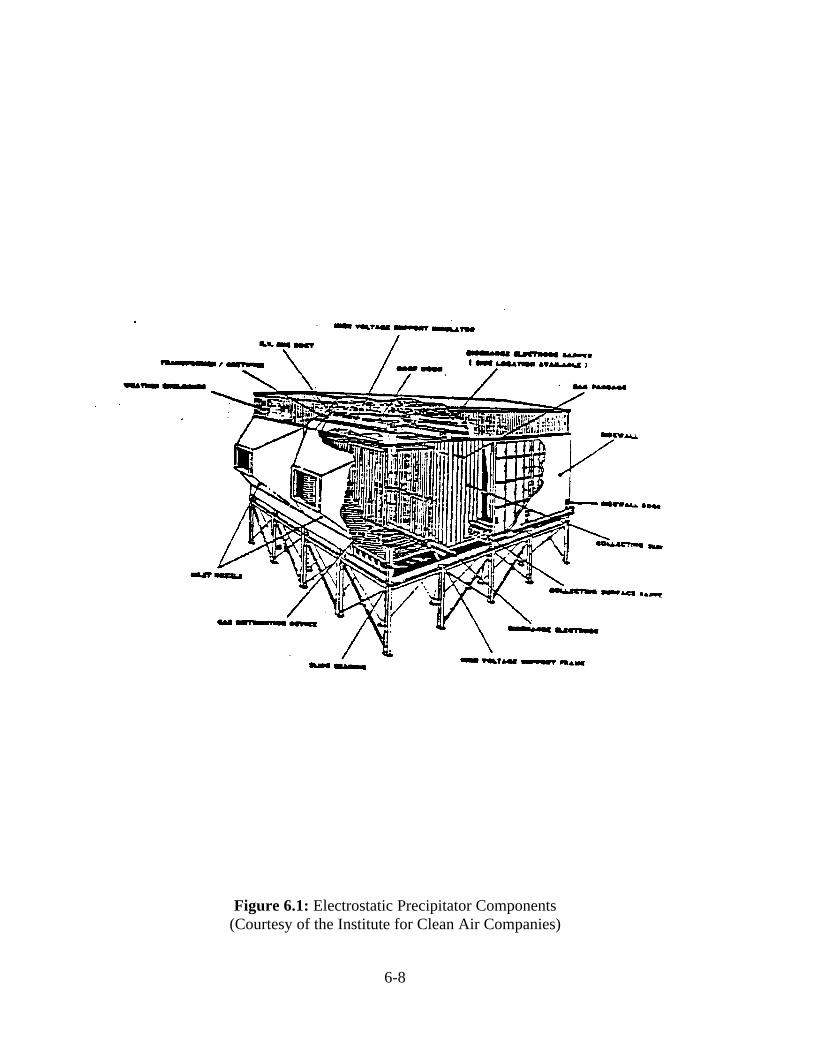
Figure 6.1: Electrostatic Precipitator Components(Courtesy of the Institute for Clean Air Companies)

6-9

Figure 6.2: Flat-plate and Plate-wire ESP Configurations(Courtesy of United McGill Corporation)

6-10

6.1.2.3 Tubular Precipitators

The original ESPs were tubular like the smokestacks they were placed on, with the high-voltageelectrode running along the axis of the tube. Tubular precipitators have typical applications insulfuric add plants, coke oven by-product gas cleaning (tar removal), and, recently, iron and steelsinter plants. Such tubular units are still used for some applications, with many tubes operatingin parallel to handle increased gas flows. The tubes may be formed as a circular, square, orhexagonal honeycomb with gas flowing upwards or downwards. The length of the tubes can beselected to fit conditions. A tubular ESP can be tightly sealed to prevent leaks of material,especially valuable or hazardous material.

A tubular ESP is essentially a one-stage unit and is unique in having all the gas pass throughthe electrode region. The high-voltage electrode operates at one voltage for the entire length ofthe tube, and the current varies along the length as the particles are removed from the system.No sneakage paths are around the collecting region, but corona nonuniformities may allow someparticles to avoid charging for a considerable fraction of the tube length.

Tubular ESPs comprise only a small portion of the ESP population and are most commonlyapplied where the particulate is either wet or sticky. These ESPs, usually cleaned with water,have reentrainment losses of a lower magnitude than do the dry particulate precipitators.

6.1.2.4 Wet Precipitators

Any of the precipitator configurations discussed above may be operated with wet walls insteadof dry. The water flow may be applied intermittently or continuously to wash the collectedparticles into a sump for disposal. The advantage of the wet wall precipitator is that it has noproblems with rapping reentrainment or with back coronas. The disadvantage is the increasedcomplexity of the wash and the fact that the collected slurry must be handled more carefully thana dry product, adding to the expense of disposal.

6.1.2.5 Two-Stage Precipitators

The previously described precipitators are all parallel in nature, i.e., the discharge and collectingelectrodes are side by side. The two-stage precipitator invented by Penney is a series device withthe discharge electrode, or ionizer, preceding the collector electrodes. For indoor applications,the unit is operated with positive polarity to limit ozone generation.

Advantages of this configuration include more time for particle charging, less propensity forback corona, and economical construction for small sizes. This type of precipitator is generallyused for gas flow volumes of 50,000 acfm and less and is applied to submicrometer sources

6-11

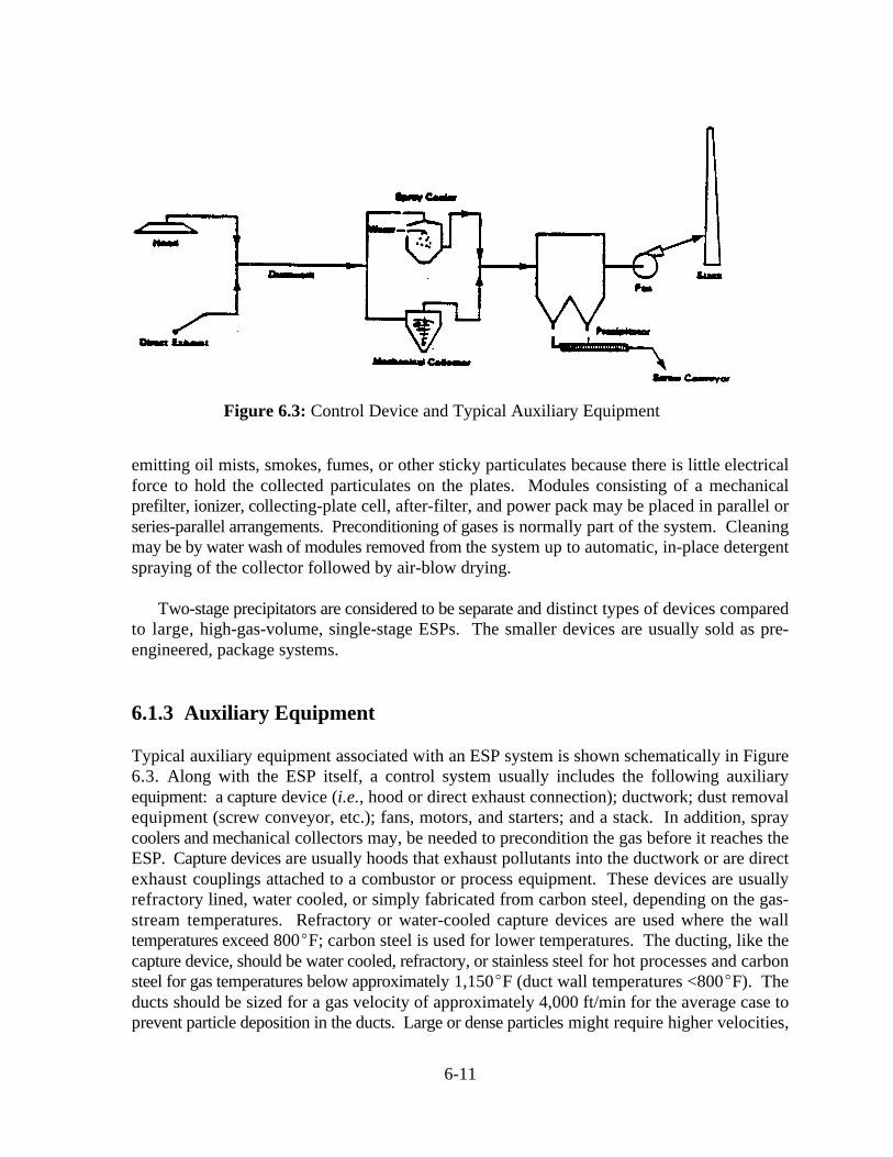
Figure 6.3: Control Device and Typical Auxiliary Equipment

emitting oil mists, smokes, fumes, or other sticky particulates because there is little electricalforce to hold the collected particulates on the plates. Modules consisting of a mechanicalprefilter, ionizer, collecting-plate cell, after-filter, and power pack may be placed in parallel orseries-parallel arrangements. Preconditioning of gases is normally part of the system. Cleaningmay be by water wash of modules removed from the system up to automatic, in-place detergentspraying of the collector followed by air-blow drying.

Two-stage precipitators are considered to be separate and distinct types of devices comparedto large, high-gas-volume, single-stage ESPs. The smaller devices are usually sold as pre-engineered, package systems.

6.1.3 Auxiliary Equipment

Typical auxiliary equipment associated with an ESP system is shown schematically in Figure6.3. Along with the ESP itself, a control system usually includes the following auxiliaryequipment: a capture device (i.e., hood or direct exhaust connection); ductwork; dust removalequipment (screw conveyor, etc.); fans, motors, and starters; and a stack. In addition, spraycoolers and mechanical collectors may, be needed to precondition the gas before it reaches theESP. Capture devices are usually hoods that exhaust pollutants into the ductwork or are directexhaust couplings attached to a combustor or process equipment. These devices are usuallyrefractory lined, water cooled, or simply fabricated from carbon steel, depending on the gas-stream temperatures. Refractory or water-cooled capture devices are used where the walltemperatures exceed 800EF; carbon steel is used for lower temperatures. The ducting, like thecapture device, should be water cooled, refractory, or stainless steel for hot processes and carbonsteel for gas temperatures below approximately 1,150EF (duct wall temperatures <800EF). Theducts should be sized for a gas velocity of approximately 4,000 ft/min for the average case toprevent particle deposition in the ducts. Large or dense particles might require higher velocities,

6-12

but rarely would lower velocities be used. Spray chambers may be required for processes wherethe addition of moisture, or decreased temperature or gas volume, will improve precipitation orprotect the ESP from warpage. For combustion processes with exhaust gas temperatures belowapproximately 700EF, cooling would not be required, and the exhaust gases can be delivereddirectly to the precipitator.

When much of the pollutant loading consists of relatively large particles, mechanicalcollectors, such as cyclones, may be used to reduce the load on the ESP, especially at high inletconcentrations. The fans provide the motive power for air movement and can be mounted beforeor after the ESP. A stack, normally used, vents the cleaned stream to the atmosphere. Screwconveyors or pneumatic systems are often used to remove captured dust from the bottom of thehoppers.

Wet ESPs require a source of wash water to be injected or sprayed near the top of thecollector plates either continuously or at timed intervals. The water flows with the collectedparticles into a sump from which the fluid is pumped. A portion of the fluid may be recycledto reduce the total amount of water required. The remainder is pumped directly to a settlingpond or passed through a dewatering stage, with subsequent disposal of the sludge.

Gas conditioning equipment to improve ESP performance by changing dust resistivity isoccasionally used as part of the original design, but more frequently it is used to upgrade existingESPs. The equipment injects an agent into the gas stream ahead of the ESP. Usually, the agentmixes with the particles and alters their resistivity to promote higher migration velocity, and thushigher collection efficiency. However, electrical properties of the gas may change, rather thandust resistivity. For instance, cooling the gas will allow more voltage to be applied beforesparking occurs. Significant conditioning agents that are used include SO , H SO , sodium3 2 4

compounds, ammonia, and water, but the major conditioning agent by usage is SO . A typical3

dose rate for any of the gaseous agents is 10 to 30 ppm by volume.

The equipment required for conditioning depends on the agent being used. A typical S03

conditioner requires a supply of molten sulfur. It is stored in a heated vessel and supplied to aburner, where it is oxidized to SO . The SO gas is passed over a catalyst for further oxidation2 2

to S0 . The S0 gas is then injected into the flue gas stream through a multi-outlet set of probes3 3

that breach a duct. In place of a sulfur burner to provide S0 , liquid S0 may be vaporized from2 2

a storage tank. Although their total annual costs are higher, the liquid SO systems have lower2

capital costs and are easier to operate than the molten sulfur based systems.

Water or ammonia injection requires a set of spray nozzles in the duct, along with pumpingand control equipment.

Sodium conditioning is often done by coating the coal on a conveyor with a powdercompound or a water solution of the desired compound. A hopper or storage tank is oftenpositioned over the conveyor for this purpose.

6.1.4 Electrostatic Precipitation Theory

Ec ' 3.126 × 106dr[1 % 0.0301(dr/rw)0.5]

6-13

(6.1)

The theory of ESP operation requires many scientific disciplines to describe it thoroughly.The ESP is basically an electrical machine. The principal actions are the charging of particlesand forcing them to the collector plates. The amount of charged particulate matter affects theelectrical operating point of the ESP. The transport of the particles is affected by the level ofturbulence in the gas. The losses mentioned earlier, sneakage and rapping reentrainment, aremajor influences on the total performance of the system. The particle properties also leave amajor effect on the operation of the unit.

The following subsections will explain the theory behind (1) electrical operating points inthe ESP, (2) particle charging, (3) particle collection, and (4) sneakage and rappingreentrainment. General references for these topics are White [1] or Lawless and Sparks [2].

6.1.4.1 Electrical Operating Point

The electrical operating point of an ESP section is the value of voltage and current at which thesection operates. As will become apparent, the best collection occurs when the highest electricfield is present, which roughly corresponds to the highest voltage on the electrodes. In this work,the term "section" represents one set of plates and electrodes in the direction of flow. This unitis commonly called a "field", and a "section" or "bus section" represents a subdivision of a"field" perpendicular to the direction of flow. In an ESP model and in sizing applications, thetwo terms "section" and "field" are used equivalently because the subdivision into bus sectionsshould have no effect on the model. This terminology has probably arisen because of thefrequent use of the word "field" to refer to the electric field.

The lowest acceptable voltage is the voltage required for the formation of a corona, theelectrical discharge that produces ions for charging particles. The (negative) corona is producedwhen an occasional free electron near the high-voltage electrode, produced by a cosmic ray,gains enough energy from the electric field to ionize the gas and produce more free electrons.The electric field for which this process is self-sustained has been determined experimentally.For round wires, the field at the surface of the wire is given by:

whereE = corona onset field at the wire surface (V/m) e

d = relative gas density, referred to 1 atm pressure and 20EC (dimensionless) r

r = radius of the wire, meters (m)w

Vc ' Ecrw lndrw

j ' µåV 2

L 3

6-14

(6.2)

(6.3)

This is the field required to produce "glow" corona, the form usually seen in the laboratoryon smooth, clean wires. The glow appears as a uniform, rapidly moving diffuse light around theelectrode. After a period of operation, the movement concentrates into small spots on the wiresurface, and the corona assumes a tuft-like appearance. The field required to produce "tuft"corona, the form found in full-scale ESPs, is 0.6 times the value of E .c

The voltage that must be applied to the wire to obtain this value of field, V , is found byc

integrating the electric field from the wire to the plate. The field follows a simple "1/r"dependence in cylindrical geometry. This leads to a logarithmic dependence of voltage onelectrode dimensions. In the plate-wire geometry, the field dependence is somewhat morecomplex, but the voltage still shows the logarithmic dependence. V is given by:c

whereV = corona onset voltage (V)c

d = outer cylinder radius for tubular ESP (m)4/ x (wire-plate separation) for plate-wire ESP (m)

No current will flow until the voltage reaches this value, but the amount of current willincrease steeply for voltages above this value. The maximum current density (amperes/squaremeter) on the plate or cylinder directly under the wire is given by:

wherej = maximum current density (A/m )2

µ = ion mobility m /Vs) (meter /volt second)2 2

= free space permittivity (8.845 x 10 F/m)(Farad/meter)-12

V = applied voltage (V)L = shortest distance from wire to collecting surface (m)

For tuft corona, the current density is zero until the corona onset voltage is reached, whenit jumps almost to this value of j within a few hundred volts, directly under a tuft.

The region near the wire is strongly influenced by the presence of ions there, and the coronaonset voltage magnitude shows strong spatial variations. Outside the corona region, it is quiteuniform.

Emax ' V/L

Es ' 6.3 × 105273T

P1.65

El ' j ñ

6-15

(6.4)

(6.5)

The electric field is strongest along the line from wire to plate and is approximated very well,except near the wire, by:

where

E = maximum field strength (V/m)max

When the electric field throughout the gap between the wire and the plate becomes strongenough, a spark will occur, and the voltage cannot be increased without severe sparkingoccurring. The field at which sparking occurs is not sharply defined, but a reasonable value isgiven by:

where

E = sparking field strength (V/m)s

T = absolute temperature (K)P = gas pressure (atm)

This field would be reached at a voltage of, for example, 35,000 V for a plate-wire spacing of11.4 cm (4.5 in.) at a temperature of 149EC (300EF). The ESP will generally operate near thisvoltage in the absence of back corona. E will be equal to or less than E .max s

Instead of sparking, back corona may occur if the electric field in the dust layer, resultingfrom the current flow in the layer, reaches a critical value of about 1 x 10 V/m. Depending on6

conditions, the back corona, may enhance sparking or may generate so much current that thevoltage cannot be raised any higher. The field in the layer is given by:

where

E = electric field in dust layer (V/m)l

= resistivity of the collected material (ohm-m)

6.1.4.2 Particle Charging

q(t) 'rkTe

ln(1 % r)

ô 'ðrv Ne 2è

kT

6-16

(6.8)

Charging of particles takes place when ions bombard the surface of a particle. Once an ion isclose to the particle, it is tightly bound because of the image charge within the particle. The"image charge" is a representation of the charge distortion that occurs when a real chargeapproaches a conducting surface. The distortion is equivalent to a charge of opposite magnitudeto the real charge, located as far below the surface as the real charge is above it. The notion ofthe fictitious charge is similar to the notion of an image in a mirror, hence the name. As moreions accumulate on a particle, the total charge tends to prevent further ionic bombardment.

There are two principal charging mechanisms: diffusion charging and field charging.Diffusion charging results from the thermal kinetic energy of the ions overcoming the repulsionof the ions already on the particle. Field charging occurs when ions follow electric field linesuntil they terminate on a particle. In general, both mechanisms are operative for all sizes ofparticles. Field charging, however, adds a larger percentage of charge on particles greater thanabout 2µm in diameter, and diffusion charging adds a greater percentage on particles smaller thanabout 0.5µm.

Diffusion charging, as derived by White [1], produces a logarithmically increasing level ofcharge on particles, given by:

where

q(t) = particle charge (C) as function of time, t, in secondsr = particle radius (m)k = Boltzmann's constant (j/K)T = absolute temperature (K)e = electron charge (1.67 x 10 C)-19

= dimensionless time given by:

wherev = mean thermal speed of the ions (m/s)N = ion number concentration near the particle (No./m ) = real time (exposure3

2 = real time (exposure time in the charging zone) (s)

Diffusion charging never reaches a limit, but it becomes very slow after about threedimensionless time units. For fixed exposure times, the charge on a particle is proportional toits radius.

q(t) ' qsè/(è % ô))

qs ' 12ð0r 2 E

r ) ' 4å/Neµ

qtot ' qd(t) % qf(t)

6-17

(6.9)

(6.10)

(6.11)

(6.12)

Field charging also exhibits a characteristic time-dependence, given by:

where

q = saturation charge, charge at infinite time (C)s

= real time (s)= another dimensionless time unit

The saturation charge is given by:

where

= free space permittivity (F/m)E = external electric field applied to the particle (V/m)

The saturation charge is proportional to the square of the radius, which explains why fieldcharging is the dominant mechanism for larger particles. The field charging time constant isgiven by:

whereµ = ion mobility

Strictly speaking, both diffusion and field charging mechanisms operate at the same time onall particles, and neither mechanism is sufficient to explain the charges measured on theparticles. It has been found empirically that a very good approximation to the measured chargeis given by the sum of the charges predicted by equations 6.7 and 6.9 independently of oneanother:

where

Fe ' qE

v(q, E, r) 'q(E, r) × E × C(r)

6ðçr

6-18

(6.13)

(6.14)

q (t) = particle charge due to both mechanisms tot

q (t) = particle charge due to diffusion charging d

q (t) = particle charge due to field chargingf

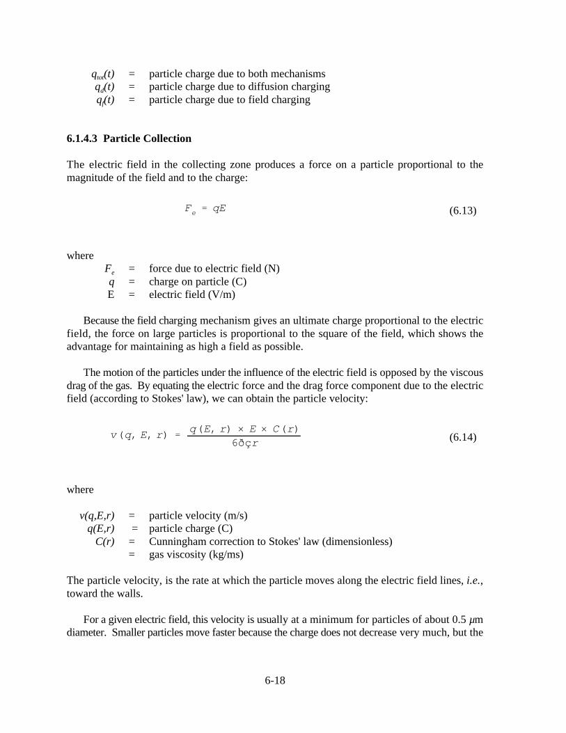
6.1.4.3 Particle Collection

The electric field in the collecting zone produces a force on a particle proportional to themagnitude of the field and to the charge:

whereF = force due to electric field (N) e

q = charge on particle (C) E = electric field (V/m)

Because the field charging mechanism gives an ultimate charge proportional to the electricfield, the force on large particles is proportional to the square of the field, which shows theadvantage for maintaining as high a field as possible.

The motion of the particles under the influence of the electric field is opposed by the viscousdrag of the gas. By equating the electric force and the drag force component due to the electricfield (according to Stokes' law), we can obtain the particle velocity:

where

v(q,E,r) = particle velocity (m/s)q(E,r) = particle charge (C)

C(r) = Cunningham correction to Stokes' law (dimensionless)= gas viscosity (kg/ms)

The particle velocity, is the rate at which the particle moves along the electric field lines, i.e.,toward the walls.

For a given electric field, this velocity is usually at a minimum for particles of about 0.5 µmdiameter. Smaller particles move faster because the charge does not decrease very much, but the

N(r) ' N0(r) × exp(&v(r)/v0)

v0 ' Q/A ' 1/SCA

p ' exp(&we × SCA)

6-19

(6.15)

(6.16)

(6.17)

Cunningham factor increases rapidly as radius decreases. Larger particles have a chargeincreasing as r and a viscous drag only increasing as r ; the velocity then increases as r.2 1

Equation 6.14 gives the particle velocity with respect to still air. In the ESP, the flow isusually very turbulent, with instantaneous gas velocities of the same magnitude as the particlesvelocities, but in random directions. The motion of particles toward the collecting plates istherefore a statistical process, with an average component imparted by the electric field and afluctuating component from the gas turbulence.

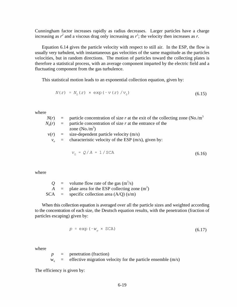
This statistical motion leads to an exponential collection equation, given by:

whereN(r) = particle concentration of size r at the exit of the collecting zone (No./m3

N (r) = particle concentration of size r at the entrance of the0

zone (No./m )3

v(r) = size-dependent particle velocity (m/s)v = characteristic velocity of the ESP (m/s), given by:o

where

Q = volume flow rate of the gas (m /s)3

A = plate area for the ESP collecting zone (m )2

SCA = specific collection area (A/Q) (s/m)

When this collection equation is averaged over all the particle sizes and weighted accordingto the concentration of each size, the Deutsch equation results, with the penetration (fraction ofparticles escaping) given by:

wherep = penetration (fraction)

w = effective migration velocity for the particle ensemble (m/s)e

The efficiency is given by:

Eff(%) ' 100(1 & p)

ps ' SN % [(1 & SN) × pc(Q))]

m/m0 ' 1 & ps ' 1 & SN & [(1 & SN) × pc(Q))]

6-20

(6.18)

(6.19)

(6.20)

and is the number most often used to describe the performance of an ESP.

6.1.4.4 Sneakage and Rapping Reentrainment

Sneakage and rapping reentrainment are best considered on the basis of the sections within anESP. Sneakage occurs when a part of the gas flow bypasses the collection zone of a section.Generally, the portion of gas that bypasses the zone is thoroughly mixed with the gas that passesthrough the zone before all the gas enters the next section. This mixing cannot always beassumed, and when sneakage paths exist around several sections, the performance of the wholeESP is seriously elected. To describe the effects of sneakage and rapping reentrainmentmathematically we first consider sneakage by itself and then consider the effects of rapping asan average over many rapping cycles.

On the assumption that the gas is well mixed between sections, the penetration for eachsection can be expressed as:

wherep = section's fractional penetrations

S = fraction of gas bypassing the section (sneakage)N

p (Q ) = fraction of particles penetrating the collection zone, which is functionallyct

dependent on Q , the gas volume flow in the collection zone,reduced by thesneakage (m /s)3

The penetration of the entire ESP is the product of the section penetrations. The sneakagesets a lower limit on the penetration of particles through the section.

To calculate the effects of rapping, we first calculate the amount of material captured on theplates of the section. The fraction of material that was caught is given by:

where

m/m = mass fraction collected from the gas streamo

SN % [(1 & SN) × pc(Q))] % RR(1 & SN)[1 & pc(

ps ' LF % [(1 & LF) × pc(Q))]

6-21

(6.21)

(6.22)

This material accumulates until the plates are rapped, whereupon most of the material fallsinto the hopper for disposal, but a fraction of it is reentrained and leaves the section.Experimental measurements have been conducted on fly ash ESPs to evaluate the fractionreentrained, which averages about 12 percent.

The average penetration for a section including sneakage and rapping reentrainments, is:

where

RR = fraction reentrained

This can be written in a more compact form as:

by substituting LF (loss factor) for S + RR(l - S ). These formulas can allow for variableN N

amounts of sneakage and rapping reentrainment for each section, but there is no experimentalevidence to suggest that it is necessary.

Fly ash precipitators analyzed in this way have an average S of 0.07 and an RR of 0.12.N

These values are the best available at this time, but some wet ESPs, which presumably have norapping losses, have shown S values of 0.05 or less. These values offer a means for estimatingN

the performance of ESPs whose actual characteristics are not known, but about which generalstatements can be made. For instance, wet ESPs would be expected to have RR = 0, as wouldESPs collecting wet or sticky particles. Particulate materials with a much smaller mass meandiameter, MMD, than fly ash would be expected to have a lower RR factor because they are heldmore tightly to the plates and each other. Sneakage factors are harder to account for; unlessspecial efforts have been made in the design to control sneakage, the 0.07 value should be used.

6.2 ESP Design Procedure

6.2.1 Specific Collecting Area

Specific collecting area (SCA) is a parameter used to compare ESPs and roughly estimate theircollection efficiency. SCA is the total collector plate, area divided by gas volume flow rate andhas the units of s/m or s/ft. Since SCA is the ratio of A/Q, it is often expressed as m /(m /s) or2 3

ft /kacfm, where kacfm is thousand acfm. SCA is also one of the most important factors in2

determining the capital and several of the annual costs (for example, maintenance and dust

SCA ' &ln(p)/we

6-22

Units Small Medium Large

ft /kacfm2

s/ms/ft

10019.7

6

40078.8

24

90017754

5.080 ft /kacfm = 1 (s/m).2

Table 6.1: Small, Medium, and Large SCAs as Expressed by Various Units

(6.23)

disposal costs) of the ESP because it determines the size of the unit. Because of the variousways in which SCA can be expressed, Table 6.1 gives equivalent SCAs in the different units forwhat would be considered a small, medium, and large SCA.

The design procedure is based on the loss factor approach of Lawless and Sparks [2] andconsiders a number of process parameters. It can be calculated by hand, but it is mostconveniently used with a spreadsheet program. For many uses, tables of effective migrationvelocities can be used to obtain the SCA required for a given efficiency. In the followingsubsection, tables have been calculated using the design procedure for a number of different particle sources and for differing levels of efficiency. If a situation is encountered that is not

covered in these tables, then the full procedure that appears in the subsequent subsection shouldbe used.

6.2.1.1 SCA Procedure with Known Migration Velocity

If the migration velocity is known, then equation 6.17 can be rearranged to give the SCA:

A graphical solution to equation 6.23 is given in Figure 6.4. The migration velocities havebeen calculated for three main precipitator types: plate-wire, flat plate, and wet wall ESPs of theplate-wire type. The following three tables, keyed to design efficiency as an easily quantifiedvariable, summarize the migration velocities under various conditions:

C In Table 6.2, the migration velocities are given for a plate-wire ESP with conditions ofno back corona and severe back corona; temperatures appropriate for each process havebeen assumed.

C In Table 6.3, the migration velocities calculated for a wet wall ESP of the plate-wire typeassume no back corona and no rapping reentrainment.

6-23

Figure 6.4: Chart for Finding SCA

C In Table 6.4, the flat plate ESP migration velocities are given only for no back coronaconditions because they appear to be less affected by high-resistivity dusts than the plate-wire types.

It is generally expected from experience that the migration velocity will decrease withincreasing efficiency. In Tables 6.2 through 6.4, however, the migration velocities show somefluctuations. This is because the number of sections must be increased as the efficiencyincreases, and the changing sectionalization affects the overall migration velocity. This effectis particularly noticeable, for example, in Table 6.4 for glass plants. When the migrationvelocities in the tables are used to obtain SCAs for the different efficiencies in the tables , theSCAs will increase as the efficiency increases.

6.2.1.2 Full SCA Procedure

The full procedure for determining the SCA for large plate-wire, flat plate, and (with restrictions)tubular dry ESPs is given here. This procedure does not apply to the smaller, two-stageprecipitators because these are packaged modules generally sized and sold on the basis of thewaste gas volumetric flow rate. Nor does this procedure apply to determining the SCA for wetESPs. The full procedure consists of the 15 steps given below:

Step 1 – Determine the design efficiency, Eff (%). Efficiency is the most commonly used termin the industry and is the reference value for guarantees however, if it has not been specified, itcan be computed as follows:

6-24

Eff(%) = 100 x (1 - outlet load/inlet load)

Step 2 – Compute design penetration, p:

p = 1- (Eff/100)

Step 3 – Compute or obtain the operating temperature, T , K. Temperature in Kelvin is requiredk

in the calculations which follow.

6-25

Table 6.2: Plate-wire ESP Migration Velocities(cm/s)a

6-26

Table 6.3: Wet Wall Plate-wire ESP Migration Velocities(No back corona, cm/s)a

6-27

Table 6.4: Flat Plate ESP Migration Velocitiesa

(No back corona, cm/s)b

6-28

Step 4 – Determine whether severe back corona is present. Severe back corona usually occursfor dust resistivities above 2 x 10 ohm-cm. Its presence will greatly increase the size of the11

ESP required to achieve a certain efficiency.

Step 5 – Determine the MMD of the inlet particle distribution MMD (µm). If this is not known,i

assume a value from the following table:

6-29

Source MMD (µm)i

Bituminous coalSubbituminous coal, tangential boilerSub-bituminous coal, other boiler typesCement kilnGlass plantWood burning boilerSinter plant, with mechanical precollector

Kraft Process RecoveryIncineratorsCopper reverberatory furnaceCopper converterCoke plant combustion stackUnknown

16

21

10 to 152 to 5

15

5062

15 to 301111

Step 6 - Assume value for sneakage, S , and rapping reentrainment, RR, from the followingN

tables:

ESP Type SN

Plate-wire 0.07

Wet wall 0.05

Flat plate 0.10

ESP / Ash Type RR

Coal fly ash, or not knownWet WallFlat plate with gas velocity > 1.5 m/s (not glass orcement)Glass or cement

0.140.0

0.150.10

Step 7 – Assume values for the most penetrating size, MMD , and rapping puff size, MMD :p r

6-30

MMD = 2 µmp

MMD = 5 µm for ash with MMD > 5 µmr i

MMD = 3 µm for ash with MMD < 5 µmr i

whereMMD = the MMD of the size distribution emerging from a very efficient collectingp

zoneMMD = the MMD of the size distribution of rapped/reentrained material.p

Step 8 – Use or compute the following factors for pure air:

= 8.845 x 10 free space permittivity (F/m)o-12

0 = 1.72 x 10 (Tk/273) gas viscosity (k / )-5 0.71 g m-s

E = 630,000 (273/Tk) electric field at sparking (V/m)bd1.65

LF = S + RR(1 - S ) loss factor (dimensionless)N N

For plate-wire ESPs:

E = E /1.75 average field with no back coronaavg bd

E = 0.7 x E /1.75 average field with severe back coronaavg bd

For flat plate ESPs:

E = E x 5/6.3 average field, no back corona, positive polarityavg bd

E = 0.7 x E x 5/6.3 average field, severe back corona, positive polarityavg bd

Step 9 – Assume the smallest number of sections for the ESP, n, such that LF < p. Suggestedn

values of n are:Eff(%) n

<96.5 2<99 3<99.8 4<99.9 5>99.9 6

These values are for an LF of 0.185, corresponding to a coal fly ash precipitator. The valuesare approximate, but the best results are for the smallest allowable n.

ps ' p 1/n

pc 'ps & LF

1 & LF

D ' ps ' SN % Pc(1 & SN) % RR(1 & SN)(1 & pc)' MMDrp ' RR(1 & SN)(1 & pc)MMDr/D

6-31

Step 10 – Compute the average section penetration, p :s

Step 11 – Compute the section collection penetration, p :c

If the value of n is too small, then this value will be negative and n must be increased.

Step 12 – Compute the particle size change factors, D and MMD , which are constants used forrp

computing the change of particle size from section to section:

Step 13 - Compute a table of particle sizes for sections 1 through n: