CHAPTER 6

EINSTEIN EQUATIONS

You will be convinced of thegeneral theory of relativity onceyou have studied it. Therefore Iam not going to defend it with asingle word.

A. Einstein

6.1 The energy-momentum tensor

Having decided that our description of the motion of test particles and light in a gravitational fieldshould be based on the idea of curved space times with a metric, we must now complete the theory bypostulating a law to say how the sources of the gravitational field determine the metric. To constructthis gravitational field equation we must first find a covariant way of expressing the source term ρ inthe Poisson equation

∇2Φ = 4πGρ . (6.1)

It is clear that the relativistic generalization of Eq. (6.1) cannot simply involve ρ as the source ofthe relativistic gravitational field, since ρ is the energy density measured by only one observer, thatat rest with respect to the fluid element. It is not the first time that we find this kind of situation.The relativistic formulation of Maxwell equations needed the combination of the charge density ρeand the charge current J i into a 4-vector Jµ = (ρ, J i) with the right transformation properties. Canwe do something similar here? The most naive trial would be a combination of the energy densityρ with some energy flux si into a 4-vector, let’s say sµ =

(ρ, si

). However, the total energy in this

case, E =∫ρ d3x, is not a Lorentz invariant quantity1, due to its combination with the linear 3-

momentum pi into the 4-momentum pµ =(E, pi

). We are forced therefore to look for a higher rank

object encoding the relation among the energy density, the energy flux, the momentum density andthe momentum flux or stress. This quantity is the so-called energy-momentum-stress tensor. Let’sconstruct it.

1Note that in the electromagnetic case, the total electric charge Q =∫ρed3x is Lorentz invariant.

6.1 The energy-momentum tensor 84

6.1.1 Newtonian fluids

While point particles are characterized by their energy and momentum, the motion of continuousmatter is usually characterized by two quantities: the mass density ρ(t, xi) and the velocity of thefluid v(t, xi), which generally depend on space and time. The evolution of a continuous system isdetermined by two equations:

i) A continuity equation

∂ρ

∂t+∂(ρvj)

∂xj= 0 , (6.2)

reflecting the fact that mass is neither created or destroyed in Classical Mechanics (the flowingof mass out from a volume is equal to the loss of mass in it).

ii) A Newton’s 2nd law for fluids

f i = ρai = ρ

(∂vi

∂t+ vj

∂vi

∂xj

), (6.3)

with

ai = lim∆t→0

vi(t+ ∆t, x+ ∆x)− vi(t, x)

∆t, (6.4)

and f i = f i(t, x) the total force per unit volume around a point x at time t. The so-called totalderivative of the velocity field

Dvi

dt≡ ∂vi

∂t+ vj

∂vi

∂xj(6.5)

contains two pieces, the local derivative ∂v/∂t, which gives the change of the velocity v as afunction of time at a given point in space, and the so-called convective derivative, (v · ∇)v, whichrepresents the change of v for a moving fluid particle due to the inhomogeneity of the fluid vectorfield.

If we assume that there are not other forces apart from those exerted by the fluid on itself, weare left with internal forces like pressure or friction acting only between neighboring regions ofmatter. Consider a infinitesimal volume dV with surface area dA centered at a point x at timet. Let us denate by nj the normal vector to the surface. In a perfect fluid2, the force F i exertedby the matter on the area is proportional to the area itself F i = p(t, x)δijnjdA, with p(t, x) thepressure at that point at time t. In the most general case, we will also have shear forces

F i(t, x) = T ij(t, x)njdA , (6.6)

due to the tendency of fluid elements moving with different velocities to drag adjacent matter.The coefficients T ij are the components of the so-called stress tensor, which must be symmetric,T ij = T ji.

ExerciseConsider the 3-component of the torque acting on an infinitesimal cube of a material ofdensity ρ and side length L. Compare it with the moment of inertia of the cube I = 1

6ρL5.

What happens if T ij 6= T ji in the limit L→ 0?

2A perfect fluid is defined as one for which there are no forces between the particles, no heat conduction and noviscosity.

6.1 The energy-momentum tensor 85

The total force exerted per unit area in a given direction3 can be transformed into a total forceby unit volume via the Gauss’ theorem

−∫A

T ijnjdA = −∫V

(∂jT

ij)dV −→ f i = −∂T

ij

∂xj. (6.7)

Plugging in this result into the Newton 2nd law (cf. Eq. (6.3))

ρ

(∂vi

∂t+ vj

∂vi

∂xj

)+∂T ij

∂xj= 0 , (6.8)

and using the continuity equation to write

ρ∂vi

∂t=∂(ρvi)

∂t− vi ∂ρ

∂t=∂(ρvi)

∂t+ vi

∂(ρvj)

∂xj(6.9)

The previous result and the continuity equation (6.2), the Newton’s 2nd law (6.3) for this partic-ular case (f i = −∂jT ij) can be written as

∂(ρvi)

∂x0+

∂

∂xj(ρvivj + T ij

)= 0 , (6.10)

which is the so-called Euler equation.

6.1.2 Relativistic fluids

Eqs. (6.2) and (6.10) can be unified into a single equation in the framework of Special Relativity. Tosee this, note that the 3-velocity vi is contained in the relativistic 4-velocity uµ =

(u0, ui

)=(γ, γvi

).

Taking into account the non-relativistic limit of this relation, uµ =(1, vi

), we can rewrite (6.2) and

(6.10) as∂(ρu0u0

)∂x0

+∂(ρu0uj

)∂xj

= 0 ,∂(ρuiu0

)∂x0

+∂

∂xj(ρuiuj + T ij

)= 0 , (6.11)

which can be considered as parts of the single equation

∂νTµν = 0 , Tµν = ρuµuν + tµν , (6.12)

with tµν = diag(0, T ij

). The quantity Tµν is the so-called energy-momentum-stress tensor or in a

shorter version the energy-momentum tensor4 or the stress-energy tensor. It is a rank-2 symmetrictensor encoding all the information about energy density, momentum density, stress, pressure . . . .The ten components of this tensor have the following interpretation:

• T 00 is the local energy density, including any potential contribution from forces between particlesand their kinetic energy.

• T 0i is the energy flux in the i direction. This includes not only the bulk motion but also anyother processes giving rise to transfers of energy, as for instance heat conduction.

• T i0 is the density of the momentum component in the i direction, i.e. the 3−momentum density.As the previous case, it also takes into account the changes in momentum associated to heatconduction.

3The minus sign appears because we are considering the force exerted on matter inside the volume by the matteroutside

4This name can be sometimes misleading as it can be confused with the energy-momentum 4-vector pµ in sentencesincluding things like “the energy-momentum conservation equation. . . ”. The difference should be always clear from thecontext.

6.2 The microscopic description 86

• T ij is the 3-momentum flux or stress tensor, i.e the rate of flow of the i momentum componentper unit area in the plane orthogonal to the j-direction. The component T ii encodes the isotropicpressure in the i direction while the components T ij with i 6= j refer to the viscous stresses ofthe fluid.

6.1.3 Relativistic perfect fluids

A relativistic perfect fluid is defined to be one in which the tµν part of the stress-energy tensor Tµν ,as seen in a local reference frame moving along with the fluid, has same form as the non-relativisticperfect fluid

tµν =

0 0 0 00 p 0 00 0 p 00 0 0 p

. (6.13)

Heat conduction, viscosity or any other transport or dissipative processes in this case are negligible.The form of Eq. (6.13) in an arbitrary inertial frame can be obtained by performing a general Lorentztransformation

Λµν =

(γ γvi

γvi δij + vivj (γ − 1) /v2

)=

(u0 ui

ui δij + uiuj/(1 + γ)

), (6.14)

moving from the rest frame uµ = (1,0) to one in which the fluid moves with 3-velocity vi. We get

tµν = ΛνρΛνσtρσ = p (ηµν + uµuν) , (6.15)

with uµ the 4-velocity vector field tangent to the worldines of the fluid particles. Taking into accountthis result, the full stress-energy tensor (6.12) takes the form

Tµν = (ρ+ p)uµuν + pηµν . (6.16)

The resulting equation is manifestly covariant and can be easily generalized to arbitrary coordinatesystems or curved spacetimes by simply replacing the local metric ηµν by a general metric gµν

Tµν = (ρ+ p)uµuν + pgµν . (6.17)

The conservation law ∂νTµν = 0 in Eq. (6.12) becomes a local conservation law

∇νTµν = 0 (6.18)

in which the standard derivative ∂µ is replaced by the covariant derivative ∇µ. The word local is, asalways in this course, important. Eq. (6.18) is not a conservation law, nor should it be. As we willsee, energy is not conserved in the presence of dynamical spacetime curvature but rather changes inresponse to it.

ExerciseProve Eq. (6.15).

6.2 The microscopic description

The relation between ρ and p is usually characterized by an equation of state p = p(ρ) which depends onthe microscopic particles involved in the fluid. In order to get some insight about the possible equations

6.2 The microscopic description 87

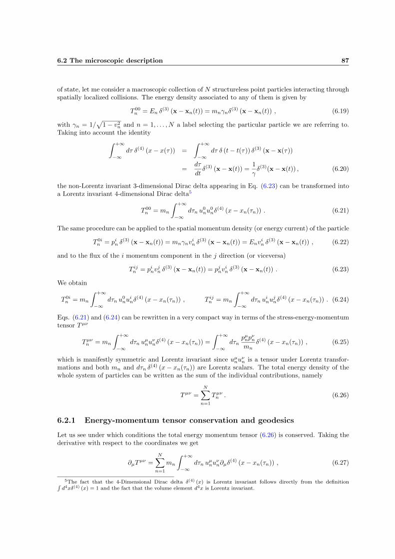
of state, let me consider a macroscopic collection of N structureless point particles interacting throughspatially localized collisions. The energy density associated to any of them is given by

T 00n = En δ

(3) (x− xn(t)) = mnγnδ(3) (x− xn(t)) , (6.19)

with γn = 1/√

1− v2n and n = 1, . . . , N a label selecting the particular particle we are referring to.

Taking into account the identity∫ +∞

−∞dτ δ(4) (x− x(τ)) =

∫ +∞

−∞dτ δ (t− t(τ)) δ(3) (x− x(τ))

=dτ

dtδ(3) (x− x(t)) =

1

γδ(3)(x− x(t)) , (6.20)

the non-Lorentz invariant 3-dimensional Dirac delta appearing in Eq. (6.23) can be transformed intoa Lorentz invariant 4-dimensional Dirac delta5

T 00n = mn

∫ +∞

−∞dτn u

0nu

0nδ

(4) (x− xn(τn)) . (6.21)

The same procedure can be applied to the spatial momentum density (or energy current) of the particle

T 0in = pin δ

(3) (x− xn(t)) = mnγnvin δ

(3) (x− xn(t)) = Envin δ

(3) (x− xn(t)) , (6.22)

and to the flux of the i momentum component in the j direction (or viceversa)

T ijn = pinvjn δ

(3) (x− xn(t)) = pjnvin δ

(3) (x− xn(t)) . (6.23)

We obtain

T 0in = mn

∫ +∞

−∞dτn u

0nu

inδ

(4) (x− xn(τn)) , T ijn = mn

∫ +∞

−∞dτn u

inu

jnδ

(4) (x− xn(τn)) . (6.24)

Eqs. (6.21) and (6.24) can be rewritten in a very compact way in terms of the stress-energy-momentumtensor Tµν

Tµνn = mn

∫ +∞

−∞dτn u

µnu

νnδ

(4) (x− xn(τn)) =

∫ +∞

−∞dτn

pµnpνn

mnδ(4) (x− xn(τn)) , (6.25)

which is manifestly symmetric and Lorentz invariant since uµnuνn is a tensor under Lorentz transfor-

mations and both mn and dτn δ(4) (x− xn(τn)) are Lorentz scalars. The total energy density of the

whole system of particles can be written as the sum of the individual contributions, namely

Tµν =

N∑n=1

Tµνn . (6.26)

6.2.1 Energy-momentum tensor conservation and geodesics

Let us see under which conditions the total energy momentum tensor (6.26) is conserved. Taking thederivative with respect to the coordinates we get

∂µTµν =

N∑n=1

mn

∫ +∞

−∞dτn u

µnu

νn∂µδ

(4) (x− xn(τn)) , (6.27)

5The fact that the 4-Dimensional Dirac delta δ(4) (x) is Lorentz invariant follows directly from the definition∫d4xδ(4) (x) = 1 and the fact that the volume element d4x is Lorentz invariant.

6.2 The microscopic description 88

which using

uµn∂µδ(4) (x− xn(τn)) =

dxµndτn

∂

∂xµδ(4) (x− xn(τn)) = −d/dτnδ(4) (x− xn(τn)) , (6.28)

can be written as

∂µTµν = −

N∑n=1

mn

∫ +∞

−∞dτn

d

dτn

(uνnδ

(4) (x− xn(τn)))

+

N∑n=1

mn

∫ +∞

−∞dτn u

νnδ

(4) (x− xn(τn)) .

The first term in the right hand side of the previous expression disappears in the particles are stable,i.e. if the orbits are closed or come from negative infinite time and disappear into positive infinitetime. We are left then with the second term, which can be written as

∂µTµν =

N∑n=1

∫ +∞

−∞dτn

dpνndτn

δ(4) (x− xn(τn)) =

N∑n=1

dpνndt

δ(3) (x− xn) , (6.29)

with pνn = mnuνn the 4-momentum of the individual particles. The local energy momentum conser-

vation ∂µTµν = 0 requires the particles to be free. Or in other words, the condition ∂µT

µν = 0 isequivalent to the geodesic equation in Minkowski space-time, dpµn/dτ = 0. This will be also the casein curved spacetime.

6.2.2 The fluid limit

On distances d much larger than the typical mean free path a, the number of particles is large andthe statistical fluctuations about the mean properties of the fluid are expected to be small6. Imaginea comoving observer exploring distances d � a. If the fluid is isotropic7, the average value of theT 0i ∝ u0ui component measured by this observer will be zero since the vector ui points in all possibledirections. In this case, the fluid can be characterized in terms of two quantities: its mean densityand pressure over the volume ∆V = d3

ρ =⟨∑

n

Enδ(3) (x− xn)

⟩∆V

, p =1

3

∑i

⟨∑n

pinvinδ

(3) (x− xn)⟩

∆V. (6.30)

A simple inspection of Eqs. (6.30) reveals that, for standard matter, 0 ≤ p ≤ ρ/3. In any otherreference frame, the energy-momentum tensor for the perfect fluid reads

Tµν(x) = (ρ(x) + p(x))uµ(x)uν(x) + p(x)ηµν , (6.31)

with uµ(x) denoting now the average value of the 4-velocities uµi of the individual particles NR insidethe volume8. The perfect fluid form (6.31) can be used to model very different physical situationsthat often fall into one of the following categories:

1. Non-relativistic matter: For small velocities the dispersion relation En =√m2n + p2

n can beapproximated by En ' mn+p2

n/2mn, which plugged back into (6.30) gives rise to ρ ' mnn+ 32p.

Taking into account that the statistical definition of temperature T is twice the energy possessedby each degree of freedom and assuming a monoatomic gas with 3 kinetic degrees of freedom,we can write T = (2/3)× p2

n/2mn and therefore ρ ' mnn+ 32T .

6Remember that, when we later apply the Equivalence Principle, we will have another scale into play: the scaleL at which the gravitational effects start to be important. If this scale happens to be much larger than the scale d(L� d� a), the mean properties of the fluid can be safely considered as constant over the region.

7i.e if the fluid is perfect.8Note that, when writing uµ(x), ρ(x) and p(x) we are explicitly taking into account that the averages can vary from

one region to another.

6.2 The microscopic description 89

2. Dust: A perfect fluid with zero pressure. p = 0, tµν = 0, Tµν = ρdiag (1, 0, 0, 0).

3. Radiation: A perfect highly relativistic fluid. In this case En ' |pn| � mn and therefore9

ρ ' 3p. The energy momentum for radiation is traceless, T = Tµµ = ηµνTµν = −ρ+ 3p = 0.

A worked-out example: The electromagnetic field

The paradigmatic case of a fluid with a radiation equation of state is the electromagneticfield. To see this explicitly, consider the energy density of the electromagnetic field

T00 =1

2

(E2 + B2

), (6.32)

and write it in the way seen by an observer moving with 4-velocity uµ. The electron fieldseen by that observer is given by

Eµ = Fµνuν . (6.33)

Using this expression we get the following covariant expression for the square of the electricfield

E2 = FµνuνFµρu

ρ . (6.34)

A similar expression for the magnetic field square can be obtained from the explicit ex-pression for the square of the electromagnetic field strength tensor

FµνFµν = −2

(E2 −B2

). (6.35)

We obtain

B2 = FµνuνFµρu

ρ +1

2FµνF

µν . (6.36)

Putting Eqs. (6.34) and (6.36) together, the covariant generalization of the energy density(6.32) becomes

ρ =

(FρµF

ρν −

1

4FρσF

ρσηµν

)uµuν , (6.37)

where we have inserted a factor uµuµ = −1. The work is basically done. The quantity in

parenthesis is the sought-for energy-momentum tensor for the electromagnetic field!

Tµν = FρµFρν −

1

4FρσF

ρσηµν . (6.38)

Exercise• Compute the T 0i in terms of the electric and magnetic fields. Do you recognize the

result?

• Prove that the electromagnetic energy-momentum is symmetric Tµν = Tνµ andtraceless, Tµµ = 0. The electromagnetic field behaves as a fluid with equation ofstate p = 1/3ρ.

9Note that the quantity∑i pinvin in Eq. (6.30) can be written as

∑i pinvin =

∑imγnv

invin =

|pn|2En

, which goes to

|pn| when En ' |pn|.

6.3 Einstein equations: Heuristic derivation 90

6.3 Einstein equations: Heuristic derivation

We have finally all the tools needed to derive the Einstein field equations for the gravitational field. Inthe Poisson equation, the gravitational field is determined by the matter distribution. The relativisticversion of the matter distribution10, the energy-momentum tensor TM

µν , must be somehow equated11

to some tensor Kµν depending of the metric gµν and its first and second derivatives12

Kµν = κ2TMµν , (6.39)

with κ2 a proportionality constant to be determined. But, what tensor? Einstein got the answer tothis question trough a complicated process of intuition, trial and error; superhuman exertions in hisown words. As claimed above, the left-hand side of Eq.(6.39) should contain a second order differentialoperator acting on the metric. We already found some quantities with this property in the previouschapter: the Riemann tensor Rµνρσ and its contractions. The most natural tentative for Kµν wouldbe the Ricci tensor Rµν , since this is the contraction appearing in the Newtonian limit of the geodesicdeviation equation (Ri0i0 = Eii). This was also one of the first trial and error choices of Einstein

Rµν ≈ κ2TMµν . (6.40)

Note however that this choice is inconsistent, since the divergence ∇νRµν of the Ricci tensor is, in gen-eral, different from zero and, according to our minimal coupling prescription, the energy-momentumshould be locally conserved, ∇νTM

µν = 0. Indeed, making use of the Bianchi identity (5.71) we can

write ∇µRµν = 1/2∇νR, which together with the trace of Eq. (6.40), R = κ2gµνTMµν = κ2TM, im-

plies the condition ∇µTM = 0. Since the covariant derivative of the scalar quantity TM is just thepartial derivative, we should necessarily have a constant TM throughout the whole spacetime, whichis highly implausible, since, as we know, TM = 0 for the electromagnetic field and TM > 0 for stan-dard matter. On top of that, Eq. (6.40) hides 10 differential equations for 6 physical unknowns: thecomponents of the metric that cannot be freely changed by performing coordinates transformationsin the 4 coordinates. We have to try harder.

The most general combination of symmetric tensors involving up to two derivatives of the metric is

Kµν = Rµν + agµνR+ Λgµν (6.41)

with a and Λ some unknown constants to be determined13. Imposing the local conservation of theenergy-momentum tensor ∇µTM

µν=0 in Eq. (6.39) we get

∇µKµν = ∇µ (Rµν + agµνR) = 0 , (6.42)

where we have taken into account that the covariant derivative ∇µ is metric compatible and therefore∇µ (Λgµν) = 0. Our situation now is much better than that of Einstein, we are aware of the contractedform of the Bianchi identities14 (5.71) and know the precise value of a that satisfies Eq. (6.42), namelya = 1/2. Taking this into account, we can rewrite Eq. (6.39) as

Gµν + Λgµν = κ2TMµν , (6.43)

with

Gµν ≡ Rµν −1

2gµνR , (6.44)

10Matter should be understood in a broad sense, meaning really matter, radiation etc. . .11A relativistic generalization should take the form of an equation between tensors.12The requirement of having derivatives only up to second order is certainly reasonable. If this were not the case, one

would have to specify for the Cauchy problem not only the value of the metric and its first derivative, but also higherderivatives on a spacelike surface.

13A possible proportionality constant in front of Rµν has been factored out and incorporated in the still unknownfactors κ and Lambda in the right hand side of Eq. (6.39).

14He wasn’t.

6.3 Einstein equations: Heuristic derivation 91

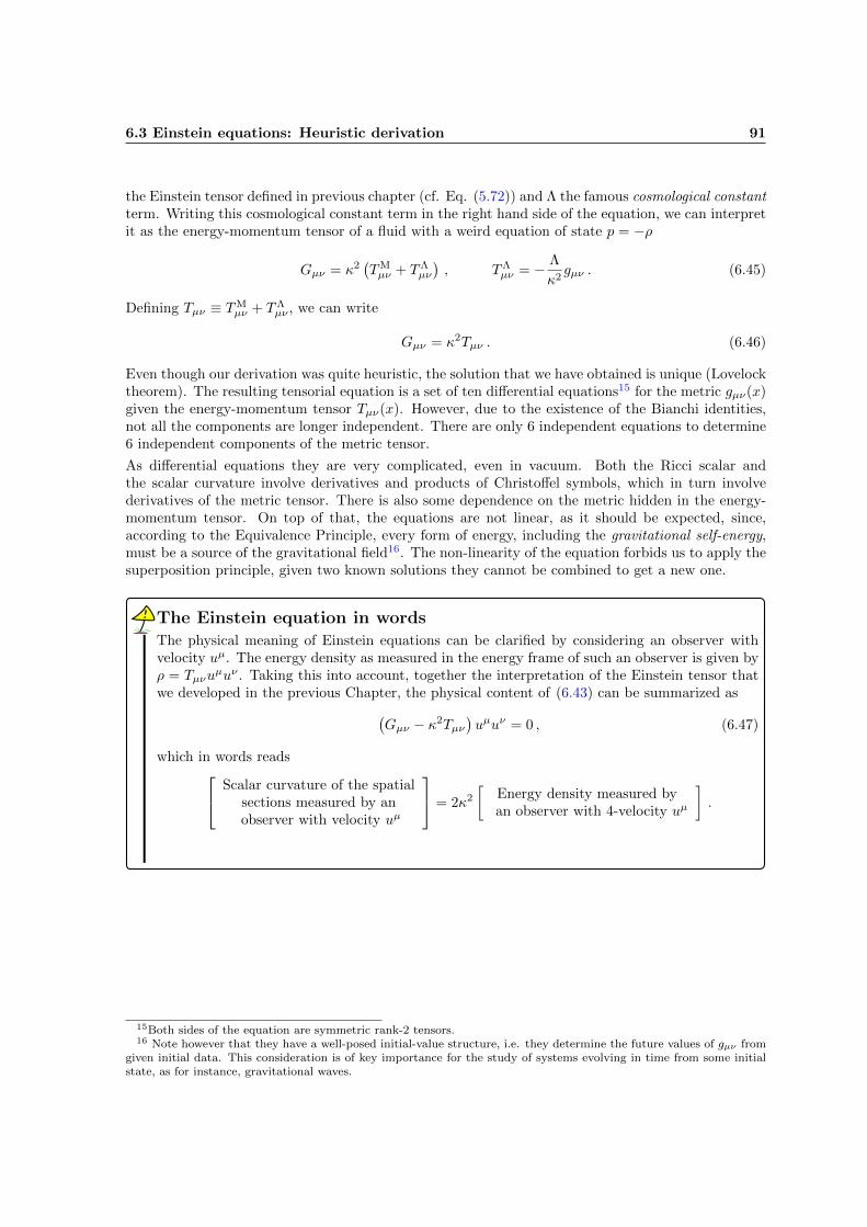
the Einstein tensor defined in previous chapter (cf. Eq. (5.72)) and Λ the famous cosmological constantterm. Writing this cosmological constant term in the right hand side of the equation, we can interpretit as the energy-momentum tensor of a fluid with a weird equation of state p = −ρ

Gµν = κ2(TMµν + TΛ

µν

), TΛ

µν = − Λ

κ2gµν . (6.45)

Defining Tµν ≡ TMµν + TΛ

µν , we can write

Gµν = κ2Tµν . (6.46)

Even though our derivation was quite heuristic, the solution that we have obtained is unique (Lovelocktheorem). The resulting tensorial equation is a set of ten differential equations15 for the metric gµν(x)given the energy-momentum tensor Tµν(x). However, due to the existence of the Bianchi identities,not all the components are longer independent. There are only 6 independent equations to determine6 independent components of the metric tensor.

As differential equations they are very complicated, even in vacuum. Both the Ricci scalar andthe scalar curvature involve derivatives and products of Christoffel symbols, which in turn involvederivatives of the metric tensor. There is also some dependence on the metric hidden in the energy-momentum tensor. On top of that, the equations are not linear, as it should be expected, since,according to the Equivalence Principle, every form of energy, including the gravitational self-energy,must be a source of the gravitational field16. The non-linearity of the equation forbids us to apply thesuperposition principle, given two known solutions they cannot be combined to get a new one.

The Einstein equation in wordsThe physical meaning of Einstein equations can be clarified by considering an observer withvelocity uµ. The energy density as measured in the energy frame of such an observer is given byρ = Tµνu

µuν . Taking this into account, together the interpretation of the Einstein tensor thatwe developed in the previous Chapter, the physical content of (6.43) can be summarized as(

Gµν − κ2Tµν)uµuν = 0 , (6.47)

which in words reads Scalar curvature of the spatialsections measured by anobserver with velocity uµ

= 2κ2

[Energy density measured byan observer with 4-velocity uµ

].

15Both sides of the equation are symmetric rank-2 tensors.16 Note however that they have a well-posed initial-value structure, i.e. they determine the future values of gµν from

given initial data. This consideration is of key importance for the study of systems evolving in time from some initialstate, as for instance, gravitational waves.

6.4 The linearized theory of gravity 92

Newton Einstein

Newton 2nd law Geodesic equation

d2xi

dt2 = −δij ∂Φ∂xj

d2xµ

d2σ = −Γµνρ∂xρ

dσdxν

dσ

Tidal deviation Geodesic deviation

d2ξi

dt2 = −Eij ξj D2ξµ

dσ2 = −Rµνρσuνuσξρ

1st Bianchi identity 1st Bianchi identitiy

Eij = Eji Rµνρσ +Rµρσν +Rµσνρ = 0

2nd Bianchi identity 2nd Bianchi identitiy

Ei[j,l] = 0 ∇κRµνρσ +∇σRµνκρ +∇ρRµνσκ = 0

mass density Energy-momentum tensor

ρ Tµν

Poisson equation Einstein equation

Eii = 4πGρ Gµν = 8πGTµν

single elliptic equation 10 coupled equations

4 elliptic and 6 hyperbolic

boundary data required initial and boundary data required

Table 6.1: Newtonian vs Einstenian description of gravity.

6.4 The linearized theory of gravity

Equation (6.46) looks very promising but we have still to prove that it is able to reproduce theNewtonian theory of gravity and determine the value of the unknown constants κ and Λ. The fastestway to obtain the Newtonian limit is to use the assumptions discussed in Section 3.6. Let me howeverrelax these assumptions and obtain the general expression for the Einstein equation in the so-calledweak field limit. This limit is defined by the condition

gµν = ηµν + hµν , with |hµν | � 1 . (6.48)

The quantity hµν is then understood as a small perturbation on top of the Minkowski background.Consistently with this point of view, we will raise and lower its indices with the flat Minkowski metricηµν , namely hµσ = ηµρhρσ , h

µν = ηνσhµσ .

In order to compute the expression for the Einstein tensor Gµν at the lowest order in perturbation

6.4 The linearized theory of gravity 93

theory we must first determine the linearized version of the Ricci tensor and the scalar curvature,which are functions of the metric connection Γµνρ. Inserting the expansion (6.48) into the definitionof the metric connection, we get

Γµνρ =1

2ηµσ (∂νhσρ + ∂ρhσν − ∂σhρν) +O(h2

µν) . (6.49)

The next step is to compute the 4 pieces of Riemman tensor, which, written in a very schematic way,have the structure R······ ∼ ∂Γ − ∂Γ + ΓΓ + ΓΓ. Taking into account (6.49), we realize that only thefirst two terms (∼ ∂Γ) give a contribution to the leading order

Rµνρσ =1

2∂ρ (∂σh

µν + ∂νh

µσ − ∂µhνσ)− (ρ↔ σ) =

1

2(∂ν∂ρh

µσ + ∂σ∂

µhνρ − (ρ↔ σ)) . (6.50)

The linearized version of the Ricci tensor and the scalar of curvature can be computed by simplyperforming contractions in the previous expression. Denoting respectively by h ≡ hµµ and 2 = ∂µ∂µthe trace of the perturbation tensor and the d’Alambertian operator and contracting the indices µand σ in Eq. (7.17), we get17

Rνρ = −1

2(2hνρ + ∂ν∂ρh− ∂ν∂σhσρ − ∂ρ∂σhσν) , (6.51)

which can be further contracted in the indices ν and ρ to obtain

R = Rνν = ηνρRνρ = −2h+ ∂ν∂σhνσ . (6.52)

Collecting all the terms and inserting them into the definition of the Einstein tensor (6.44), we get

Gνρ = −1

2(∂ν∂ρh+ 2hνρ − ∂ν∂σhσρ − ∂ρ∂σhσν − ηνρ2h+ ηνρ∂µ∂σh

µσ)

= −1

2

(2hνρ + ηνρ∂µ∂σh

µσ − ∂ν∂σhσρ − ∂ρ∂σhσν), (6.53)

where in the last step we have defined the so-called trace reverse

hµν ≡ hµν −1

2ηµνh , hµν = hµν −

1

2ηµν h , (6.54)

which keeps track of the extra terms obtained when passing from Rνρ to Gνρ. The name trace reverse

comes from the property h ≡ hµµ = −h. Note also the useful properties

˜hµν = hµν , Gµν = Rµν . (6.55)

The linearized Einstein equations becomes finally(2hνρ + ηνρ∂µ∂σh

µσ − ∂ν∂σhσρ − ∂ρ∂σhσν)

= −2κ2Tνρ . (6.56)

The resulting expression is rather involved, but fortunately we still have some freedom to play with:the gauge freedom.

17The global minus sign comes from the permutation of the last two indices two construct the Ricci scalar.

6.4 The linearized theory of gravity 94

Gauge fixing

Eqs. (7.17) and (6.53), and therefore (6.56), are invariant under the transformation

hνρ −→ hνρ − ∂νξρ − ∂ρξν , (6.57)

as can be easily verified be performing the explicit computation. This kind of change iscalled a gauge transformation, due to the strong analogy with the gauge transformations inthe electromagnetic theory. The simplest way to understand this gauge freedom is to traceit back to the transformation of the full metric gµν . Consider an infinitesimal transformationxµ → xµ = xµ + ξµ. Under such a transformation the metric changes to

gµν (xρ + ξρ) = gρσ(xρ)∂xµ

∂xρ∂xν

∂xσ(6.58)

= gρσ (δµρ + ∂ρξµ) (δνσ + ∂σξ

ν)

= gµν(xρ) + gµσ∂σξν + gνρ∂ρξ

µ .

Expanding the left-hand side of this equation in a Taylor series in ξρ and retaining only theterms up to linear order, we get

gµν(xρ) = gµν(xρ) + δgµν , (6.59)

withδgµν ≡ −ξρ∂ρgµν + gµρ∂ρξ

ν + gνρ∂ρξµ = ∇νξµ +∇µξν . (6.60)

In the particular case in which the perturbation is performed around the Minkowski background,gµν = hµν + ηµν , the covariant derivatives in (6.59) become standard derivatives and we recoverthe transformation law (6.57). The linearized theory is invariant under (6.57) because thefull nonlinear theory is invariant under general coordinate transformations! This is extremelyinteresting, since it allows us to further simplify the linearized version of the Einstein tensor bysimply performing infinitesimal coordinates transformations, or in other words, changes froma splitting gµν = ηµν + hold to a different splitting gµν = ηµν + hnew. A simple inspection ofEq. (6.56) reveals that an interesting condition to be satisfied by the trace reverse tensor inthe new coordinate system would be the tensor analog of the Lorenz gauge ∂µA

µ = 0 in theelectromagnetic theorya, namely

∂ρhνρnew = 0 . (6.61)

Let us see if we are allowed to choose such a gauge. The change in the trace reverse tensor hµνfollows directly from Eqs. (6.54) and (6.57)

hνρnew = hνρold − ∂νξρ − ∂ρξν + ηνρ∂µξ

µ . (6.62)

Taking the derivative of this equation we get

∂ρhνρnew = ∂ρh

νρold −2ξν . (6.63)

In order to satisfy the gauge fixing (6.61), ξν must be a solution of the inhomogeneous waveequation

2ξν = ∂ρhνρold . (6.64)

The existence of a solution transforming from an arbitrary hµν to the so-called Lorenz gauge

∂ρhνρnew = 0 is guaranteedb for sufficiently well behaved ∂ρh

νρold. In fact, the choice is not unique

since we can always add to it any solution of the homogeneous wave equation 2ξνH = 0 and the

result will still obey 2 (ξν + ξνH) = ∂ρhνρold. The Lorenz gauge ∂ρh

νρnew = 0 is actually a set of

gauges.

aIt “kills” three of the four terms in (6.53).bAs you learnt in your electrodynamic course, the solution of this equation can be obtained by means of the

retarded Green functions of the d’Alambertian operator.

6.4 The linearized theory of gravity 95

x'

x

x- x'

P

O

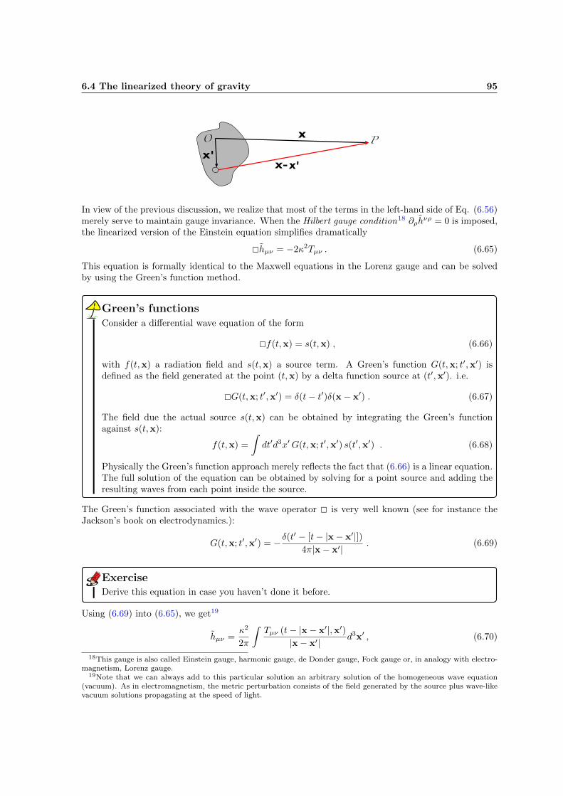
In view of the previous discussion, we realize that most of the terms in the left-hand side of Eq. (6.56)merely serve to maintain gauge invariance. When the Hilbert gauge condition18 ∂ρh

νρ = 0 is imposed,the linearized version of the Einstein equation simplifies dramatically

2hµν = −2κ2Tµν . (6.65)

This equation is formally identical to the Maxwell equations in the Lorenz gauge and can be solvedby using the Green’s function method.

Green’s functionsConsider a differential wave equation of the form

2f(t,x) = s(t,x) , (6.66)

with f(t,x) a radiation field and s(t,x) a source term. A Green’s function G(t,x; t′,x′) isdefined as the field generated at the point (t,x) by a delta function source at (t′,x′). i.e.

2G(t,x; t′,x′) = δ(t− t′)δ(x− x′) . (6.67)

The field due the actual source s(t,x) can be obtained by integrating the Green’s functionagainst s(t,x):

f(t,x) =

∫dt′d3x′G(t,x; t′,x′) s(t′,x′) . (6.68)

Physically the Green’s function approach merely reflects the fact that (6.66) is a linear equation.The full solution of the equation can be obtained by solving for a point source and adding theresulting waves from each point inside the source.

The Green’s function associated with the wave operator 2 is very well known (see for instance theJackson’s book on electrodynamics.):

G(t,x; t′,x′) = −δ(t′ − [t− |x− x′|])

4π|x− x′|. (6.69)

ExerciseDerive this equation in case you haven’t done it before.

Using (6.69) into (6.65), we get19

hµν =κ2

2π

∫Tµν (t− |x− x′|,x′)

|x− x′|d3x′ , (6.70)

18This gauge is also called Einstein gauge, harmonic gauge, de Donder gauge, Fock gauge or, in analogy with electro-magnetism, Lorenz gauge.

19Note that we can always add to this particular solution an arbitrary solution of the homogeneous wave equation(vacuum). As in electromagnetism, the metric perturbation consists of the field generated by the source plus wave-likevacuum solutions propagating at the speed of light.

6.4 The linearized theory of gravity 96

which is analogous to the relation between the vector potential Aµ and the current Jµ in electromag-netism. Note the argument t − |x − x′| = t − |x − x′|/c. Eq. (6.70) is a retarded solution20, takinginto account the lag associated with the propagation of information from events at x to position x′.Gravitational influences propagate at the finite speed of light. Action at a distance is gone forever!We will be back to this point at the next chapter , but before let me finish our main task: determiningthe value of the constants κ2 and Λ. For doing that let me consider the case we know better: the grav-itational field created by a static spherical mass distribution of total mass M . The energy-momentumtensor for such a system has only one non-vanishing component (cf. Eq. (6.45))

T 00 =

(ρ+

Λ

κ2

)diag (1, 0, 0, 0) . (6.72)

Plugging this into the time independent version of Eq. (6.70), we get

h00 =κ2

2π

∫ρ (x′)

|x− x′|d3x′ +

1

2π

∫Λ

|x− x′|d3x′ , h0i = 0 , hij = 0 . (6.73)

If the mass distribution is concentrated around the origin (x′ = 0), the component h00 evaluated at adistance r = |x− x′| becomes21

h00 =κ2

2π

∫ρ (x′)

rd3x′ +

1

2π

∫Λ

rd3x′ =

κ2

2π

M

r+

2

3Λr2 (6.74)

with

M =

∫ρ (x′) d3x′ (6.75)

the total mass of our spherical distribution. Taking now into account that h = ηµν hµν = −h00 andusing the definition (6.54) we get

h00 = h11 = h22 = h33 =κ2M

4πr+

1

3Λr2 . (6.76)

Comparing this result with that obtained by performing the weak field limit of the geodesic equation inthe Λ = 0 case, hΛ=0

00 = −2Φ = 2GM/r, allows us to identify the sought-for proportionality constant

κ2 = 8πG . (6.77)

When Λ 6= 0, the Newtonian potential becomes modified at long distances

Φ = −GMr− Λ

6r2 (6.78)

and line element takes the form

ds2 = −(

1− 2GM

r− 1

3Λr2

)dt2 +

(1 +

2GM

r+

1

3Λr2

)dX2 , (6.79)

with dX2 ≡ dx2 + dy2 + dz2. In Newtonian terms, a positive cosmological constant (Λ > 0) gives riseto a repulsive force per unit mass whose strength increases linearly with the distance

f = −GMr2

ur +Λ

3r ur , (6.80)

20The retarded solution is obtained by imposing the Kirchoff-Sommerfeld “no-incoming radiation” boundary conditionat past null infinity

limt→∞

(∂r + ∂t) (rhµν) = 0 , (6.71)

with the limit taken along any surface with ct + r =constant, together with the condition that rhµν and r∂ρhµν arebounded in this limit.

21Note that the integral in over the prime variables!

6.4 The linearized theory of gravity 97

Cosmological constant

If Λ 6= 0, it must be at least very small, ρΛ � ρmatter, to avoid any observational effect inthose situations in which the Newton’s theory of gravity successfully explains the observations.Taking into account, for instance, that we do not see any modification of the Newtonian theoryof gravity within the solar system, we can set the limit

|ρΛ| =|Λ|

8πG≤ ρSolar −→ |ρΛ| ≤

3M�4πR3

Pluto

' 10−29 GeV4 (6.81)

which, as assumed, makes the contribution of Λ completely negligible on the scale of the systemswe will be interested in in this coursea .

aIt will play however a fundamental role at larger scales, as those you will considered in your Cosmologycourse.

Linearized Gravity Electromagnetism

Field equation Einstein equation with Maxwell equations

gµν = hµν + hµν

Basic potentials Linearized metric 4-vector potential

hµν(x) Aµ = (Φ,A)

Sources Energy-momentum tensor 4-vector current

Tµν Jµ = (ρ,J)

Lorenz gauge ∂µhµν = 0 ∂µA

µ = 0

hµν = hµν − 12ηµνh

Sourced wave equation 2hµν = −16πGTµν 2Aµ = Jµ

Solution hµν = 4G∫ [Tµν ]ret|x−x′| d

3x′ Aµ = 14π

∫ [Jµ]ret|x−x′|d

3x′

Table 6.2: Linearized Einstein equations vs Maxwell equations.