SMATS 2040 MTP 5-1

Chapter 5

Urban Area Travel Demand Modeling Process and Results

Because of the interaction of traffic between Saginaw, Bay City and Midland it was decided that the travel patterns of the area could be better modeled if a regional model was built. The travel demand model used for the Saginaw Area Transportation Study (SMATS) 2040 Metropolitan Transportation Plan (MTP) is a regional model, referred to as the Great Lakes Bay Region (GLBR) Model that includes Saginaw, Bay and Midland Counties. This effort required coordination and cooperation between Saginaw Metropolitan Area Transportation Study (SMATS), Bay City Area Transportation Study (BCATS), Midland County Road Commission and the City of Midland. The urban area travel demand modeling process for the Saginaw County portion of the GLBR Model was a cooperative effort between the Saginaw Metropolitan Area Transportation Study (SMATS), being the Metropolitan Planning Organization (MPO), and the Michigan Department of Transportation, Statewide and Urban Travel Analysis Section (MDOT). MDOT provided the lead role in the process and assumed responsibility for modeling activities with both entities reaching consensus on selective process decisions. The local transportation planning agency is the MPO, comprised of representatives of local governmental units and is the umbrella organization responsible for carrying out transportation planning in cooperation with MDOT and the Federal Highway Administration. This is typically accomplished by full coordination of the local agencies with the MPO. The results of the modeling effort is to provide an important decision making tool for the MPO Metropolitan Transportation Plan development as well as any transportation related studies that might follow. The modeling process is a systems-level effort. Although individual links of a highway network can be analyzed, the results are intended for determination of system-wide impacts. At the systems level, impacts are assessed on a broader scale than the project level. The travel demand modeling for SMATS has been completed through the use of TransCAD software utilized by MDOT. The model is a computer estimation of current and future traffic conditions and is a system-level transportation planning model. Capacity deficiencies are determined using a Level of Service D capacity. The urban travel demand forecasting process used has seven phases:

SMATS 2040 MTP 5-2

1. Data Collection, in which socio-economic and facility inventory data are collected.

2. Trip Generation, which calculates the number of person trips produced in or

attracted to a traffic analysis zone (TAZ). 3. Trip Distribution, which takes the person trips produced in a TAZ and

distributes them to all other TAZs, based on attractiveness of the zone. 4. Mode Choice, which assigns person trips to a mode of travel such as drive

alone, shared ride 2, shared ride 3+, walk to transit, park and ride transit. 5. Assignment, which determines what routes are utilized for trips. There is a

highway assignment and a transit assignment. 6. Model Calibration/Validation, which is performed at the end of each

modeling step to make sure that the results from that step are within reasonable ranges. The final assignment validation involves verifying that the volumes (trips) estimated in the base year traffic assignment replicate observed traffic counts.

7. System Analysis, tests alternatives and analyzes changes in order to

improve the transportation system. There are two basic systems of data organization in the travel demand forecasting process. The first system of data is organized based on the street system. Roads with a national functional class (NFC) designation of "minor collector" and higher are included in the network. Some local roads are included to provide connectivity in the network or because they were deemed regionally significant. The unit of analysis is called a "link." Usually, a link is a segment of roadway which is terminated at each end by an intersection. In a traffic assignment network, intersections are called "nodes." Therefore, a link has a node at each end. The second data organization mechanism is the Traffic Analysis Zones (TAZ). TAZs are determined based upon several criteria, including similarity of land use, compatibility with jurisdictional boundaries, the presence of physical boundaries, and compatibility with the street system. Streets are generally utilized as zone boundary edges. All socio-economic and trip generation information for both the base year and future year are summarized by TAZ. The Traffic Analysis Zones used for model development are depicted on a series of maps that are on file with the MPO and available for viewing at the SMATS office. They have not been reproduced here due to space limitations.

SMATS 2040 MTP 5-3

The two data systems, the street system (network) and the TAZ system (socio-economic data), are interrelated through the use of "centroids." Each TAZ is represented on the network by a point (centroid) which represents the weighted center of activity for that TAZ. A centroid is connected by a set of links to the adjacent street system. That is, the network is provided with a special set of links for each TAZ which connects the TAZ to the street system. Since every TAZ is connected to the street system by these "centroid connectors,” it is possible for trips from each zone to reach every other zone by way of a number of paths through the street system.

Network A computerized "network" (traffic assignment network) is built to represent the existing street system. The GLBR Model network is based on the Michigan Geographic Framework version 10 and includes most streets within the study area classified as a "minor collector" or higher by the national functional classification system. Other roads are added to provide continuity and/or allow interchange between these facilities. Transportation system information or network attributes required for each link include facility type, area type, lane width, number of through lanes, parking available, national functional classification, traffic counts (where available), and volumes for level of service D (frequently described as its capacity). If the information is not the same for the entire length of a link, the predominant value is used. The network attributes were provided to the MPO and MDOT staff by the respective road agencies, with the exclusion of link capacity. The link capacity was determined by utilizing the Capacity Calculator program which takes into account the network attributes and sets a capacity that would approximate a level of service “D” or acceptable level of traffic. Higher volume to capacity ratios are characterized by: stop-and–go-travel, reduced flow rates and severe intersection delays. This typifies unacceptable or deficient traffic conditions. The street network is used in the traffic assignment process. The traffic assignment process takes the trip interactions between zones from trip distribution and loads them onto the network. The travel paths for each zone-to-zone interchange are based on the minimum travel time between zones. They are calculated by a computer program which examines all possible paths from each origin zone to all destination zones. The shortest path is determined by the distance of each link and the speed at which it operates. The program then calculates travel times for all of the possible paths between centroids and records the links which comprise the shortest travel time path.

SMATS 2040 MTP 5-4

The transit network is used in the transit assignment process and overlays the street network as a route system. It reflects the current fixed route system available for the base year. It has its own set of attributes such as bus headway, speed and rider fee. Person trips that are determined to be transit trips are assigned to this network. Speeds used to calculate minimum travel times are based on each link's national functional classification, facility type, and area type. Speeds represent a relative impedance to travel and not posted speed limits.

Socio-Economic Data Travel demand models are driven, in part, by the relationship of land use activities and characteristics to the transportation network. Specific inputs to the modeling process are land use activity including the number of households, population-in-households, vehicles, and employment located in a given transportation analysis zone (TAZ). The modeling process translates this data into vehicle trips on the modeled transportation network. Socio-Economic data were developed for the 2009 base year and for the 2020, 2030 and 2040 forecast years. It is important to remember that socio-economic forecasting is essentially a matter of judgment. Judgment is required in selecting the type of forecast to be implemented; in determining the procedures for making the forecast; and, the process used in reviewing the effects of the factors that induce changes in population and employment. The establishment of a large new industry or the loss of a similar size industry can lead to considerable impact on an area’s development. Therefore, although socio-economic projections are a useful and required tool in the planning of an area’s future growth and development, it is important to note that the projections are not infallible and should be modified as time progresses to better reflect development impacts occurring in the SMATS planning area. The TAZ’s were created from the 2000 census blocks and constrained by the network and Minor Civil Division (MCD) boundaries. Values for population and occupied households were aggregated from the 2000 census blocks to arrive at TAZ totals for 2000. MPO staff used this and MCD projections as well as input from local officials to develop the TAZ values for the base year of 2009 and forecast years of, 2020, 2030 and 2040. Employment data was obtained from the combination of the Michigan Employment Security Commission (MESC), and the propriety databases

SMATS 2040 MTP 5-5

available from Claritas (2008 Business Point Data) and Hoovers (business address file). The resulting database was reviewed locally. The employment data for 2009, 2020, 2030 and 2040 were developed using growth rates based on the REMI (Regional Econometric, Inc.) projections as well as local knowledge of expected development. SMATS staff and committees reviewed the estimates and projections and made adjustments given their local knowledge and greater understanding of the unique local circumstances in each TAZ.

Trip Generation The trip generation process calculates the number of person-trips produced from or attracted to a zone, based on the socio-economic characteristics of that zone. The urban transportation forecasting models do not consider travel characteristics such as direction, length, or time of occurrence as part of trip generation. The relationship between person-trip making and land activity are expressed in equations for use in the modeling process. The formulas were derived from MI Travel Counts Michigan travel survey data and other research throughout the United States. Productions were generated with a cross-classification look-up process based on household demographics. Attractions were generated with a regression approach based on employment and household demographics. In order to develop a trip table, productions (P's) and attractions (A's) must be balanced also referred to as normalization. The GLBR travel demand model also has a simple truck model that estimates commercial and heavy truck traffic based on production and attraction relationships developed from the Quick Response Freight Manual I (QRFM I). The QRFM I uses the employment data from the TAZs in its calculations. Trips that begin or end beyond the study area boundary are called "cordon trips." These trips are made up of two components: external to internal (EI) or internal to external (IE) trips and through-trips (EE). EI trips are those trips which start outside the study area and end in the study area. IE trips start inside the study area and end outside the study area. EE trips are those trips that pass through the study area without stopping; this matrix is referred to as the through-trip table.

Trip Distribution Trip distribution involves the use of mathematical formula which determines how many of the trips produced in a zone will be attracted to each of the other zones. It connects the ends of trips produced in one zone to the ends of trips attracted to other zones. The equations are based on travel time between zones

SMATS 2040 MTP 5-6

and the relative level of activity in each zone. Trip purpose is an important factor in development of these relationships. The trip relationship formula developed in this process is based on principals and algorithms commonly referred to as the Gravity Model. The process which connects productions to attractions is called trip distribution. The most widely used and documented technique is the "gravity model" which was originally derived from Newton's Law of Gravity. Newton's Law states that the attractive force between any two bodies is directly related to the masses of the bodies and inversely related to the distance between them. Analogously, in the trip distribution model, the number of trips between two areas is directly related to the level of activity in an area (represented by its trip generation) and inversely related to the distance between the areas (represented as a function of travel time). Research has determined that the pure gravity model equation does not adequately predict the distribution of trips between zones. In most models the value of time for each purpose is modified by an exponentially determined "travel time factor" or "F factor" --also known as a "Friction Factor." "F factors" represent the average area-wide effect that various levels of travel time have on travel between zones. The "F factors" used were developed using an exponential function described in the Travel Estimation Techniques for Urban Planning, NCHRP 365. The matrix is generated in TransCAD during the gravity model process. The primary inputs to the gravity model are the normalized productions (P’s) and attractions (A's) by trip purpose developed in the trip generation phase. The second data input is a measure of the temporal separation between zones. This measure is an estimate of travel time over the transportation network. Zone-to-zone travel times are referred to as "skims." In order to more closely approximate actual times between zones and also to account for the travel time for intra-zonal trips, the skims were updated to include terminal and intra-zonal times. Terminal times account for the non-driving portion of each end of the trip and were generated from a look-up table based on area type. They represent that portion of the total travel time used for parking and walking to the actual destination. Intra-zonal travel time is the time of trips that begin and end within the same zone. Intra-zonal travel times were calculated utilizing a nearest neighbor routine. The Gravity Model utilizes the by-purpose P’s & A's, the by-purpose "F factors", and the travel times, including terminal and intra-zonal.

SMATS 2040 MTP 5-7

Mode Choice

The number of person trips and their trip starting and ending point have been determined in the trip generation and trip distribution steps. The mode choice step determines how each person trip will travel. The GLBR travel demand model uses a nested logit model to predict mode choice.

With this logit structure the basic modes are: 1. Single Occupancy Vehicle (SOV) 2. Shared Ride 2 people in vehicle (SR2) 3. Shared Ride 3 or more people in vehicle (SR3+) 4. Walk to transit stop 5. Drive to transit stop Mode choice model utility equations are used to predict the mode used for a trip. Utility equations vary by trip type and take into consideration things like in-vehicle time, out-of-vehicle time, length and cost. The proximity to transit routes or park and ride locations limits the TAZs that can utilize transit options. The output to this step is a vehicle trip matrix and transit trip matrix. The external trips and the truck trips are added to the vehicle trip matrix.

Assignment The GBLR model has 4 time periods that were developed to match the peak periods observed in traffic counts. The following period were used: AM Peak (7a - 9a) Mid Day (9a - 3p) PM Peak (3p - 6p) Night Time (6p – 7a) A fixed time of day factor method was utilized. The factors were developed from the MI Travel Counts Michigan travel survey data and vary by trip type. Default factors from the Quick Response Freight Manual I (QRFM I) were used for truck trips.

SMATS 2040 MTP 5-8

The traffic assignment process takes the trips produced in a zone (trip generation) and distributed to other zones (trip distribution) and loads them onto the network via the centroid connectors. A program examines all of the possible paths from each zone to all other zones and calculates all reasonable time paths from each zone (centroid) to all other zones. Trips are assigned to paths that are the shortest path between each combination of zones. As the volumes assigned to links approach capacity, travel times on all paths are recalculated to reflect the congestion and the remaining trips are assigned to the next shortest path. This process continues through several iterations until no trip can reduce its travel time by taking the next shortest path. This is a user equilibrium assignment method and reflects the alternative routes that motorists use as the shortest path becomes congested. The assignment produces an assigned volume for each link. The transit assignment is a daily assignment and uses the transit network route system to assign the shortest path for trips.

Model Calibration/Validation The outputs of each of the four main steps, Trip Generation, Trip distribution, Mode Choice and Assignment, are checked for reasonableness against national standards. Modifications can be made at each step before moving on to the next. The final model calibration/validation verifies that the assigned volumes simulate actual traffic counts on the street system. When significant differences occur, additional analysis is conducted to determine the reason. At this time additional modifications may be made to the network speeds and configurations (hence paths), trip generation (special generators), trip distribution (F factors), socio-economic data, or traffic counts. The purpose of this model calibration phase is to verify that the base year assigned volumes from the traffic assignment model simulate actual base year traffic counts. When this step is completed, the systems model is considered statistically acceptable. This means that future socio-economic data or future network capacity changes can be substituted for base (existing) data. The trip generation, trip distribution, mode choice and traffic assignment steps can be repeated, and future trips can be estimated for systems analysis. It is assumed that the quantifiable relationships modeled in the base year will remain reasonably stable over time.

Applications of the Calibrated/Validated Model Forecasted travel is produced by substituting forecasted socio-economic and transportation system data for the base year data. This forecasted data is

SMATS 2040 MTP 5-9

provided by the MPO. The same mathematical formulae are used for the base and future year data. The assumption is made that the relationships expressed by the formulae in the base year will remain constant over time (to the target date). After either base year or future trips are simulated, other types of modeling studies can be conducted.

• Network alternatives to relieve congestion can be tested for the 2040 Metropolitan Transportation Plan. Future traffic can be assigned to the existing network to show what would happen in the future if no improvements were made to the present transportation system. This process is often referred to as "deficiency analysis." From this, improvements can be planned that would alleviate demonstrated capacity problems.

• The impact of planned roadway improvements or network changes can be

assessed.

• Links can be analyzed to determine what zones are contributing to the travel on that link. This can be shown as a percentage breakdown of total link volume.

• The network can be tested to simulate conditions with or without a

proposed bridge or new road segment. The assigned future volumes on adjacent links would then be compared to determine traffic flow impacts. This, in turn, would assist in assessing whether the bridge should be replaced and/or where it should be relocated.

• Road closure/detour evaluation studies can be conducted to determine

the effects of closing a roadway. This type of study is very useful for construction management.

• The impacts of land use changes on the network can also be evaluated

(e.g., what are the impacts of a new regional mall being built). Two issues are critical in using the modeling tools and processes:

• The modeling process is most effective for system level analysis. Although detailed volumes for individual intersection and "links" of a highway are an output of the model, additional analysis and modification of the model output may be required for project level analysis.

• The accuracy of the model is heavily dependent on the accuracy of the

SMATS 2040 MTP 5-10

socio-economic data and network data provided by the local participating agencies, and the skill of the users in interpreting the reasonableness of the results.

System Analysis for MTP Generally three different alternative scenarios are developed for the Long Range Transportation Plan: 1. Existing trips on the existing system. This is the "calibrated," existing

network/scenario. This is a prerequisite for the other two scenarios. 2. Future trips on the existing network. Future trips are assigned to the

existing network. This alternative displays future capacity and congestion problems if no improvements to the system are made. This is called the "No Build" alternative, and usually includes the existing system, plus any projects which are committed to be built in the future.

3. Future trips on the future system. This scenario is the future Metropolitan

Transportation Plan network. It includes capacity projects listed in the MTP.

It is important to remember that the volume to capacity ratio reflects a volume for a specified time period and a capacity for that same period of time. It does not reflect deficiencies that only occur briefly at certain short time periods or because of roadway geometrics, or roadway condition. A series of maps was developed to display system deficiencies for the 2009 base year, 2040 with no capacity projects built, and 2040 with the capacity projects identified in the plan. For each scenario, separate maps were generated for each of the time periods considered: A.M. Peak, Mid-Day, P.M. Peak, and Night. Electronic copies of the full set of maps are on file with the MPO. To keep the electronic plan document a reasonable size, only the daily deficiency maps are included at the end of this chapter. These maps are composites that include the deficiencies from all the time periods on a single map for the 2009, 2040 “no build” and 2040 “build” scenarios. Finally, the deficiencies identified in the modeling process are also listed in Table 5-1.

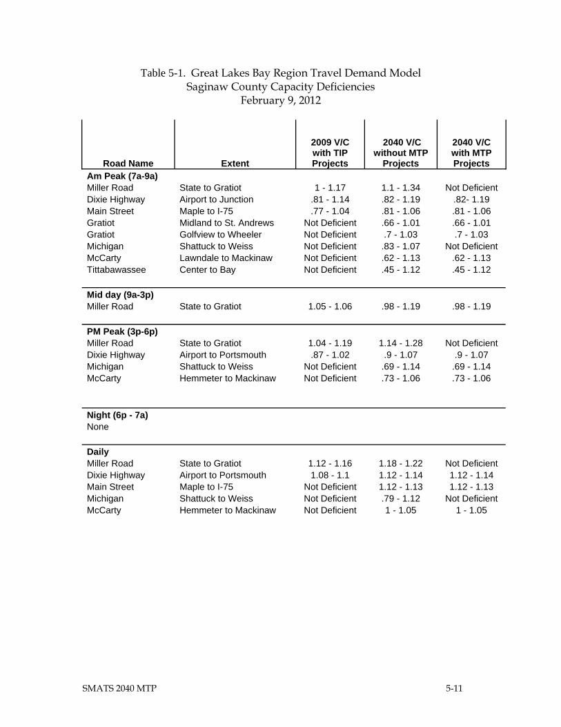
SMATS 2040 MTP 5-11

Table 5-1. Great Lakes Bay Region Travel Demand Model Saginaw County Capacity Deficiencies

February 9, 2012

Road Name Extent

2009 V/C with TIP Projects

2040 V/C without MTP

Projects

2040 V/C with MTP Projects

Am Peak (7a-9a) Miller Road State to Gratiot 1 - 1.17 1.1 - 1.34 Not Deficient Dixie Highway Airport to Junction .81 - 1.14 .82 - 1.19 .82- 1.19 Main Street Maple to I-75 .77 - 1.04 .81 - 1.06 .81 - 1.06 Gratiot Midland to St. Andrews Not Deficient .66 - 1.01 .66 - 1.01 Gratiot Golfview to Wheeler Not Deficient .7 - 1.03 .7 - 1.03 Michigan Shattuck to Weiss Not Deficient .83 - 1.07 Not Deficient McCarty Lawndale to Mackinaw Not Deficient .62 - 1.13 .62 - 1.13 Tittabawassee Center to Bay Not Deficient .45 - 1.12 .45 - 1.12 Mid day (9a-3p) Miller Road State to Gratiot 1.05 - 1.06 .98 - 1.19 .98 - 1.19 PM Peak (3p-6p) Miller Road State to Gratiot 1.04 - 1.19 1.14 - 1.28 Not Deficient Dixie Highway Airport to Portsmouth .87 - 1.02 .9 - 1.07 .9 - 1.07 Michigan Shattuck to Weiss Not Deficient .69 - 1.14 .69 - 1.14 McCarty Hemmeter to Mackinaw Not Deficient .73 - 1.06 .73 - 1.06 Night (6p - 7a) None Daily Miller Road State to Gratiot 1.12 - 1.16 1.18 - 1.22 Not Deficient Dixie Highway Airport to Portsmouth 1.08 - 1.1 1.12 - 1.14 1.12 - 1.14 Main Street Maple to I-75 Not Deficient 1.12 - 1.13 1.12 - 1.13 Michigan Shattuck to Weiss Not Deficient .79 - 1.12 Not Deficient McCarty Hemmeter to Mackinaw Not Deficient 1 - 1.05 1 - 1.05

1.151.15

1.121.12

1.11.08

1.161.16

Washington

King

Eas t

Fergus

Busch

Sharon

Seymour

Curtis

Morseville

Swan Creek

Holland

Birch Run

Busch

Graham

Ge ra

Gera

Sher

idan

Fergus

S I 75

N I 75

Reime r

Vassar

Stroebel

Dixie

N I 75

Townline

Gratiot

Walnut

Rathbun

Junction

Birch Run

Moore

Curtis

Morrish

Schomaker

Geddes

Orr

Frost

Ports mo ut h

River

Ports

mou

th

Ederer

Midland

Albee

S I 75

Blackmar

Gra ham

Dixie

Kennely

State

Orr

Mill

e r

A irp o rtLakefield

Gle

aner

Williamson

Washington

Sher idan

Genesee

Hess

Verne

Map le

Brockway

Tuscola

Fash

ion

Squa

Wadsworth

King

Bell

Sloan

Hermansau

Bueche

Towerline

Michigan

Cent

er

Weiss

S I 75

Janes

Gra

ham

Baker

Niag

ara

S I 6

75

Fo rt

Law

ndal

e

Saint Andrews

Townline

Hemm

eter

Treanor

Lapeer

Bay

Dehmel

Belle

Shattuck

S I 75/Dixie

N I 7

5/Ho

lland

Carrollto

n

Malzahn

N I 675/Davenport

Rust

Thistle

15th

State

N I 7 5/N I 675

Woodbridge

Hamilto

n

S I 7

5/Hol

land

North

Bond

Bloc

k

Main

W I 675/Veterans Memorial

Erie

Outer

East

Perkins

Gallagher

Jefferson

Macki naw

Webber

Genesee

Main

Dayton

Norman

N I 75/Dixie

Hosp

it al

Alexan

der

Court

Washington

Cumberland

Wright

Rail road

Bagl

ey

N I 675

Ring

Wieneke

17th

Vermont

21st

1 4t h

Wa rw

ic k

Marquette

12t h

Davenport

Veterans Mem

orial

Findley

Cooper

Saginaw

Blackmore

Birch Run/N I 75

Mason

Carolina

Remington

N I 7

5/W

ashi

ngto

n

Ezra Rust

Atwater

Bueche/V

erne C

utoff

Gratiot

Chesa ning

River View

Carroll

Wheeler

Elm

3 rd

Farmer

5th

Fordney

Clin to n

Congress

Warren

Howa

rd

Stark

Robinwood

East/V

erne C

utoff

Ow

en

incoln

/Birc

h Run

Williams

Cherry

Johnson

Walnut

Birch Run/S I 75

Thayer

Hoyt

Morson

McEw

an

Hill

Holmes

Harriso

n

Morris

19th

McCoskry

Thomas

State/S I 675

Jeffe

rson

N Midland/M 58 Bypass Ethel

EB/WB M

81

Marshall

Gasper

N ic El

Great Lakes Bay Region ModelSaginaw County2009 Network With TIP Projects2009 Daily Capacity DeficienciesCapacity Set At Level Of Service DFebruary 9, 2012

Map layersWaterCounty Boundary2009 GLBR NetworkV/C 1 to 1.19

1.181.18

1.141.12

1.051

1.110.79

1.131.12

1

Washington

King

Eas t

H emlo ck

FergusBrant

Busch

Sharon

Seymour

Curtis

For dney

Morseville

Ithaca

Swan Creek

Ring

Holland

Birch Run

Portsmouth

Graham

Ge ra

Gera

S her

ida n

Fergus

S I 75

N I 75

Rei mer

River

Hemlock

Vassar

Stroebel

Dixie

N I 75

Townline

Fordney

Orr

Gratiot

Walnut

Lakefield

Rathbun

Junction

Birch Run

Tittabawassee

Moore

Townline

Ederer

Mor

rish

Frost

Schomaker

Geddes

Orr

S I 7 5

P ort smo uth

Curtis

Midland

Dempsey

Blackmar

Gr aham

DixieN I 75/Bay City

Ken n ely

State

Vete

rans

Mem

oria

l

Miller

A irp ort

Hos p

ital

Williamson

Albee

Washington

Carr

ollto

n

Sherid an

McCarty

Genesee

Hess

Verne

Ma ple

Tuscola

Brockway

Tuscola

Fash

ion

Squa

re

Wadsworth

Bell

Cent

e r

Sloan

Bay

Lawndale

Bueche

Towerline

Michigan

Schust

Weiss

Janes

Tittabawassee

Baker

S I 675 N I 6

75

Trautner

Niag

ara

Saginaw

Barnard

Frost

Fort

Saint Andrews

Hemm

eter

Treanor

Lapeer

King

N I 6

75/Ti

ttaba

wasse

e

Dehmel

Belle

S I 75/Dixie

N I 7

5/Hol

land

ms/S I 75

Taylor

Malzahn

Shattuck

N I 675/Davenport

Davis

Rust

Thistle

15th

Mapleridge

State

Mackinaw

Woodbridge

Hamilton

S I 7

5/Hol

land

North

Bond

S I 675/N I 75

W I 675/Veterans Memorial

Erie

Outer

McLeod

Perkins

Gallagher

Jefferson

Webber

Genesee

Main

Dayton

Sherman

Norman

N I 75/Dixie

Alexander

Court

Cumberland

Ra ilroad17th

Vermont

Warw

ick

Davenport

1.221.22

Saginaw

Westervelt

arfield

N I 7

5/W

ashi

ngto

n

S I 75/Birch R

Ezra Rust

Chesan ing

Carroll

Wheeler

Bl ackmor e

Elm

Needham

Owen

Congress

Warren

2 nd

Curve

Robinwood

Bagley

East/V

erne C

utoff

Stephens

CherryWalnut

Thayer

Wate

r

Morso n

McEw

an

Jefferson

Holmes

Harriso

n

Thomas

Wieneke

Hill

Adams

Welch

Ethel

Hack

5th

Marshall

Beaver

Spencer

Gasp

Smith

ENic

Sa

S

reek

Venoy

L

Bay

Great Lakes Bay Region ModelSaginaw County2040 Network Without MTP Capacity Projects2040 Daily Capacity DeficienciesCapacity Set At Level of Service DFebruary 9, 2012

Map layersCounty BoundaryWaterGLBR NetworkV/C 1 to 1.19V/C 1.2 to 1.4

1.141.12

1.051

1.121.13

1

Washington

King

East

H emloc k

FergusBrant

Busch

Sharon

Seymour

Curtis

For dn ey

Morseville

Ithaca

Swan Creek

Ring

Holland

Birch Run

Portsmouth

Gr a

ham

Gera

Gera

S her

ida n

Fergus

S I 75

Gasper

N I 75

Reime r

River

Hem

lock

DixieVassar

Stroebel N I 75

Townline

Fordney

Reese

Orr

N ic ho ls

Gratiot

Walnut

Lakefield

Rathbun

Junction

Birch Run

Tittabawassee

Moore

Townline

Elms

Ederer

Morrish

Frost

Schomaker

Geddes

Orr

S I 75

P ort smo uth

Curtis

Midland

Albee

Dempsey

S I 75

Blackmar

Gr aham

Dixie

N I 75/Bay City

Kennely

State

Vete

rans

Mem

oria

l

Mill

er

Ai rpor t

Hos p

ital

WilliamsonWashington

Carr

ollto

nMcCarty

Genesee

Hess

Verne

Maple

Tuscola

Brockway

Tuscola

Fash

ion

Squa

re

Wadsworth

Michigan

BellC e

n ter

Sloan

Venoy

Bay

Lawndale

Bueche

Towerline

Schust

Weiss

Janes

Tittabawassee

Baker

S I 675

Trautner

Niag

ara

Saginaw

Barnard

F ort

Saint Andrews

Treanor

Lapeer

King

Dehmel

Belle

S I 75/ Dixie

N I 7

5/Hol

land

ms/S I 75

Taylor

Malzahn

Shattuck

N I 675/Davenport

Rust

Thistle

N I 6

75

15th

Mapleridge

State

Woodbridge

Hamilton

S I 7

5/Hol

land

North

Bond

Hemm

eter

S I 675/N I 75

W I 675/Veterans Memorial

Erie

Outer

McLeod

Perkins

Gallagher

Jefferson

Webber

Genesee

Main

Dayton

Sherman

Norman

N I 75/Dixie

Alexan

der

Court

Cumberland

Railroad

Bagley

17th

Vermont

War w

ick

21st

Davenport

Saginaw

arfield

N I 7

5/W

ashi

ngto

n

Ezra Rust

Chesa nin g

Wheeler

Elm

Needham

Owen W

arre

n

Curve

East/V

erne C

utoff

N I 75

Williams

Johnson

12th

Congress

Thayer

Wate

r

HermansauM

orson

6thHillJefferson

Holmes

Harrison

Thomas

Wieneke

Adams

Hoyt

Welch

Ethel

Hack

Marshall

Spencer

Bay

Lincoln

Smith

se

reek

Grah

am

Great Lakes Bay Region ModelSaginaw County2040 Network With MTP Capacity Projects2040 Daily Capacity DeficienciesCapacity Set At Level of Service DFebruary 9, 2012

Map layersCounty BoundaryWaterGLBR NetworkV/C 1 to 1.19