Chapter 5

Beams and Frames

5.1 Introduction

Beams are slender members that are used for supporting transverse loading. Long hor-izontal members used in buildings and bridges, and shafts supported in bearings aresome examples of beams. Complex structures with rigidly connected members are calledframes and may be found in automobile and aeroplane structures and motion and forcetrasmitting machines and mechanisms.

A general horizontal beam with loading is shown in Figure 5.1(a). Figure 5.1(b) showsthe deformation of the neutral axis.

Figure 5.2 below shows the bending stress distribution.

For small de�ections,

σ = −MI y

ε = − σE

1

Figure 1: a) Beam loading (b) Deformation of the neutral axis

Figure 2:

2

d2vdx2 = M

EI

where σis the normal stress, M is the bending moment at the section, v is the de�ectionof the centroidal axis at x and I is the moment of inertia of the section about the neutralaxis (z-axis passing through the centroid).

5.2 Potential-Energy Approach

The potential energy of the beam is given by:

where p is the distributed load per unit length , Pm is the point load at point m, Mk isthe moment of the couple applied at point k, vm is the de�ection at point m and v′k isthe slope at point k.

5.3 Finite Element Formulation

The beam is divided into elements, as shown in Figure 5.3. Each node has two degreesof freedom. Typically, the degrees of freedom of node i are Q2i−1 and Q2i. The degree offreedom Q2i−1is transverse displacement and Q2i is slope or rotation.

The global displacement vector is represented by:

Q = [Q1, Q2, . . . , Q10] T

For a single element, the local degrees of freedom are represented by:

q = [q1, q2, q3, q4]T

Hermite Shape Functions, which satis�es nodal value and slope continuity requirementsis given by:

Hi = ai + biξ + ciξ2 + diξ

3

The conditions given in the following table must be satis�ed:

H1 H ′1 H2 H ′2 H3 H ′3 H4 H ′4ξ = −1 1 0 0 1 0 0 0 0ξ = 1 0 0 0 0 1 0 0 1

3

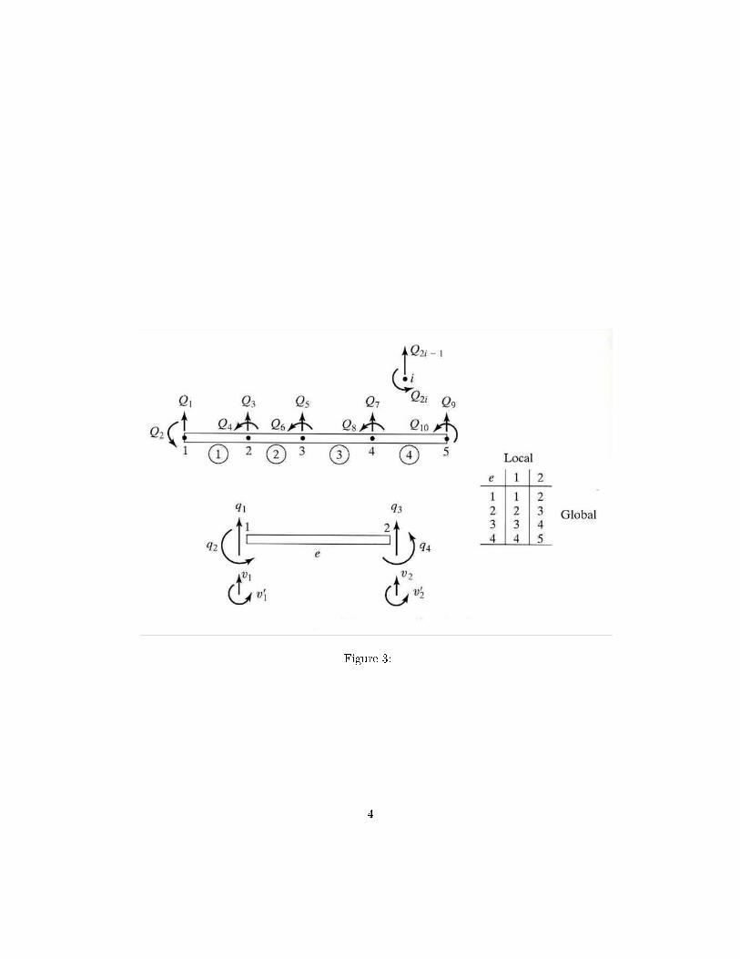
Figure 3:

4

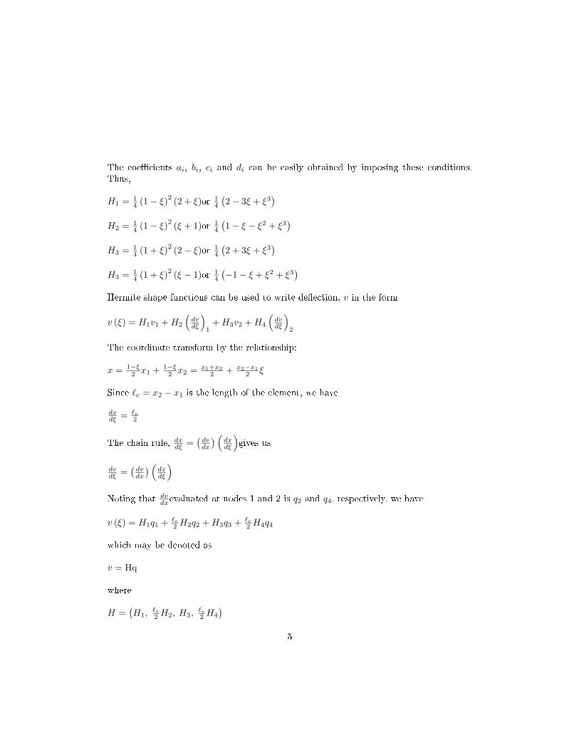
The coe�cients ai, bi, ci and di can be easily obtained by imposing these conditions.Thus,

H1 = 14 (1− ξ)2 (2 + ξ)or 1

4

(2− 3ξ + ξ3

)H2 = 1

4 (1− ξ)2 (ξ + 1)or 14

(1− ξ − ξ2 + ξ3

)H3 = 1

4 (1 + ξ)2 (2− ξ)or 14

(2 + 3ξ + ξ3

)H3 = 1

4 (1 + ξ)2 (ξ − 1)or 14

(−1− ξ + ξ2 + ξ3

)Hermite shape functions can be used to write de�ection, v in the form

v (ξ) = H1v1 +H2

(dvdξ

)1

+H3v2 +H4

(dvdξ

)2

The coordinate transform by the relationship:

x = 1−ξ2 x1 + 1−ξ

2 x2 = x1+x22 + x2−x1

2 ξ

Since `e = x2 − x1 is the length of the element, we have

dxdξ = `e

2

The chain rule, dxdξ =(dvdx

) (dxdξ

)gives us

dvdξ =

(dvdx

) (dxdξ

)Noting that dv

dxevaluated at nodes 1 and 2 is q2 and q4, respectively, we have

v (ξ) = H1q1 + `e2 H2q2 +H3q3 + `e

2 H4q4

which may be denoted as

v = Hq

where

H =(H1,

`e2 H2, H3,

`e2 H4

)5

Figure 4:

Element strain energy given by:

Ue = 12EI´e

(d2vdx2

)2

dx

Where the element sti�ness matrix is:

ke = EI`e

12 6`e −12 6`e6`e 4`2e −6`e 2`2e−12 −6`e 12 −6`e6`e 2`2e −6`e 4`2e

5.4 Load Vector

Referring to Figure 5.4 above, the equivalent load on an element, is given by:

fe =[p`e2 ,

p`2e12 ,

p`e2 ,−p`2e12

]T

6

5.5 Shear Force and Bending Moment

Using the bending moment and shear force equations,

M = EI d2vdx2 , V = dM

dx and v = Hq

we get the element bending moment and shear force:

M = EI`2e

[6ξq1 + (3ξ − 1) `eq2 − 6ξq3 + (3ξ + 1) `eq4]

V = 6EI`3e

[2q1 + `eq2 − 2q3 + `eq4]

Reaction force equation is given by: R = KQ− F

Example:

For the beam and loading in Figure 5.5 below, determine (1) the slope at 2 and 3 and (2)the vertical de�ection at the midpoint of the distributed load:

Solution:

We consider the two elements formed by the three nodes.Displacements Q1, Q2, Q3andQ5are constrained to be zero, and Q4and Q6need to be found. Since the lengths andsections are equal, the element sti�ness matrices are calculated as follows:

ke = EI`e

12 6`e −12 6`e6`e 4`2e −6`e 2`2e−12 −6`e 12 −6`e6`e 2`2e −6`e 4`2e

Element sti�ness matrices for element 1 and 2 are given by:

k1 = k2 = 8× 105

12 6 −12 66 4 −6 2−12 −6 12 −66 2 −6 4

e = 1 Q1 Q2 Q3 Q4

e = 2 Q3 Q4 Q5 Q6

7

Figure 5:

8

Refer to the Figure 5.4, the global applied loads are F4 = −1000 Nm and F4 = +1000 Nmobtained from

p`2e12 . We use here the elimination approach. Using the connectivity, we

obtain the global sti�ness matrix after elimination:

K =[k144 + k2

22 k224

k242 k2

44

]= 8× 105

[8 22 4

]

Because Q1, Q2, Q3and Q5are zero, the set of equation is given by:

8× 105

[8 22 4

]{Q4

Q6

}={−1000+1000

}

The solution is:

{Q4

Q6

}={−2.679× 10−4

4.464× 10−4

}

For element 2, q1 = 0, q2 = Q4, q3 = 0 and q4 = Q6 . To get vertical de�ection at themidpoint, use v = Hq at ξ = 0.

v = 0 + `e2 H2Q4 + 0 + `e

2 H4Q6

=(

12

) (14

) (−2.679× 10−4

)+(

12

) (− 1

4

) (4.464× 10−4

)= −8.93× 10−5 m

= −0.0893 mm

Problem above can be solved using BEAM program:

Input data for BEAM program:

9

B3JB2IB1

2000001

EMAT#

1.00E+066

-60005-1.00E+064

-60003

LOADDOF#

0503

02

01

Displ.DOF#4.00E+061322

4.00E+061211

Mom_InertiaMAT#N2N1EL#

2000310002

01

X-COORDNODE#

044

NMPCNLND

221123

NDNNENNDIMNMNENN

EXAMPLE 8.1

<< BEAM ANALYSIS >>

B3JB2IB1

2000001

EMAT#

1.00E+066

-60005-1.00E+064

-60003

LOADDOF#

0503

02

01

Displ.DOF#4.00E+061322

4.00E+061211

Mom_InertiaMAT#N2N1EL#

2000310002

01

X-COORDNODE#

044

NMPCNLND

221123

NDNNENNDIMNMNENN

EXAMPLE 8.1

<< BEAM ANALYSIS >>

Results from BEAM program:

5142.8665

8142.8023

-4285352

-1285.671

ReactionDOF#

0.00044643-1.6E-103

-0.00026786-2.5E-102

1.3392E-084.02E-111

RotationDispl.Node#

EXAMPLE 8.1

Results from Program BEAM

5142.8665

8142.8023

-4285352

-1285.671

ReactionDOF#

0.00044643-1.6E-103

-0.00026786-2.5E-102

1.3392E-084.02E-111

RotationDispl.Node#

EXAMPLE 8.1

Results from Program BEAM

5.6 Plane Frames

Here, we consider plane structures with rigidly connected members. These members willbe similar to the beams except that axial loads and axial deformations are present. The

10

Figure 6:

elements also have di�erent orientations. Figure 5.6 below shows a frame element. Foreach node, we have two displacements and a rotational deformation.

The nodal displacement vector in the global system is given by:

q = [q1, q2, q3, q4, q5, q6] T

The nodal displacement vector in the local system is given by:

q′ = [q′1, q′2, q

′3, q

′4, q

′5, q

′6]

T

Local-global transformation is:

q′ = Lq1

where :

L =

` m 0 0 0 0−m ` 0 0 0 00 0 1 0 0 00 0 0 ` m 00 0 0 −m ` 00 0 0 0 0 1

11

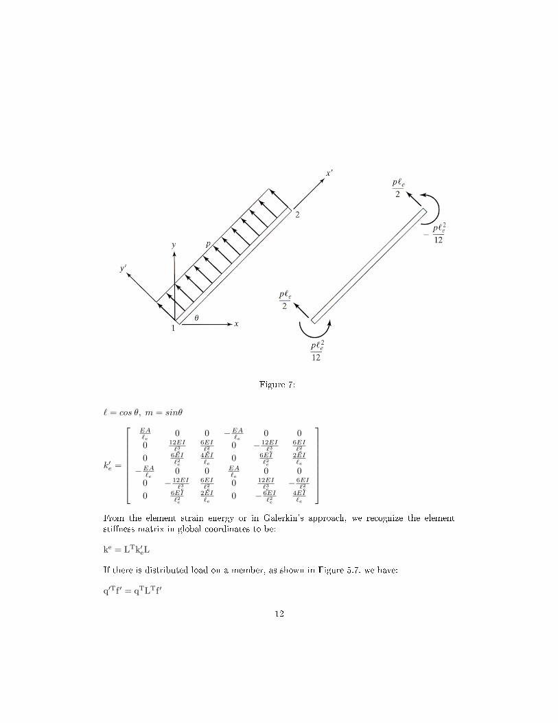
Figure 7:

` = cos θ, m = sinθ

k′e =

EA`e

0 0 −EA`e 0 00 12EI

`3e

6EI`2e

0 − 12EI`3e

6EI`2e

0 6EI`2e

4EI`e

0 6EI`2e

2EI`e

−EA`e 0 0 EA`e

0 00 − 12EI

`3e

6EI`2e

0 12EI`3e

− 6EI`2e

0 6EI`2e

2EI`e

0 − 6EI`2e

4EI`e

From the element strain energy or in Galerkin's approach, we recognize the elementsti�ness matrix in global coordinates to be:

ke = LTk′eL

If there is distributed load on a member, as shown in Figure 5.7, we have:

q′Tf ′ = qTLTf ′

12

where f ′ =[0, p`e2 ,

p`2e12 , 0, p`e2 , −p`

2e

12

]T

The nodal loads due to the distributed load, p are given by:

f = LTf ′

The system of equations:

KQ = F

where penalty approach is applied to solve the equations.

Example:

Detremine the displacements and rotations of the joints for the portal frame shown inFigure 5.8 below.

Solution:

The connectivity is as follows:

Element No. Node1 2

1 1 22 3 13 4 2

Element Sti�ness

Element 1: Noting that, k1 = k′1, we �nd that

Q1 Q2 Q3 Q4 Q5 Q6

k1 = 104×

141.7 0 0 −141.7 0 0

0 0.784 56.4 0 −0.784 56.40 56.4 5417 0 −56.4 2708

−141.7 0 0 141.7 0 00 −0.784 −56.4 0 0.784 −56.40 56.4 2708 0 −56.4 5417

Q1

Q2

Q3

Q4

Q5

Q6

Elements 2 and 3:

13

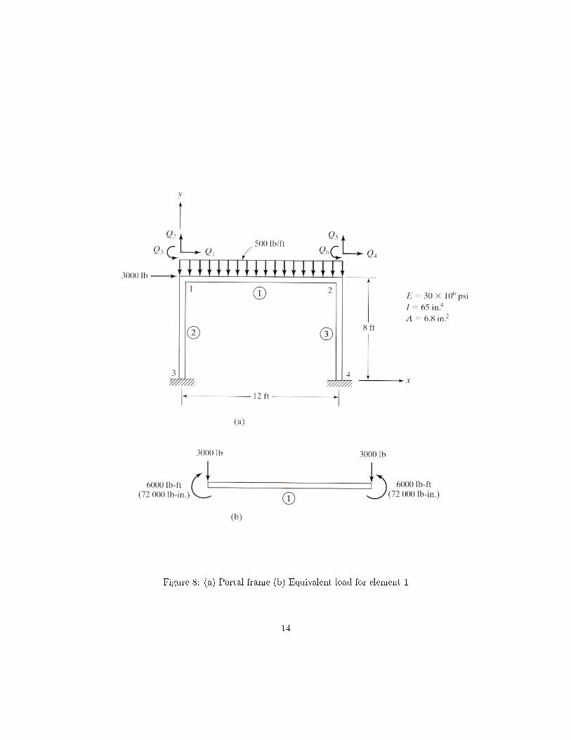
Figure 8: (a) Portal frame (b) Equivalent load for element 1

14

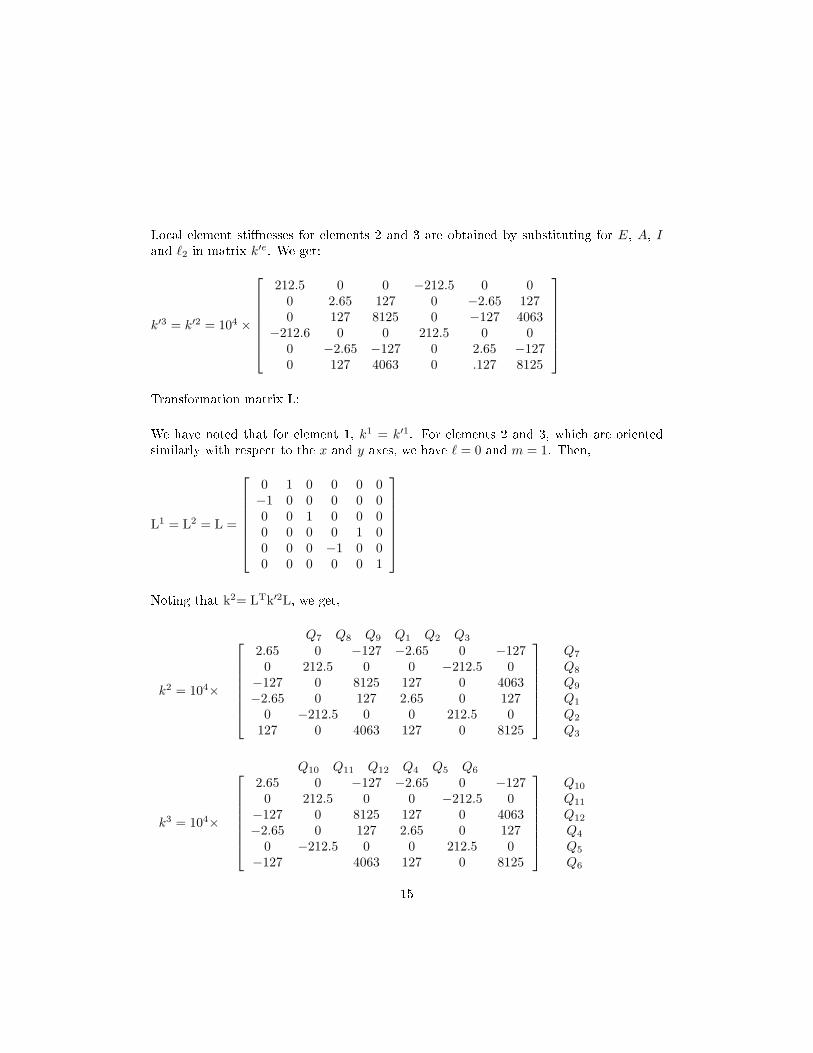
Local element sti�nesses for elements 2 and 3 are obtained by substituting for E, A, Iand `2 in matrix k′e. We get:

k′3 = k′2 = 104 ×

212.5 0 0 −212.5 0 0

0 2.65 127 0 −2.65 1270 127 8125 0 −127 4063

−212.6 0 0 212.5 0 00 −2.65 −127 0 2.65 −1270 127 4063 0 .127 8125

Transformation matrix L:

We have noted that for element 1, k1 = k′1. For elements 2 and 3, which are orientedsimilarly with respect to the x and y axes, we have ` = 0 and m = 1. Then,

L1 = L2 = L =

0 1 0 0 0 0−1 0 0 0 0 00 0 1 0 0 00 0 0 0 1 00 0 0 −1 0 00 0 0 0 0 1

Noting that k2= LTk′2L, we get,

Q7 Q8 Q9 Q1 Q2 Q3

k2 = 104×

2.65 0 −127 −2.65 0 −1270 212.5 0 0 −212.5 0−127 0 8125 127 0 4063−2.65 0 127 2.65 0 127

0 −212.5 0 0 212.5 0127 0 4063 127 0 8125

Q7

Q8

Q9

Q1

Q2

Q3

Q10 Q11 Q12 Q4 Q5 Q6

k3 = 104×

2.65 0 −127 −2.65 0 −1270 212.5 0 0 −212.5 0−127 0 8125 127 0 4063−2.65 0 127 2.65 0 127

0 −212.5 0 0 212.5 0−127 4063 127 0 8125

Q10

Q11

Q12

Q4

Q5

Q6

15

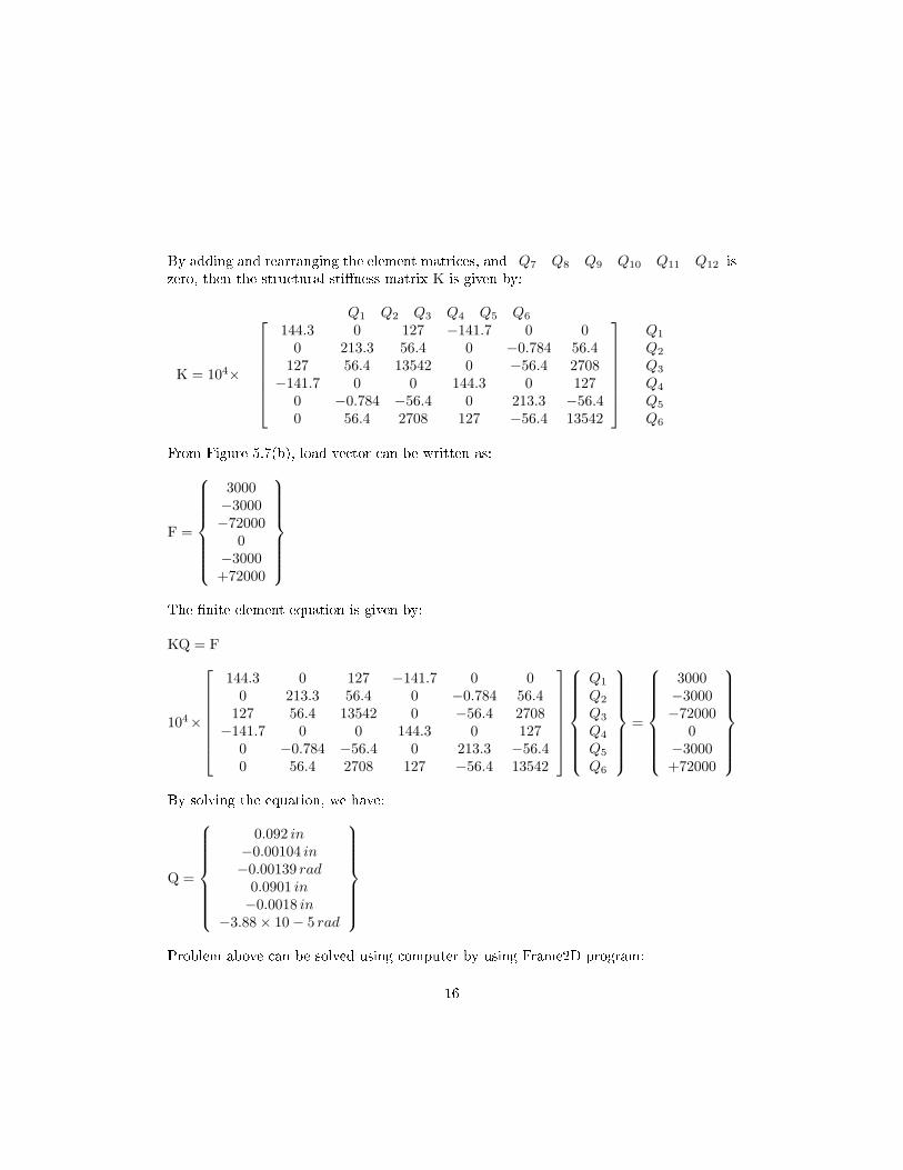
By adding and rearranging the element matrices, and Q7 Q8 Q9 Q10 Q11 Q12 iszero, then the structural sti�ness matrix K is given by:

Q1 Q2 Q3 Q4 Q5 Q6

K = 104×

144.3 0 127 −141.7 0 0

0 213.3 56.4 0 −0.784 56.4127 56.4 13542 0 −56.4 2708−141.7 0 0 144.3 0 127

0 −0.784 −56.4 0 213.3 −56.40 56.4 2708 127 −56.4 13542

Q1

Q2

Q3

Q4

Q5

Q6

From Figure 5.7(b), load vector can be written as:

F =

3000−3000−72000

0−3000+72000

The �nite element equation is given by:

KQ = F

104×

144.3 0 127 −141.7 0 0

0 213.3 56.4 0 −0.784 56.4127 56.4 13542 0 −56.4 2708−141.7 0 0 144.3 0 127

0 −0.784 −56.4 0 213.3 −56.40 56.4 2708 127 −56.4 13542

Q1

Q2

Q3

Q4

Q5

Q6

=

3000−3000−72000

0−3000+72000

By solving the equation, we have:

Q =

0.092 in−0.00104 in−0.00139 rad

0.0901 in−0.0018 in

−3.88× 10− 5 rad

Problem above can be solved using computer by using Frame2D program:

16

(Multi-point constr.B1*Qi+B2*Qj=B3)B3jB2iB1

3.00E+071

EMAT#30001

LoadDOF#012

011010

090807

Displ.DOF#0656.812430656.81132

41.6666656.81121Distr_LoadInertiaAreaMat#N2N1Elem#

01444

003961442

9601YXNode#

016NMPCNLND

322134NDNNENNDIMNMNENN

EXAMPLE 8.2<<2-D FRAME ANALYSIS >>

(Multi-point constr.B1*Qi+B2*Qj=B3)B3jB2iB1

3.00E+071

EMAT#30001

LoadDOF#012

011010

090807

Displ.DOF#0656.812430656.81132

41.6666656.81121Distr_LoadInertiaAreaMat#N2N1Elem#

01444

003961442

9601YXNode#

016NMPCNLND

322134NDNNENNDIMNMNENN

EXAMPLE 8.2<<2-D FRAME ANALYSIS >>

Figure 9:

Input data for Frame2D program:

Result from Frame2D program:

5.7 Three-dimensional Frames

Three dimensional frames, also called as space frames, are frequently encountered in theanalysis of multistory buidings. They are also to be found in the modeling of car bodyand bicycle frames. A typical three-dimensional frame is shown in Figure 5.8 below. Eachnode has six degree of freedom (as opposed to only three dofs in a plane frame).

Local coordinate system is given by:

q′ =[q′1, q

′2, q′3︸ ︷︷ ︸ , q′4, q

′5, q′6︸ ︷︷ ︸ , q′7, q

′8, q′9︸ ︷︷ ︸ , q′10, q

′11, q

′12︸ ︷︷ ︸]

Translasi nod 1 Putaran nod 1 Translasi nod 2 Putaran nod 2

Global coordinate system is given by:

17

112828.8123798.83111-2334.210

60138.8192201.1598

-665.87ReactionDOF#

111254.4-2334.2-3798.83112828.82334.23798.831

3Member#3777.949-665.8-2201.1660138.81665.79962201.159

2Member#-75777.8798.836-2334.2-39254.6-798.8362334.2

1Member#Member End-Forces

-8.3E-08-2.8E-091.72E-094-4.4E-08-1.6E-094.92E-103-3.9E-05-0.001790.0901222-0.00139-0.001040.091771

Z-RotationY-DisplX-DisplNode#EXAMPLE 8.2Results from Program Frame2D

112828.8123798.83111-2334.210

60138.8192201.1598

-665.87ReactionDOF#

111254.4-2334.2-3798.83112828.82334.23798.831

3Member#3777.949-665.8-2201.1660138.81665.79962201.159

2Member#-75777.8798.836-2334.2-39254.6-798.8362334.2

1Member#Member End-Forces

-8.3E-08-2.8E-091.72E-094-4.4E-08-1.6E-094.92E-103-3.9E-05-0.001790.0901222-0.00139-0.001040.091771

Z-RotationY-DisplX-DisplNode#EXAMPLE 8.2Results from Program Frame2D

Figure 10:

Figure 11:

18

Figure 12:

q =[q′1, q

′2, q′3, q′4, q′5, q′6, q′7, q′8, q′9, q′10, q

′11, q

′12︸ ︷︷ ︸

V ektor anjakan dalamsistemsejagat x,y dan z

]

Local coordinate system is established with the use of three points. Points 1 and 2 arethe ends of the element; the x′-axis is along the line from point 1 to point 2, just in thecase of two-dimensional frames. Point 3 is any reference point not laying along the linejoining points 1 and 2. The y′-axis is to lie in the plane de�ned by points 1, 2 and 3.The z′-axis is then automatically de�ned from the fact that x′, y′and z′ form a righthanded system. We note that y′, z′are the principal axes of the cross section with Iy′ andIz′ are the principal moments of inertia. The cross-sectional properties are speci�ed byfour parameters: area A, and moments of inertia Iy′, Iz′, and J . The product GJ is thetorsional sti�ness, where G = shear modulus. For circular or tubular cross section, J isthe polar moment of inertia. For other cross-sectional shapes, such as an I-section, thetorsional sti�ness is given in the strength of materials texts.

The (12x12) element sti�ness matrix, in the local coordinate system is given by:

19

k′ =

AS 0 0 0 0 0 −AS 0 0 0 0 0a

′

z 0 0 0 b′

z 0 −a′z 0 0 0 b′za′y 0 −by 0 0 0 −a′y 0 b′y 0

TS 0 0 0 0 0 −TS 0 0c′y 0 0 0 b′y 0 d′y 0

c′z 0 −b′z 0 0 0 d′zAS 0 0 0 0 0

a′z 0 0 0 −b′zc′y 0 b′y 0

TS 0 0c′y 0

symmetry c′z

where:

AS = EAle, le = element length, TS = GJ

le, a′z = 12EIz′

l3e, b′z = 6EI

l3e

c′

z =4EI

z′

le, d

′

z =2EI

z′

l′e,a

′

y =12EI

y′

l3eand so on.

The global-local transformation matrix is given by:

q = Lq

The (12x12) transformation matrix L is de�ned as:

L =

l1 m1 n1 0 0 0 0 0 0 0 0 0l2 m2 n2 0 0 0 0 0 0 0 0 0l3 m3 n3 0 0 0 0 0 0 0 0 00 0 0 l1 m1 n1 0 0 0 0 0 00 0 0 l2 m2 n2 0 0 0 0 0 00 0 0 l3 m3 n3 0 0 0 0 0 00 0 0 0 0 0 l1 m1 n1 0 0 00 0 0 0 0 0 l2 m2 n2 0 0 00 0 0 0 0 0 l3 m3 n3 0 0 00 0 0 0 0 0 0 0 0 l1 m1 n1

0 0 0 0 0 0 0 0 0 l2 m2 n2

0 0 0 0 0 0 0 0 0 l3 m3 n3

or

20

L =

λ 0

λλ

0 λ

where

λ =

l1 m1 n1

l2 m2 n2

l3 m3 n3

l1, m1and n1are the cosines of the angles between the x′-axis and the global x, y and zaxes. Similarly l2, m2and n2 are the cosines of the angles between the y′-axis and theglobal x, y and z axes. and are the cosines of the angles between the axes and the globalx, y and z axes.

These direction cosines and hence the λ matrix are obtainable from the coordinates ofthe points 1, 2 and 3 as follows:

l1 = x2−x1le

with le =√

(x2 − x1)2 + (y2 − y1)2 + (z2 − z1)2

m1 = y2−y1le

n1 = z2−z1le

The element sti�ness matrix in global coordinates is:

k = LTk′L

If a distributed load with components w′y and w′z (units of force/unit length) is appliedon the element, then the equivalent loads at the ends of the member are:

f ′ =[0, wy′ le

2 , wz′ le2 , 0, −wz′ l2e

12 ,wy′ l2e

12 , 0, wy′ le2 , wz′ le

2 , 0, −wz′ l2e12 ,

wy′ l2e12

]T

These loads are transferred into global components by f = LTf ′. After enforcing boundaryconditions and solving the system equations KQ = F, we can compute the member endforces from

R′ = k′q′ + fixed end reactions

21

Figure 13:

where the �xed-end reactions are the negative of the f ′ vector and are only associatedwith those elements having distributed loads acting on them.

Example

Figure 5.10 shows a three-dimensional frame subjected to various loads. By runningFrame3D program, �nd the maximum bending moments in the structure.

Input data for Frame3D program:

22

8.00E+102.00E+111GEMAT#

-18000024-600002024000015

LoadDOF#

030029028027026

025060504

030201

Displ.DOF#000.0020.0010.0010.0116544000.0020.0010.0010.0116433000.0020.0010.0010.01163220-400000.0020.0010.0010.0117211

UDLz'UDLy'JIzIyAreaMat#Ref_PtN2N1Elem#00-370666

30950364033303020001

ZYXNode#0312

NMPCNLND

2623145NNREFNDNNENNDIMNMNENN

EXAMPLE <<3- D Frame Analysis >>

8.00E+102.00E+111GEMAT#

-18000024-600002024000015

LoadDOF#

030029028027026

025060504

030201

Displ.DOF#000.0020.0010.0010.0116544000.0020.0010.0010.0116433000.0020.0010.0010.01163220-400000.0020.0010.0010.0117211

UDLz'UDLy'JIzIyAreaMat#Ref_PtN2N1Elem#00-370666

30950364033303020001

ZYXNode#0312

NMPCNLND

2623145NNREFNDNNENNDIMNMNENN

EXAMPLE <<3- D Frame Analysis >>

Result from Frame3D program:

1.47E+0430-1.12E+0529-9.31E+0428-1.08E+05278.63E+0426-7.83E+0425-7.13E+0469.53E+045-3.68E+054-1.32E+053-2.63E+042-4.17E+041ReactionDOF#

7.62E+04-1.24E+051.96E+04-2.10E+04-5.60E+03-1.57E+05

-4.71E+041.47E+04-1.96E+042.10E+045.60E+031.57E+05End Forces4Member#

-1.41E+05-2.33E+04-2.80E+04-1.08E+052.63E+04-7.83E+04

6.25E+04-3.01E+052.80E+041.08E+05-2.63E+047.83E+04End Forces3Member#

-6.25E+043.01E+05-2.80E+041.32E+052.63E+04-7.83E+04-1.64E+049.53E+042.80E+04-1.32E+05-2.63E+047.83E+04

End Forces2Member#

4.64E+042.80E+04-9.53E+041.32E+051.83E+042.63E+04-1.01E+053.68E+059.53E+04-1.32E+05-1.83E+04-2.63E+04

End Forces1Member#Member End-Forces

-1.10E-098.43E-096.98E-098.10E-09-6.47E-095.87E-095-7.66E-041.84E-031.50E-036.24E-033.43E-03-2.10E-0347.62E-04-2.45E-042.03E-039.84E-033.14E-03-1.99E-0331.11E-03-1.79E-032.55E-035.31E-033.94E-05-1.87E-0325.35E-09-7.14E-092.76E-089.90E-091.97E-093.13E-091Z-RotY-RotX-RotZ-DisplY-DisplX-DisplNode#

EXAMPLE Results from Program Frame3D

1.47E+0430-1.12E+0529-9.31E+0428-1.08E+05278.63E+0426-7.83E+0425-7.13E+0469.53E+045-3.68E+054-1.32E+053-2.63E+042-4.17E+041ReactionDOF#

7.62E+04-1.24E+051.96E+04-2.10E+04-5.60E+03-1.57E+05

-4.71E+041.47E+04-1.96E+042.10E+045.60E+031.57E+05End Forces4Member#

-1.41E+05-2.33E+04-2.80E+04-1.08E+052.63E+04-7.83E+04

6.25E+04-3.01E+052.80E+041.08E+05-2.63E+047.83E+04End Forces3Member#

-6.25E+043.01E+05-2.80E+041.32E+052.63E+04-7.83E+04-1.64E+049.53E+042.80E+04-1.32E+05-2.63E+047.83E+04

End Forces2Member#

4.64E+042.80E+04-9.53E+041.32E+051.83E+042.63E+04-1.01E+053.68E+059.53E+04-1.32E+05-1.83E+04-2.63E+04

End Forces1Member#Member End-Forces

-1.10E-098.43E-096.98E-098.10E-09-6.47E-095.87E-095-7.66E-041.84E-031.50E-036.24E-033.43E-03-2.10E-0347.62E-04-2.45E-042.03E-039.84E-033.14E-03-1.99E-0331.11E-03-1.79E-032.55E-035.31E-033.94E-05-1.87E-0325.35E-09-7.14E-092.76E-089.90E-091.97E-093.13E-091Z-RotY-RotX-RotZ-DisplY-DisplX-DisplNode#

EXAMPLE Results from Program Frame3D

5.8 Case Study/Engineering Application:

ANALYSIS OF THE STABILIZER BAR UNDER LOADING CONDITION

23

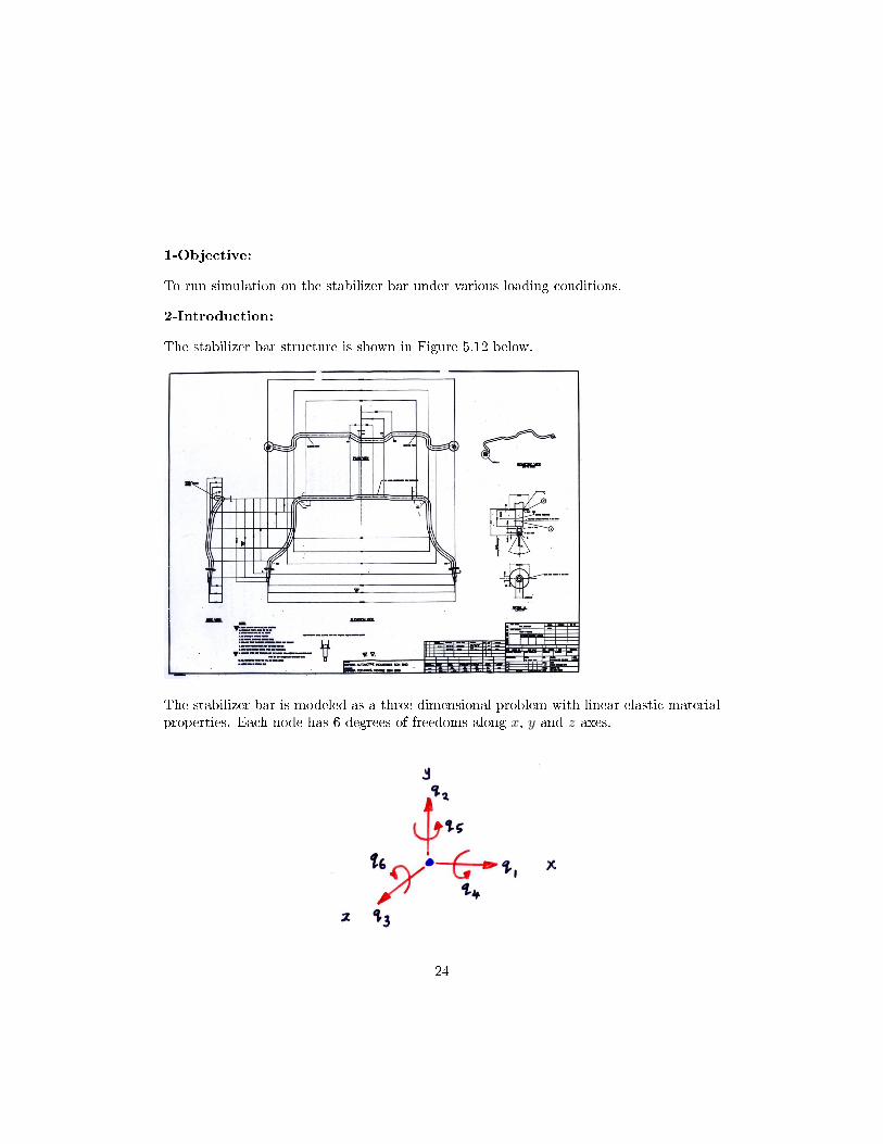
1-Objective:

To run simulation on the stabilizer bar under various loading conditions.

2-Introduction:

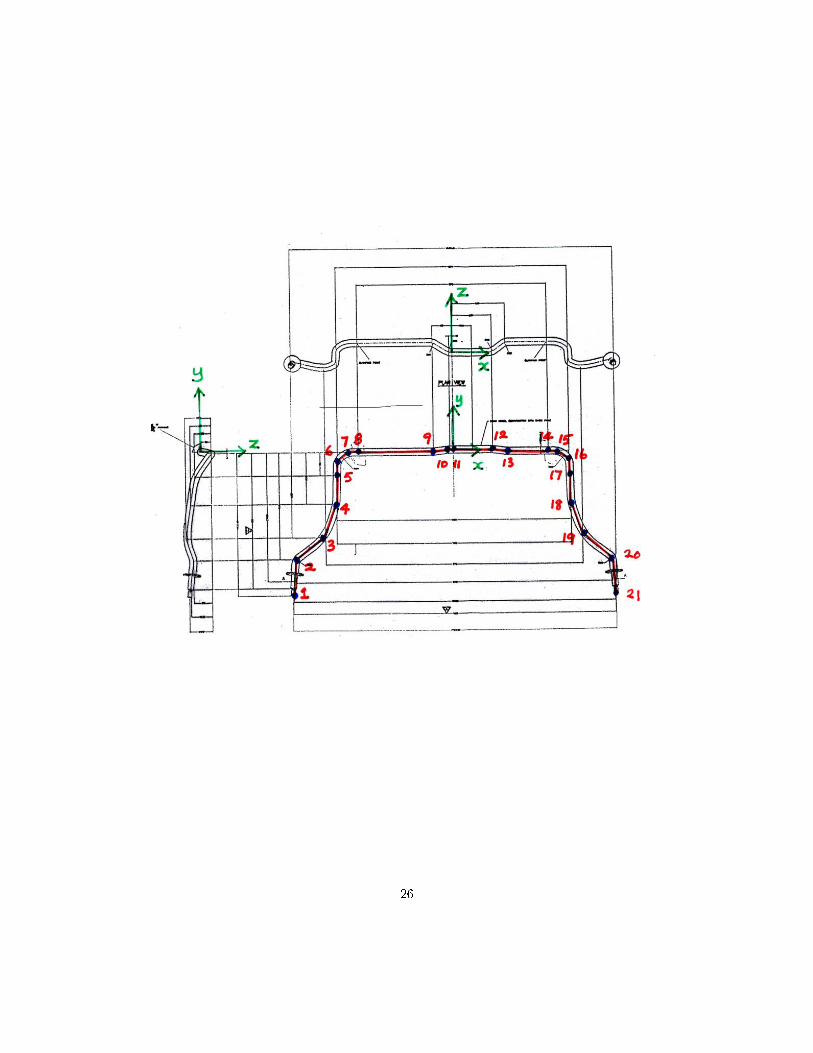
The stabilizer bar structure is shown in Figure 5.12 below.

The stabilizer bar is modeled as a three dimensional problem with linear elastic materialproperties. Each node has 6 degrees of freedoms along x, y and z axes.

24

q = [q1, q2, q3, q4, q5, q6] T

The local sti�ness matrix, k (12 x 12 matrix) is a function of element sti�ness (EA/l),torsional sti�ness (GJ/l)and moment of inertia I. Global sti�ness matrix is:

K = LTkL

where L is the local-global transformation matrix. After applying boundary conditions,the system equation is given by:

KQ = F

where Qis the displacement and F is load.

3-Element Geometry:

25

26

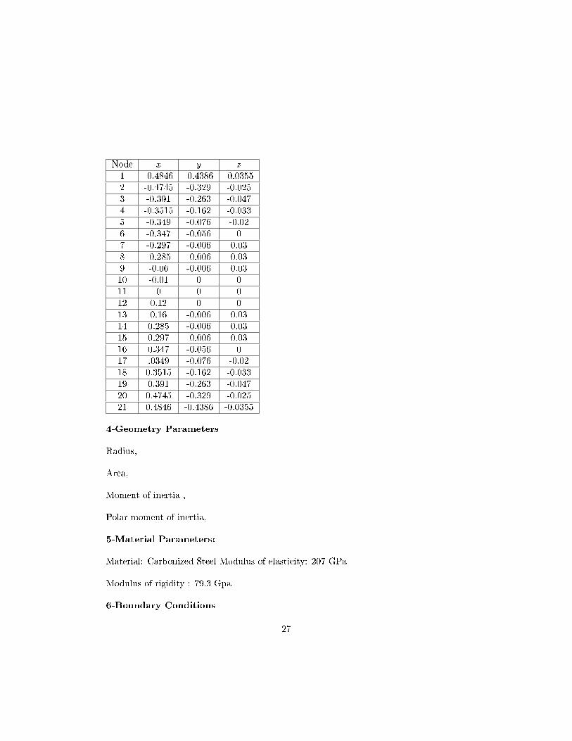
Node x y z

1 -0.4846 -0.4386 -0.03552 -0.4745 -0.329 -0.0253 -0.391 -0.263 -0.0474 -0.3515 -0.162 -0.0335 -0.349 -0.076 -0.026 -0.347 -0.056 07 -0.297 -0.006 0.038 -0.285 -0.006 0.039 -0.06 -0.006 0.0310 -0.01 0 011 0 0 012 0.12 0 013 0.16 -0.006 0.0314 0.285 -0.006 0.0315 0.297 -0.006 0.0316 0.347 -0.056 017 .0349 -0.076 -0.0218 0.3515 -0.162 -0.03319 0.391 -0.263 -0.04720 0.4745 -0.329 -0.02521 0.4846 -0.4386 -0.0355

4-Geometry Parameters

Radius,

Area,

Moment of inertia ,

Polar moment of inertia,

5-Material Parameters:

Material: Carbonized Steel Modulus of elasticity: 207 GPa

Modulus of rigidity : 79.3 Gpa

6-Boundary Conditions

27

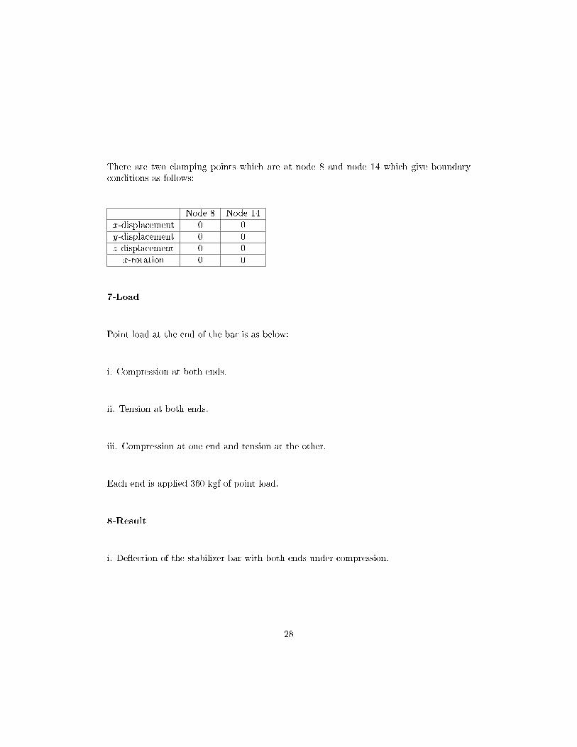
There are two clamping points which are at node 8 and node 14 which give boundaryconditions as follows:

Node 8 Node 14x -displacement 0 0y-displacement 0 0z -displacement 0 0

x -rotation 0 0

7-Load

Point load at the end of the bar is as below:

i. Compression at both ends.

ii. Tension at both ends.

iii. Compression at one end and tension at the other.

Each end is applied 360 kgf of point load.

8-Result

i. De�ection of the stabilizer bar with both ends under compression.

28

Node x -de�ection y-de�ection z -de�ection1 -115.28 52.412 -7.211 -0.15 -23.97 -1.321 116.257 52.861 -7.2

ii. De�ection of the stabilizer bar with both ends under tension.

29

Node x -de�ection y-de�ection z -de�ection1 115.2 -52.41 7.19511 0.1519 23.97 1.30421 -116.2 -52.86 7.195

iii. De�ection of the stabilizer bar with compression at one end and tension at the otherend.

30

Node x -de�ection y-de�ection z -de�ection1 67.145 -30.20 7.19511 0.107 -0.12 -0.2421 68.12 30.65 -7.184

9- Appendix Input data for Frame3D program for cases where both ends are

under compression.

31

(Multi-point constr. B1*Qi+B2*Qj=B3)

B3jB2iB1

7.93E+102.07E+111

GEMAT#

3531.6122

3531.62

LoadDOF#

083

082

081

080

079

047

046

045

044

043

Displ.DOF#

001.2005E-086.0026E-096.0026E-092.7465E-04124212020

001.2005E-086.0026E-096.0026E-092.7465E-04124201919

001.2005E-086.0026E-096.0026E-092.7465E-04124191818

001.2005E-086.0026E-096.0026E-092.7465E-04124181717

001.2005E-086.0026E-096.0026E-092.7465E-04124171616

001.2005E-086.0026E-096.0026E-092.7465E-04123161515

001.2005E-086.0026E-096.0026E-092.7465E-04123151414

001.2005E-086.0026E-096.0026E-092.7465E-04123141313

001.2005E-086.0026E-096.0026E-092.7465E-04123131212

001.2005E-086.0026E-096.0026E-092.7465E-04123121111

001.2005E-086.0026E-096.0026E-092.7465E-04123111010

001.2005E-086.0026E-096.0026E-092.7465E-041231099

001.2005E-086.0026E-096.0026E-092.7465E-04123988

001.2005E-086.0026E-096.0026E-092.7465E-04123877

001.2005E-086.0026E-096.0026E-092.7465E-04123766

001.2005E-086.0026E-096.0026E-092.7465E-04122655

001.2005E-086.0026E-096.0026E-092.7465E-04122544

001.2005E-086.0026E-096.0026E-092.7465E-04122433

001.2005E-086.0026E-096.0026E-092.7465E-04122322

001.2005E-086.0026E-096.0026E-092.7465E-04122211

UDLz'UDLy'JIzIyAreaMat#Ref_PtN2N1Elem#

0.03-0.0060.34724

010023

0.03-0.006-0.34722

-0.0355-0.43860.484621

-0.025-0.3290.474520

-0.047-0.2630.39119

-0.033-0.1620.351518

-0.02-0.0760.34917

0-0.0560.34716

0.03-0.0060.29715

0.03-0.0060.28514

0.03-0.0060.1613

000.1212

00011

00-0.0110

0.03-0.006-0.069

0.03-0.006-0.2858

0.03-0.006-0.2977

0-0.056-0.3476

-0.02-0.076-0.3495

-0.033-0.162-0.35154

-0.047-0.263-0.3913

-0.025-0.329-0.47452

-0.0355-0.4386-0.48461

ZYXNode#

0210

NMPCNLND

362312021

NNREFNDNNENNDIMNMNENN

Stabilizer Bar Deflection Analysis

<<3-D Frame Analysis >>

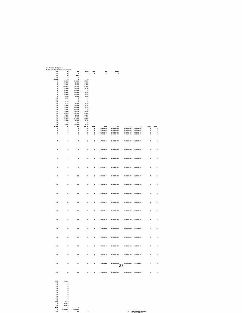
(Multi-point constr. B1*Qi+B2*Qj=B3)

B3jB2iB1

7.93E+102.07E+111

GEMAT#

3531.6122

3531.62

LoadDOF#

083

082

081

080

079

047

046

045

044

043

Displ.DOF#

001.2005E-086.0026E-096.0026E-092.7465E-04124212020

001.2005E-086.0026E-096.0026E-092.7465E-04124201919

001.2005E-086.0026E-096.0026E-092.7465E-04124191818

001.2005E-086.0026E-096.0026E-092.7465E-04124181717

001.2005E-086.0026E-096.0026E-092.7465E-04124171616

001.2005E-086.0026E-096.0026E-092.7465E-04123161515

001.2005E-086.0026E-096.0026E-092.7465E-04123151414

001.2005E-086.0026E-096.0026E-092.7465E-04123141313

001.2005E-086.0026E-096.0026E-092.7465E-04123131212

001.2005E-086.0026E-096.0026E-092.7465E-04123121111

001.2005E-086.0026E-096.0026E-092.7465E-04123111010

001.2005E-086.0026E-096.0026E-092.7465E-041231099

001.2005E-086.0026E-096.0026E-092.7465E-04123988

001.2005E-086.0026E-096.0026E-092.7465E-04123877

001.2005E-086.0026E-096.0026E-092.7465E-04123766

001.2005E-086.0026E-096.0026E-092.7465E-04122655

001.2005E-086.0026E-096.0026E-092.7465E-04122544

001.2005E-086.0026E-096.0026E-092.7465E-04122433

001.2005E-086.0026E-096.0026E-092.7465E-04122322

001.2005E-086.0026E-096.0026E-092.7465E-04122211

UDLz'UDLy'JIzIyAreaMat#Ref_PtN2N1Elem#

0.03-0.0060.34724

010023

0.03-0.006-0.34722

-0.0355-0.43860.484621

-0.025-0.3290.474520

-0.047-0.2630.39119

-0.033-0.1620.351518

-0.02-0.0760.34917

0-0.0560.34716

0.03-0.0060.29715

0.03-0.0060.28514

0.03-0.0060.1613

000.1212

00011

00-0.0110

0.03-0.006-0.069

0.03-0.006-0.2858

0.03-0.006-0.2977

0-0.056-0.3476

-0.02-0.076-0.3495

-0.033-0.162-0.35154

-0.047-0.263-0.3913

-0.025-0.329-0.47452

-0.0355-0.4386-0.48461

ZYXNode#

0210

NMPCNLND

362312021

NNREFNDNNENNDIMNMNENN

Stabilizer Bar Deflection Analysis

<<3-D Frame Analysis >>

32

For the case where both ends are under tension, the load on the degree of freedom 2 and122 becomes -3531.6 and -3531.6, while for the case where one end are under tension andthe other are under compression, the load becomes -3531.5 and 3531.6.

33