Ordinary di⁄erential equations and mathematical modelling ...

Chapter 5
Methods for ordinarydifferential equations
5.1 Initial-value problems
Initial-value problems (IVP) are those for which the solution is entirely knownat some time, say t = 0, and the question is to solve the ODE
y′(t) = f(t, y(t)), y(0) = y0,
for other times, say t > 0. We will consider a scalar y, but consideringsystems of ODE is a straightforward extension for what we do in this chapter.We’ll treat both theoretical questions of existence and uniqueness, as well aspractical questions concerning numerical solvers.
We speak of t as being time, because that’s usually the physical contextin which IVP arise, but it could very well be a space variable.
Does a solution exist, is it unique, and does it tend to infinity (blow up)in finite time? These questions are not merely pedantic. As we now showwith two examples, things can go wrong very quickly if we posit the wrongODE.
Example 12. Consider
y′ =√y, y(0) = 0.
By separation of variables, we find∫dy√ =y
∫(t+ C)2
dt ⇒ y(t) = .4
1

CHAPTER 5. METHODS FOR ORDINARY DIFFERENTIAL EQUATIONS
Imposing the initial condition yields C = 0, hence y(t) = t2/4. However,y(t) = 0 is clearly another solution, so we have non-uniqueness. In fact, thereis an infinite number of solutions, corresponding to y(t) = 0 for 0 ≤ t ≤ t∗ forsome t∗, which then takes off along the parabola the parabola y(t) = (t−t∗)2/4for times t ≥ t∗.
Example 13. Consider
y′ = y2, y(0) = 1.
By separation of variables, we find∫dy
=y2
∫dt ⇒ y(t) =
−1.
t+ C
The initial condition gives C = −1, hence y(t) = 1/(1 − t). It blows up attime t = 1, because y(t) has a vertical asymptote. We say that the solutionexists locally in any interval to the left of t = 1, but we don’t have globalexistence.
Blowup and non-uniqueness are generally, although not always1, unreal-istic in applications. A theory of existence and uniqueness, including globalexistence (non blowup), is desired to guide us in formulating valid modelsfor physical phenomena.
The basic result is the following.
Theorem 8. (Picard) For given T,C, and y0, consider the box B in (t, y)space, given by
B = [0, T ]× [y0 − C, y0 + C].
Assume that
• f(t, y) is continuous over B;
• |f(t, y)| ≤ K when (t, y) ∈ B; (boundedness)
• |f(t, u) − f(t, v)| ≤ L|u − v| when (t, u), (t, v) ∈ B. (Lipschitzcontinuity).
1In nonlinear optics for instance, laser pulses may “collapse”. This situation is some-what realistically modeled by an ODE that blows up, although not for times arbitrarilyclose to the singularity.
2
5.2. NUMERICAL METHODS FOR INITIAL-VALUE PROBLEMS
Assume furthermore that C ≥ K (eLT − 1). Then there exists a unique yL
∈C1[0, T ], such that
y′(t) = f(t, y(t)), y(0) = y0,
and such that |y(t) − y0| ≤ C. In short, the solution exists, is unique, andstays in the box for times 0 ≤ t ≤ T .
Proof. The technique is called Picard’s iteration. See p.311 in Suli-Mayers.
The ODE y′ =√y does not satisfy the assumptions of the theorem above
because the square root is not a Lipschitz function. The ODE y′ = y2 doesnot satisfy the assumptions of the theorem above because y2 is not boundedby a constant K.
5.2 Numerical methods for Initial-Value Prob-
lems
Here is an overview of some of the most popular numerical methods forsolving ODEs. Let tn = nh, and denote by yn the approximation of y(tn).
1. Forward Euler (a.k.a. explicit Euler).
yn+1 = yn + hf(tn, yn).
This formula comes from approximating the derivative y′ at t = tn bya forward difference. It allows to march in time from the knowledge ofyn, to get yn+1.
2. Backward Euler (a.k.a. implicit Euler).
yn+1 = yn + hf(tn+1, yn+1).
This time we use a backward difference for approximating the derivativeat t = tn+1. The unknown yn+1 appears implicitly in this equation,hence the name implicit. It still needs to be solved for as a functionof yn, using (for instance) Newton’s method. The strategy is still tomarch in time, but at every step there is a nonlinear equation to solve.
3

CHAPTER 5. METHODS FOR ORDINARY DIFFERENTIAL EQUATIONS
3. Trapezoidal (a.k.a. midpoint) rule (implicit).
hyn+1 = yn + [f(tn, yn) + f(tn+1, yn+1)] .
2
In this equation yn+1−yn has the interpretation of a centered differenceh
about the midpoint tn+ 1 = tn+tn+1 , but since f(tn+ 1 , yn+ 1 ) is not ac-2 2 2 2
cessible (yn+ 1 is not part of what we wish to solve for), we replace it2
by the average 1 [f(tn, yn) + f(tn+1, yn+1)]. This gives a more balanced2
estimate of the slope yn+1−yn . It is an implicit method: yn+1 needs toh
be solved for.
4. Improved Euler, Runge-Kutta 2 (explicit).
yn+1 = yn + hf(tn, yn),
hyn+1 = yn + [f(tn, yn) + f(tn+1, yn+1)] .
2
This is the simplest of “predictor-corrector” methods. It is like themidpoint rule, except that we use a guess yn+1 for the unknown valueof yn+1 in the right-hand side, and this guess comes from the explicitEuler method. Now yn+1 only appears in the left-hand side, so this isan explicit method.
5. Runge-Kutta 4 (explicit).
yn+1 = yn + h[k1 + 2k2 + 2k3 + k4],
where the slopes k1, . . . , k4 are given in succession by
h hk1 = f(tn, yn), k2 = f(tn + , yn + k1),
2 2
h hk3 = f(tn + , yn + k2), k4 = f(tn + h, yn + hk3).
2 2
6. There are also methods that involve not just the past value yn, but alarger chunk of history yn−1, yn−2,etc. These methods are called multi-step. They are in general less flexible than the one-step methods de-scribed so far, in that they require a constant step h as we march intime.
4

5.2. NUMERICAL METHODS FOR INITIAL-VALUE PROBLEMS
Two features of a numerical method are important when choosing a nu-merical method:
• Is it convergent, i.e., does the computed solution tend to the true solu-tion as h→ 0, and at which rate?
• Is it stable, i.e., if we solve with different initial conditions y0 and y0,are the computed solutions close in the sense that |yn− yn| ≤ C|y0− y0|,with n = O(1/h), and C independent of h?
5.2.1 Convergence
To understand convergence better in the case of one-step methods, let uswrite the numerical scheme as
yn+1 = Ψ(tn, yn, h),
and introduce the local error
en+1(h) = Ψ(tn, y(tn), h)− y(tn+1),
as well as the global error
En(h) = yn − y(tn).
The expression of the local error can be explained as “trying the exactsolution in the numerical scheme” — although the exact solution is unknown.It is a lot easier to approach the convergence question via local errors thanglobal errors. It would not be practical, for instance, to “try an approximatesolution in the exact ODE”.
Convergence is the study of the global error. Consistency is the studyof the local error. A numerical method is called consistent if the local errordecays sufficiently fast as h → 0 that there is hope that the global errorwould be small as well. The particular rate at which the local error decaysis related to the notion of order of an ODE solver.
Definition 6. (Consistency) Ψ is consistent if, for any n ≥ 0,
en(h)lim = 0h→0 h
5
CHAPTER 5. METHODS FOR ORDINARY DIFFERENTIAL EQUATIONS
Definition 7. (Order) Ψ is of order p if en(h) = O(hp+1).
The basic convergence theorem for one-step solvers, that wewill not prove, is that if the local error is O(hp+1), then the globalerror is O(hp). This convergence result is only true as stated for one-step methods; for multi-step methods we would also need an assumption ofstability (discussed below). Intuitively, the local errors compound over theO(1/h) time steps necessary to reach a given fixed time t, hence the loss ofone power of h. Of course the local errors don’t exactly add up; but they doup to a multiplicative constant. It is the behavior of the global error thatdictates the notion of order of the numerical scheme.
It is a good exercise to show, using elementary Taylor expansions, that theexplicit and implicit Euler methods are of order 1, and that the midpoint ruleand improved Euler methods are of order 2. It turns out that Runge-Kutta4 is of order 4, but it is not much fun to prove that.
5.2.2 Stability
Consistency and convergence do not tell the whole story. They are helpfulin the limit h→ 0, but don’t say much about the behavior of a solver in theinteresting regime when h is small, but not so small as to make the methodcomputationally inefficient.
The single most important consideration in the regime of moderatelysmall h is perhaps stability. The criterion stated above for stability (|yn −yn| ≤ C|y0 − y0|) is too complex to handle as such. The important ideasalready appear if we study the representative setting of linear stability. Thelinearization of the ODE y′ = f(t, y) about a point y0 is obtained from writingthe Taylor expansion
d ∂f(y(t)− y0) = f(t, y(t)) = f(t, y0) + (t, y0)(y(t)− y0) + o(
dt ∂y|y(t)− y0|).
The culprit for explosive (exponential) growth or decay is the linear term∂f (t, y0)(y(t) − y0). (Indeed, if the other two terms are neglected, we can∂y
write the solution, locally, as an exponential.) For practical purposes it issufficient to check stability for the linear equation y′ = λy, keeping in mindthat λ is a number representative of the derivative ∂f (t, y0) of f at y0 in the
∂y
y variable.
6
5.2. NUMERICAL METHODS FOR INITIAL-VALUE PROBLEMS
Definition 8. (Linear stability2) Suppose y′ = λy for some λ ∈ C. Then thenumerical method Ψ is linearly stable if yn → 0 as n→∞.
Of course linear stability depends on the value of λ. Stability for theoriginal equation y′ = λy is guaranteed if Re(λ) < 0 (because the solution isy(0)eλt), and the question is that of showing whether a numerical method Ψis stable under the same condition or not.
If a numerical method is stable in the above sense for a certain range ofvalues of λ, then it is possible to show that it will be stable for the ODEy′ = f(t, y) as long as ∂f is in that range of λ (and f is smooth enough). We
∂y
won’t prove this theorem here.Let us consider a few examples
Example 14. For the forward Euler method applied to y′ = λy, we get
yn+1 = yn + hλyn = (1 + hλ)yn.
The iterates yn tend to zero provided |1 + hλ| < 1, where the | · | denotethe complex modulus. Write hλ = x + iy, so that the inequality becomes(1 + x)2 + y2 < 1. This is the equation of a disc in the complex (hλ)-plane,with center at −1, and radius 1. If hλ sits inside this disk, the methodis stable, and otherwise it isn’t. We say that the forward Euler method isconditionally stable: typically, we require both Re(λ) < 0 and a small stepsize h in order to guarantee stability.
Example 15. The backward Euler method applied to y′ = λy gives
yn+1 = yn + hλyn+1,
or in other wordsyn
yn+1 = .1− hλ
The iterates yn tend to zero provided |1− hλ| > 1. In terms of hλ = x+ iy,this becomes (x − 1)2 + y2 > 1. This condition is satisfied whenever hλ isoutside the disc in the complex (hλ)-plane with center at +1, and radius 1.In that case the method is stable, and otherwise it isn’t. We say that thebackward Euler method is unconditionally stable: the stability zone for theODE (Re(λ) < 0) is always included in the stability zone of the numerical
2Sometimes called A-stability in some texts.
7
CHAPTER 5. METHODS FOR ORDINARY DIFFERENTIAL EQUATIONS
method, regardless of h. In fact the zone of stability for the backward Eulermethod is larger than the left complex half-plane, so there exist choices of(large) time steps for which the numerical method is stable although the ODEisn’t.
Example 16. The linearized stability analysis of the midpoint method gives
yn yn+1yn+1 = yn + hλ( + ),
2 2
hence1 + hλ/2
yn+1 =
(1− hλ/2
)yn.
The method is stable provided
1 + hλ/2| < 1.1− hλ/2
|
In terms of hλ = x+ iy, we can simplify to get
x y x y(1 + )2 + ( )2 < (1
2 2− )2 + ( )2,
2 2
which is true if and only if x < 0. So the stability region is Re(hλ) < 0, thesame as that of the ODE. As a result, the method is unconditionally stable.
It is a general rule that explicit methods have conditional stability (sta-bility only happens when the time step is small enough, if it does at all),whereas implicit methods are unconditionally stable.
The stability regions for the Runge-Kutta methods are plotted on page351 of Suli-Mayers.
Stability can also be studied for systems of ODEs y′(t) = f(t, y(t)) whereboth y and f are vectors. The interesting object is now the Jacobian matrix
A = ∇yf(t, y0).
(it is a matrix because the gradient of a vector function is a ”vector of vec-tors”, i.e., a matrix.) The linearized problem is now
y′(t) = Ay(t),
which has the solution y(0)etA, where etA is a matrix exponential. Stabilitywill happen when the eigenvalues λ of A all obey Re(λ) < 0. So the story
8
5.2. NUMERICAL METHODS FOR INITIAL-VALUE PROBLEMS
is the same as in the scalar case, except that λ is now any eigenvalue ofthe Jacobian matrix. So we need to make sure that hλ is in the stabilityzone of the ODE solver in the complex plane, for each λ an eigenvalue of theJacobian matrix.
Problems for which λ has a very large, negative real part are called stiff.Physically they are very stable, but they pose numerical problems for ex-plicit methods since the region of stability does not extend very far alongthe negative real axis. Implicit methods are hands down the best for stiffproblems.
5.2.3 Miscellaneous
Another interesting class of methods, and a way to naturally design high-order methods, is deferred correction. Assume that time is split into a uniformgrid tj = jh, and that some low-order method has given us the samplesy1, . . . , yn+1 for some (small) m. Denote by πn(t) the n-th order interpolationpolynomial passing through the (tj, yj). Consider the error (“defect”)
δ(t) = y(t)− πn(t).
It obeys the equation
δ′(t) = f(t, y(t))− πn′ (t), δ(0) = 0.
We do not have access to y(t) in the argument of f , but we can replace it byour best guess πn(t) + δ(t). This way we can compute an approximate defect
δ′ ˜ ˜(t) = f(t, πn(t) + δ(t))− πn′ (t), δ(0) = 0.
˜using the same (or another) low-order method. Once δ(t) is computed, addit back to the interpolant to get
˜y(t) = πn(t) + δ(t).
This procedure can be repeated a few times to get the desired accuracy.(This version of deferred correction is actually quite recent and due to Dutt,Greengard, and Rokhlin, 2000).
9

CHAPTER 5. METHODS FOR ORDINARY DIFFERENTIAL EQUATIONS
5.3 Boundary-value problems
Boundary-value problems (BVP) are ODE where some feature of the solutionis specified at two ends of an interval. The number of initial or boundaryconditions matches the order of the highest derivative in the equation, hencesuch ODE are generally second-order scalar equations. The simplest exam-ples are
−u′′(x) = f(x), x ∈ [0, 1], u(0) = a, u(1) = b (Dirichlet)
−u′′(x) = f(x), x ∈ [0, 1], u′(0) = a, u′(1) = b (Neumann)
−u′′(x) = f(x), x ∈ [0, 1], u(0) = u(1) (periodic)
We don’t really mean to study the equation−u′′ = f for its own sake (you canfind the general solution by integrating f twice and fixing the two constantsfrom the boundary conditions), but its study serves two purposes:
• It is the simplest ODE that models problems in continuous elasticity:here u is the displacement of a vertical elastic bar, or rod, that sagsunder its own weight. The right-hand-side f is the gravitational forceas a function of x, and u′ is the “elongation”, or strain of the bar.A condition where u is specified means that the bar is fixed at thatend, while the condition u′ = 0 would mean that that end is free. Thecondition u(0) = u(1) means that it’s an elastic band. By solving theODE we are finding the displacement u generated by the force f .
• It is the simplest boundary-value problem to treat numerically, andcontains many of the important features of such problems. It needs tobe understood before moving on to any other example.
Alternative problems of this kind are
−u′′(x) + α(x)u(x) = f(x), u(0) = a, u(1) = b,
for instance, the solution of which does not generally obey an explicit formula.
A first intuitive method for solving BVP is the shooting method. Consideragain u′′(x) + α(x)u(x) = f(x), u(0) = a, u(1) = b. We cannot in generalmarch in time from 0 to 1 (the variable x is more often a spatial variable),
10

5.3. BOUNDARY-VALUE PROBLEMS
but we can guess what the derivative should have been for the solution toend up near b at x = 1. Introduce a parameter s, and write
−u′′(x; s) + α(x)u(x; s) = f(x), u(0; t) = a, u′(0; s) = s.
Of course in general we won’t reach b at x = 1, but we can refine our estimateof s so that we get closer to it. The problem becomes that of solving for s inu(1; s) = b, where u(1; s) is defined implicitly from the ODE. This equationthat can be viewed as a root-finding or fixed-point problem and solved usingany of the methods we’ve seen previously. The secant method only requiresevaluations of u(1; s), which involves solving the ODE. To set up Newton’smethod, we need the derivative ∂u(1; s) of the solution as a function of its
∂t
parameter s. Exercise: find the value of this derivative by differentiating theODE in the t parameter, and obtain an ODE for pdu(1; s) itself.
∂t
The shooting method is easy and intuitive (and there isn’t much moreto say about it), but it has the disadvantage of being restricted to ODE. Incontrast, we’ll now investigate finite difference methods, which can also beapplied to partial differential equations (PDE).
Let’s start by considering the problem −u′′ = f , u(0) = u(1) = 0. Con-sider the grid xj = jh, j = 0, . . . , N , h = 1/N . This grid has N + 1 points.The usual 3-point stencil for the centered second difference gives rise to
U − 2U + U− j+1 j j−1= f(xj). (5.1)
h2
In this context, capital U denotes the numerical solution, while lowercaseu denotes the exact solution. For the boundary conditions, we simply setU0 = UN = 0. The rest of the Uj for j = 1, . . . N − 1 are unknowns andcan be solved for from the linear system KU = F generated by (5.1). Theresulting matrix K (of size N − 1 by N − 1) is
1K =
h2
2 −1−1 2
.−1
. .. . .. .
The zero elements are not sho
.
−1 2 −1−1 2
wn. The right-hand side is here Fj = f(xj).
In Matlab, one then solves U as K \F . Had the boundary conditions been
11
CHAPTER 5. METHODS FOR ORDINARY DIFFERENTIAL EQUATIONS
U0 = a and UN = b instead, it is a good exercise to check that this does notchange K, but that the right-hand side gets modified as
F =
f(x1) + ah2
f(x2)
. ..
.
f(xN−2)f(xN + b
−1) h2
Of course, the matrix K should
be invertible
for this strategy to make
sense. We will see below that this is the case. It is also important that K−1
be bounded for convergence of the numerical scheme.
Definition 9. The local truncation error (LTE) of a numerical scheme KU =F , is the error made when evaluating the numerical scheme with the exactsolution u(xj) in place of the numerical solution Uj. It is the quantity τ in
Ku = F + τ.
The local truncation is directly obtained from the truncation error of thefinite-difference scheme, for instance
u(x− j+1)− 2u(xj) + u(xj−1)= f(x 2
j) +O(h ),h2
so the LTE is O(h2).
Definition 10. The (actual) error of a numerical scheme KU = F , is thevector of differences ej = u(xj)− Uj.
In order to obtain the error e from the LTE, one writes
Ku = F + τ, KU = F,
and subtract those two equations. This gives K(u − U) = (F − F ) + τ , orKe = τ . If K is invertible, this gives
e = K−1τ.
The next few sections introduce the tools needed to control how large ecan get from the knowledge that it is τ “magnified” by K−1.
12

5.3. BOUNDARY-VALUE PROBLEMS
5.3.1 Matrix norms and eigenvalues
This section is mostly a linear algebra refresher.
Definition 11. The spectral norm, or 2-norm, of (any rectangular, real)matrix A is
Ax‖A‖2 = max‖ ‖2
,x=0 ‖x‖2
where the vector 2-norm is ‖x‖2 = i x2i . In other words, the matrix 2-
norm is the maximum stretch factor
√for
∑the length of a vector after applying
the matrix to it.
Remark that, by definition,
‖Ax‖2 ≤ ‖A‖2‖x‖2,
for any vector x, so the matrix 2-norm is a very useful tool to write all sortsof inequalities involving matrices.
We can now characterize the 2-norm of a symmetric matrix as a functionof its eigenvalues. The eigenvalue decomposition of a matrix A is, in matrixform, the equation AV = V Λ, where V contains the eigenvectors as columns,and Λ contains the eigenvalues of the diagonal (and zero elsewhere.) For those(non-defective) matrices for which there is a full count of eigenvectors, wealso have
A = V ΛV −1.
Symmetric matrices have a full set of orthogonal eigenvectors, so we canfurther write V TV = I, V V T = I (i.e. V is unitary, a.k.a. a rotation), hence
A = V ΛV T .
In terms of vectors, this becomes
A =∑
v Tiλivi .
i
Note that λi are automatically real when A = AT .
Theorem 9. Let A = AT . Then
‖A‖2 = maxi|λi(A)|.
6
13
CHAPTER 5. METHODS FOR ORDINARY DIFFERENTIAL EQUATIONS
Proof. First observe that the vector 2-norm is invariant under rotations: ifV TV = I and V V T = I, then ‖V x‖2 = ‖x‖2. This follows from the defini-tion:
‖V x‖2 = (V x)TV x = xT T2 V V x = xTx = ‖x‖22.
Now fix x and consider now the ratio
‖Ax‖22 x=
‖x‖2‖V ΛV T ‖22
2 ‖x‖22
=‖ΛV Tx
2
‖22 (unitary invariance)‖x‖2
=‖Λy‖22 (change variables)‖V y‖22
=‖Λy‖22 (unitary invariance again)‖y‖2∑ 2
λ2
This
∑ y2
= i i i .i y
2i
quantity is maximized when y is concentrated to have nonzero compo-nent where λi is the largest (in absolute value): yj = 1 when |λj| = maxn |λn|,and zero otherwise. In that case,
‖Ax‖22 = maxλ2
‖x‖2 n,n2
the desired conclusion.
Note: if the matrix is not symmetric, its 2-norm is on general not itslargest eigenvalue (in absolute value). Instead, the 2-norm is the largestsingular value (not material for this class, but very important concept.)
One very useful property of eigenvalues is that if A = V ΛV T is invertible,then
A−1 = V Λ−1V T
(which can be checked directly), and more generally
f(A) = V f(Λ)V T ,
where the function f is applied componentwise to the λi. The eigenvectors ofthe function of a matrix are unchanged, and the eigenvalues are the functionof the original eigenvalues.
14
5.3. BOUNDARY-VALUE PROBLEMS
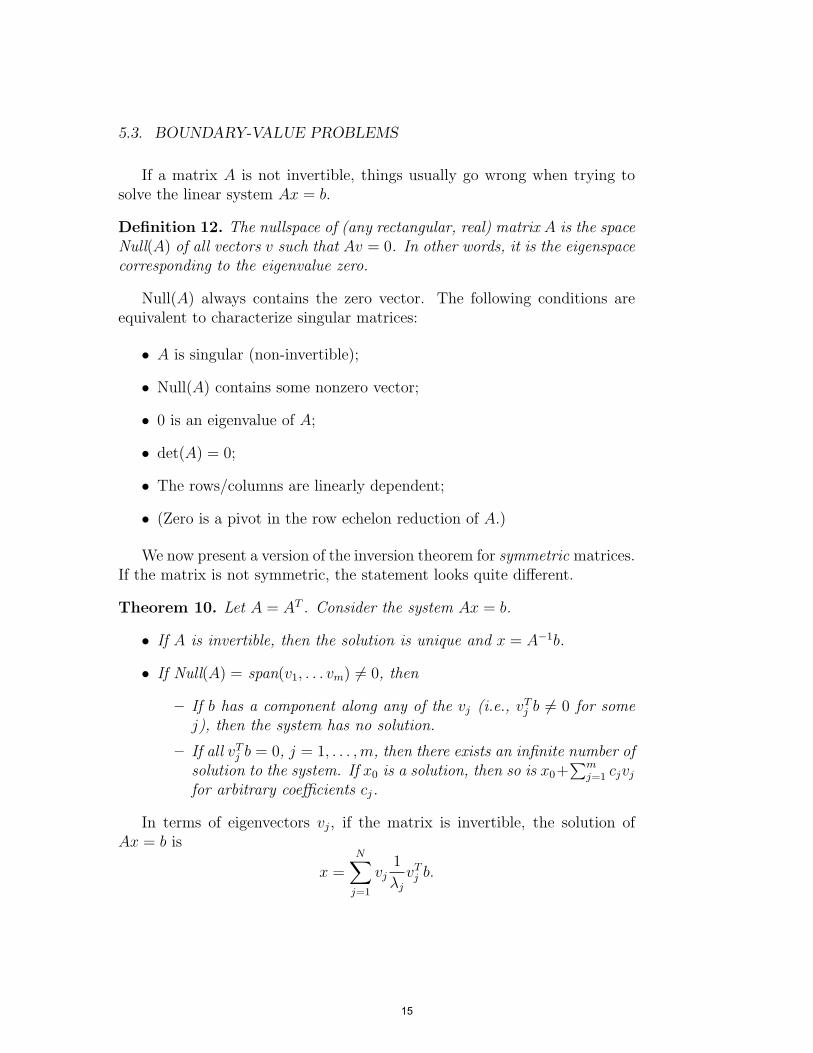
If a matrix A is not invertible, things usually go wrong when trying tosolve the linear system Ax = b.
Definition 12. The nullspace of (any rectangular, real) matrix A is the spaceNull(A) of all vectors v such that Av = 0. In other words, it is the eigenspacecorresponding to the eigenvalue zero.
Null(A) always contains the zero vector. The following conditions areequivalent to characterize singular matrices:
• A is singular (non-invertible);
• Null(A) contains some nonzero vector;
• 0 is an eigenvalue of A;
• det(A) = 0;
• The rows/columns are linearly dependent;
• (Zero is a pivot in the row echelon reduction of A.)
We now present a version of the inversion theorem for symmetric matrices.If the matrix is not symmetric, the statement looks quite different.
Theorem 10. Let A = AT . Consider the system Ax = b.
• If A is invertible, then the solution is unique and x = A−1b.
• If Null(A) = span(v1, . . . vm) = 0, then
– If b has a component along any of the vj (i.e., vTj b = 0 for somej), then the system has no solution.
– If all vTj b = 0, j = 1, . . . ,m, then there exists an infinite numbsolution to the system. If x0 is a solution, then so is x0+
∑ er ofmj=1 cjvj
for arbitrary coefficients cj.
In terms of eigenvectors vj, if the matrix is invertible, the solution ofAx = b is
N
x =∑ 1
vj vTλ j b.jj=1
6
6
15

CHAPTER 5. METHODS FOR ORDINARY DIFFERENTIAL EQUATIONS
If A is not invertible, but vTj b = 0 for all the eigenvectors vj, j = 1, . . . ,mcorresponding to the zero eigenvalue (as in the theorem above), then we stillhave
N
x =∑ m
1vj vTj b+
∑cjvj,
λjj=m+1 j=1
where the first sum only runs from m + 1 to N , and the coefficients cj arearbitrary. (Apply the matrix A to this equation to see that they disappear.)
If vTj b = 0, then the operation 1 vTj b would result in an infinity whenλj
λj = 0 — a crude reason to see why the system has no solution in that case.
5.3.2 Properties of the matrix K
We are now equipped to study the matrix K and its inverse. Recall that weare interested in controlling e = K−1τ to get the error from the LTE. Fromthe results in the previous section, we know that
‖e‖2 = ‖K−1τ‖2 ≤ ‖K−1‖2‖τ‖2.
Since K is a symmetric matrix,
‖K−1 1‖2 = max |λj(K−1)| = .j minj |λj(K)|
So it remains for us to understand the eigenvalues of K, and specifically toshow that the minimum eigenvalue (in absolute value) does not get too small.What we mean by this is that there should exist a number c > 0 such that
c < minj|λj(K)|,
independently of the grid spacing h (recall that the size of K and its entriesdepend on h.) Only in that case will we be able to conclude that ‖e‖ is ofthe same order of magnitude as ‖τ‖.
Note in passing that if τ = O(h2) then ‖τ3
‖2 = i τ2i will beO( 1h4) =
h
O(h /2), which is not very appealing. Instead, itvector 2-norm as
√is
∑common to mo
√dify the
‖τ‖2,h =
√h∑
τ 2i ,
i
6
16

5.3. BOUNDARY-VALUE PROBLEMS
so as to restore ‖τ‖ 22,h = O(h ) (note how h times the sum resembles an
integral quadrature.) In that case, we also expect ‖τ‖2,h = O(h2). Thereasoning with matrix 2-norms does not change one bit form this differentchoice of normalization.
Let us now study the eigenvalues and eigenvectors of K. The best wayto guess them is to notice that KU = F is a discretization of −u′′ = f withDirichlet boundary conditions. The eigenvalue problem
−v′′ = λv, v(0) = v(1) = 0,
has a solution in terms of sines: for each n ≥ 1, we have the pair
vn(x) = sin(nπx), λ = n2π2.
This analogy is very fruitful: the eigenvectors of K are precisely the vnsampled at xj = jh,
(n)vj = sin(nπjh), j = 1, . . . , N − 1, n = 1, . . . , N − 1.
(here n is the label index, and j is the component index.) It is straightforwardand a little tedious to check from trigonometric formulas that v(n) defined bythis formula are indeed eigenvectors, with eigenvalues
4λn = sin2 πnh
( ), n = 1, . . . , Nh2 2
− 1.
A Taylor expansion for small h shows that the minimum eigenvalue is λ1 =π2 +O(h2), and this O(h2) is positive, so that λ1 ≥ π2.
Note in passing that since K is symmetric, the eigenvectors are automat-ically orthogonal, hence there is a way to normalize them so that V TV = Iand V V T = I. Applying the matrix V T is called the discrete sine trans-form (DST), and applying the matrix V is called the inverse discrete sinetransform (IDST).
The formula for the eigenvalues has two important consequences:
• The matrix K is invertible, now that it is clear that all its eigenvaluesare positive. So setting up the discrete problem as KU = F makessense.
• Returning to the error bound, we can now conclude that ‖e‖2,h1
≤2‖τ 2
2,h = O(h ), establishing once and for all that the finite-differenceπ‖
method is second-order accurate for −u′′ = f with Dirichlet boundaryconditions.
17
CHAPTER 5. METHODS FOR ORDINARY DIFFERENTIAL EQUATIONS
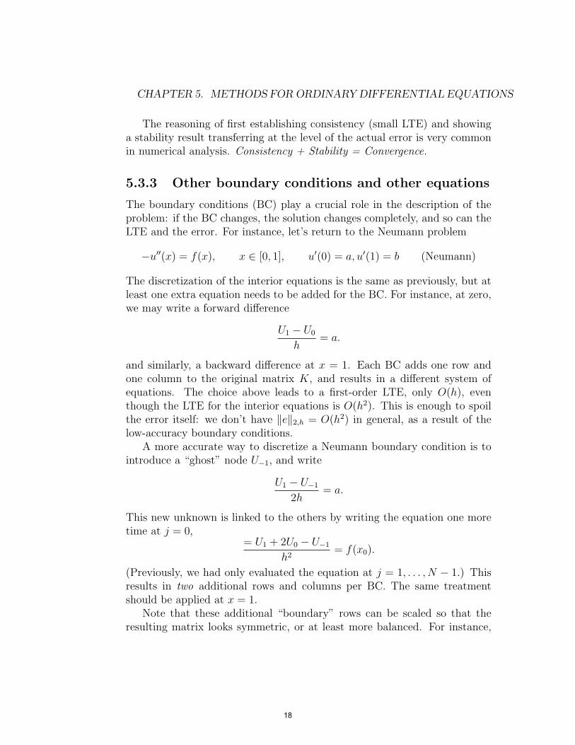
The reasoning of first establishing consistency (small LTE) and showinga stability result transferring at the level of the actual error is very commonin numerical analysis. Consistency + Stability = Convergence.
5.3.3 Other boundary conditions and other equations
The boundary conditions (BC) play a crucial role in the description of theproblem: if the BC changes, the solution changes completely, and so can theLTE and the error. For instance, let’s return to the Neumann problem
−u′′(x) = f(x), x ∈ [0, 1], u′(0) = a, u′(1) = b (Neumann)
The discretization of the interior equations is the same as previously, but atleast one extra equation needs to be added for the BC. For instance, at zero,we may write a forward difference
U1 − U0= a.
h
and similarly, a backward difference at x = 1. Each BC adds one row andone column to the original matrix K, and results in a different system ofequations. The choice above leads to a first-order LTE, only O(h), eventhough the LTE for the interior equations is O(h2). This is enough to spoilthe error itself: we don’t have ‖e‖2,h = O(h2) in general, as a result of thelow-accuracy boundary conditions.
A more accurate way to discretize a Neumann boundary condition is tointroduce a “ghost” node U−1, and write
U1 − U−1= a.
2h
This new unknown is linked to the others by writing the equation one moretime at j = 0,
= U1 + 2U0 − U−1= f(x0).
h2
(Previously, we had only evaluated the equation at j = 1, . . . , N − 1.) Thisresults in two additional rows and columns per BC. The same treatmentshould be applied at x = 1.
Note that these additional “boundary” rows can be scaled so that theresulting matrix looks symmetric, or at least more balanced. For instance,
18
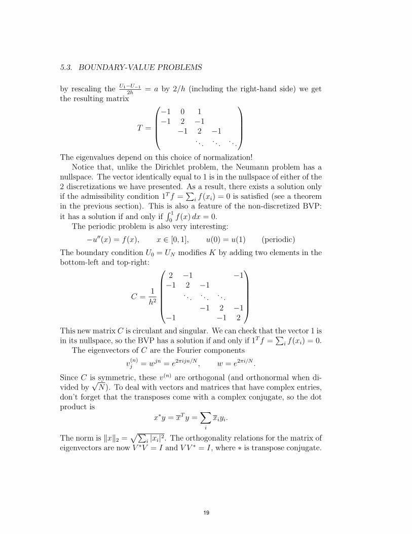
5.3. BOUNDARY-VALUE PROBLEMS
by rescaling the U1−U−1 = a by 2/h (including the right-hand side) we get2h
the resulting matrix −1 0 1
T =−1 2 −1 −1 2 −1
. . .. . .. . .
The eigenvalues depend on this choice of normalization!
Notice that, unlike the Dirichlet problem, the Neumann problem has anullspace. The vector identically equal to 1 is in the nullspace of either of the2 discretizations we have presented. ∑As a result, there exists a solution onlyif the admissibility condition 1Tf = i f(xi) = 0 is satisfied (see a theoremin the previous section). This is also a feature of the non-discretized BVP:
it has a solution if and only if∫ 1f(x) dx = 0.
0
The periodic problem is also very interesting:
−u′′(x) = f(x), x ∈ [0, 1], u(0) = u(1) (periodic)
The boundary condition U0 = UN modifies K by adding two elements in thebottom-left and top-right:
1 .C =
2 −1 −1−1 2
.−1
. . . .
h2
. . . −1 2 −1
−1 −1 2
This new matrix C is circulant and singular. We can chec
k that the vector 1 is
in its nullspace, so the BVP has a solution if and only if 1Tf = i f(xi) = 0.The eigenvectors of C are the Fourier components
(n)v = wjn = e2πijn/Nj , w = e2πi/N .
∑
Since C is symmetric, these v(n) are orthogonal (and orthonormal when di-vided by
√N). To deal with vectors and matrices that have complex entries,
don’t forget that the transposes come with a complex conjugate, so the dotproduct is
x∗y = xTy = xiyi.i
The norm is ‖x‖2 =√∑
i |xi|2. The orthogonalit
∑y relations for the matrix of
eigenvectors are now V ∗V = I and V V ∗ = I, where ∗ is transpose conjugate.
19

MIT OpenCourseWarehttp://ocw.mit.edu
18.330 Introduction to Numerical AnalysisSpring 2012
For information about citing these materials or our Terms of Use, visit: http://ocw.mit.edu/terms.