Chapter 5: Markov Chains - Aucklandfewster/325/notes/2011S2/ch5ann… · Chapter 5: Markov Chains...
27
83 Chapter 5: Markov Chains A.A.Markov 1856-1922 5.1 Introduction So far, we have examined several stochastic processes using transition diagrams and First-Step Analysis. The processes can be written as {X 0 ,X 1 ,X 2 ,...}, where X t is the state at time t. On the transition diagram, X t corresponds to which box we are in at step t. In the Gambler’s Ruin (Section 2.7), X t is the amount of money the gambler possesses after toss t. In the model for gene spread (Section 3.7), X t is the number of animals possessing the harmful allele A in generation t. The processes that we have looked at via the transition diagram have a crucial property in common: X t+1 depends only on X t . It does not depend upon X 0 ,X 1 ,...,X t−1 . Processes like this are called Markov Chains. Example: Random Walk (see Chapter 7) time t none of these steps matter for time t+1 ? ? time t+1 In a Markov chain, the future depends only upon the present: NOT upon the past.
Transcript of Chapter 5: Markov Chains - Aucklandfewster/325/notes/2011S2/ch5ann… · Chapter 5: Markov Chains...

83
Chapter 5: Markov Chains
A.A.Markov1856-1922
5.1 Introduction
So far, we have examined several stochastic processes usingtransition diagrams and First-Step Analysis.
The processes can be written as {X0, X1, X2, . . .},where Xt is the state at time t.
On the transition diagram, Xt corresponds to
which box we are in at step t.
In the Gambler’s Ruin (Section 2.7), Xt is the amount of money the gamblerpossesses after toss t. In the model for gene spread (Section 3.7), Xt is thenumber of animals possessing the harmful allele A in generation t.
The processes that we have looked at via the transition diagram have a crucial
property in common:Xt+1 depends only on Xt.
It does not depend upon X0, X1, . . . , Xt−1.
Processes like this are called Markov Chains.
Example: Random Walk (see Chapter 7)
time t
none of these steps matter for time t+1
?
? time t+1
In a Markov chain, the
future depends only
upon the present:
NOT upon the past.
84
.
.
.
.
.
.
.
.
.
.
..
.
.
....................................
.........................................................
.............................
.
.
.
.
.
.
.
.
.
..
.
.
....................................
..
.......................................................
............................
.
.
.
.
.
.
.
.
.
.
.
.
.
.
..
..................................
.........................................................
............................
.................................................................................................................................................
................
.
.
.
..
.
.
.
.
.
.
..
.
.
.
.
.
.
..
.
.
.
.
.
.
..
.
.
.
.
.
.
..
.
.
.
.
.
.
..
.
.
.
.
.
.
..
.
.
.
.
.
.
.
..
.
.
.
.
.
.
..
.
.
.
.
.
.
..
.
.
.
.
.
.
..
.
.
.
.
.
.
..
.
.
.
.
.
.
..
.
.
.
.
.
.
..
.
.
.
.
.
.
..
.
.
.
.
.
.
..
.
.
..
.
.
.
.
.
.
.
.
.
.
.
.
.
.
.
..
..............
.
.
.
..
.
.
.
.
.
.
..
.
.
.
.
.
.
..
.
.
.
.
.
.
..
.
.
.
.
.
.
..
.
.
.
.
.
.
..
.
.
.
.
.
.
..
.
.
.
.
.
.
..
.
.
.
.
.
.
..
.
.
.
.
.
.
.
..
.
.
.
.
.
.
..
.
.
.
.
.
.
..
.
.
.
.
.
.
..
.
.
.
.
.
.
..
.
.
.
.
.
.
..
.
.
.
.
.
.
..
.
.
.................
.
.
.
.
.
.
.
.
.
.
.
.
.
.
.
.
5 6
7
1 1
1..................................................
..
..
.
..
.
.
.
.
.
.
.
.
.
.
.
.
.
.
.
.
.
.
.
.
.
.
.
.
..........................
.............................
.
.
.
.
.
.
.
.
.
..
.
.
..
..................................
..
..
.
..
.
.
.
.
.
.
.
.
.
.
.
.
.
.
.
.
.
.
.
.
.
.
.
.
..........................
............................
.
.
.
.
.
.
.
.
.
.
.
.
.
.
..
..................................
.........................................................
............................
.................................................................................................................................................
................
.................................................................................................................................................
................
.
.
.
..
.
.
.
.
.
.
..
.
.
.
.
.
.
..
.
.
.
.
.
.
..
.
.
.
.
.
.
..
.
.
.
.
.
.
..
.
.
.
.
.
.
..
.
.
.
.
.
.
..
.
.
.
.
.
.
..
.
.
.
.
.
.
.
..
.
.
.
.
.
.
..
.
.
.
.
.
.
..
.
.
.
.
.
.
..
.
.
.
.
.
.
..
.
.
.
.
.
.
..
.
.
.
.
.
.
..
.
.
..
.
.
.
.
.
.
.
.
.
.
.
.
.
.
.
................
.
.
.
..
.
.
.
.
.
.
..
.
.
.
.
.
.
..
.
.
.
.
.
.
..
.
.
.
.
.
.
..
.
.
.
.
.
.
..
.
.
.
.
.
.
..
.
.
.
.
.
.
.
..
.
.
.
.
.
.
..
.
.
.
.
.
.
..
.
.
.
.
.
.
..
.
.
.
.
.
.
..
.
.
.
.
.
.
..
.
.
.
.
.
.
..
.
.
.
.
.
.
..
.
.
.
.
.
.
..
.
.
...
..............
.
.
.
.
.
.
.
.
.
.
.
.
.
.
.
.
3 2
4
13 1
23
1...................................................
..
..
.
.
.
.
.
.
.
.
.
.
.
.
.
.
.
.
.
.
.
.
.
.
.
.
..
.
..
...................................................
.........................................
............................
...............................................................................................
..
.
.
.
.
.
.
.
.
.
.
.
.
.
.
...............................................................................................
................
.
.
.
.
..
.
.
.
.
.
.
.
.
.
.
.
.
.
.
.
..
.
..
...........
135
15
15
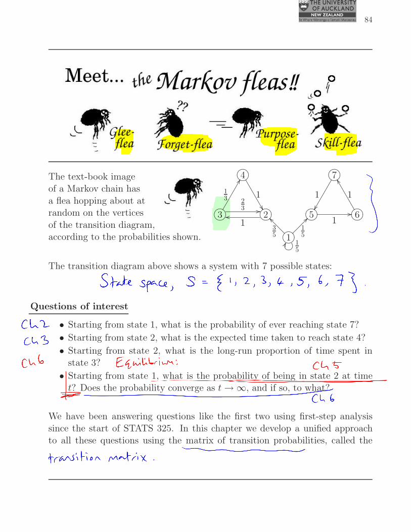
The text-book imageof a Markov chain has
a flea hopping about atrandom on the vertices
of the transition diagram,according to the probabilities shown.
The transition diagram above shows a system with 7 possible states:
state space S = {1, 2, 3, 4, 5, 6, 7}.
Questions of interest
• Starting from state 1, what is the probability of ever reaching state 7?
• Starting from state 2, what is the expected time taken to reach state 4?
• Starting from state 2, what is the long-run proportion of time spent instate 3?
• Starting from state 1, what is the probability of being in state 2 at timet? Does the probability converge as t → ∞, and if so, to what?
We have been answering questions like the first two using first-step analysis
since the start of STATS 325. In this chapter we develop a unified approachto all these questions using the matrix of transition probabilities, called thetransition matrix.
85
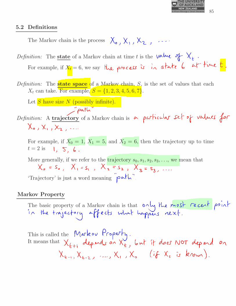
5.2 Definitions
The Markov chain is the process X0, X1, X2, . . ..
Definition: The state of a Markov chain at time t is the value of Xt.
For example, if Xt = 6, we say the process is in state 6 at time t.
Definition: The state space of a Markov chain, S, is the set of values that each
Xt can take. For example, S = {1, 2, 3, 4, 5, 6, 7}.
Let S have size N (possibly infinite).
Definition: A trajectory of a Markov chain is a particular set of values for
X0, X1, X2, . . ..
For example, if X0 = 1, X1 = 5, and X2 = 6, then the trajectory up to timet = 2 is 1, 5, 6.
More generally, if we refer to the trajectory s0, s1, s2, s3, . . ., we mean thatX0 = s0, X1 = s1, X2 = s2, X3 = s3, . . .
‘Trajectory’ is just a word meaning ‘path’.
Markov Property
The basic property of a Markov chain is that only the most recent pointin the trajectory affects what happens next.
This is called the Markov Property.
It means that Xt+1 depends upon Xt, but it does not depend upon Xt−1,. . . , X1, X0.
86
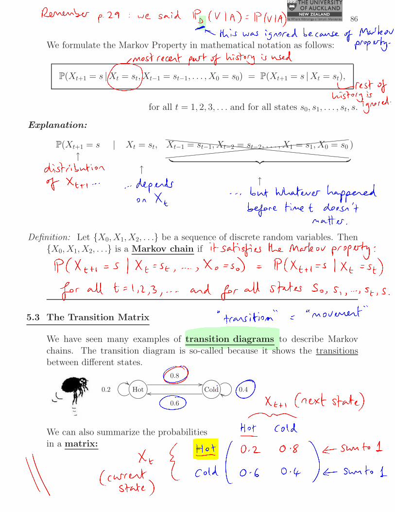
We formulate the Markov Property in mathematical notation as follows:
P(Xt+1 = s |Xt = st, Xt−1 = st−1, . . . , X0 = s0) = P(Xt+1 = s |Xt = st),
for all t = 1, 2, 3, . . . and for all states s0, s1, . . . , st, s.
Explanation:
P(Xt+1 = s | Xt = st, Xt−1 = st−1, Xt−2 = st−2, . . . , X1 = s1, X0 = s0 )↑ ︸ ︷︷ ︸
distribution ↑of Xt+1 depends ↑
on Xt but whatever happened before time tdoesn’t matter.
......................................................................................................................................................................................................................................................................................................................................................................................................................................................................................................................................................................................................................................................................................................................................................................................................................................................................................................................................................................................................................................................................................................................................................................................................................................................................................................................................................................................................................................................................................
Definition: Let {X0, X1, X2, . . .} be a sequence of discrete random variables. Then
{X0, X1, X2, . . .} is a Markov chain if it satisfies the Markov property:
P(Xt+1 = s |Xt = st, . . . , X0 = s0) = P(Xt+1 = s |Xt = st),
for all t = 1, 2, 3, . . . and for all states s0, s1, . . . , st, s.
5.3 The Transition Matrix
We have seen many examples of transition diagrams to describe Markov
chains. The transition diagram is so-called because it shows the transitionsbetween different states.
.
.
.
.
.
.
.
.
.
.
.
.
.
.
.
.
..
.
.
.
.
..
.
...........................................................
...........................................................................................
..................................................
.
.
.
.
.
.
.
.
.
.
.
.
.
.
.
..
.
.
.
.
..
.
...........................................................
...........................................................................................
.................................................
.
......................................
...................................................................
.........
...................................................................................................................
.........................
.
..
..
.
..
.
.
.
.
.
.
.
.
.
........................
..
..
.
..
.
.
.
..
.
.
.
.
......................................................................................................................................................................................................................................
................
......................................................................................................................................................................................................................................
................
0.40.2
0.8
0.6
Hot Cold
We can also summarize the probabilitiesin a matrix:
(0.2 0.8
0.6 0.4
){Hot
ColdXt
Hot Cold
︷ ︸︸ ︷
Xt+1
87
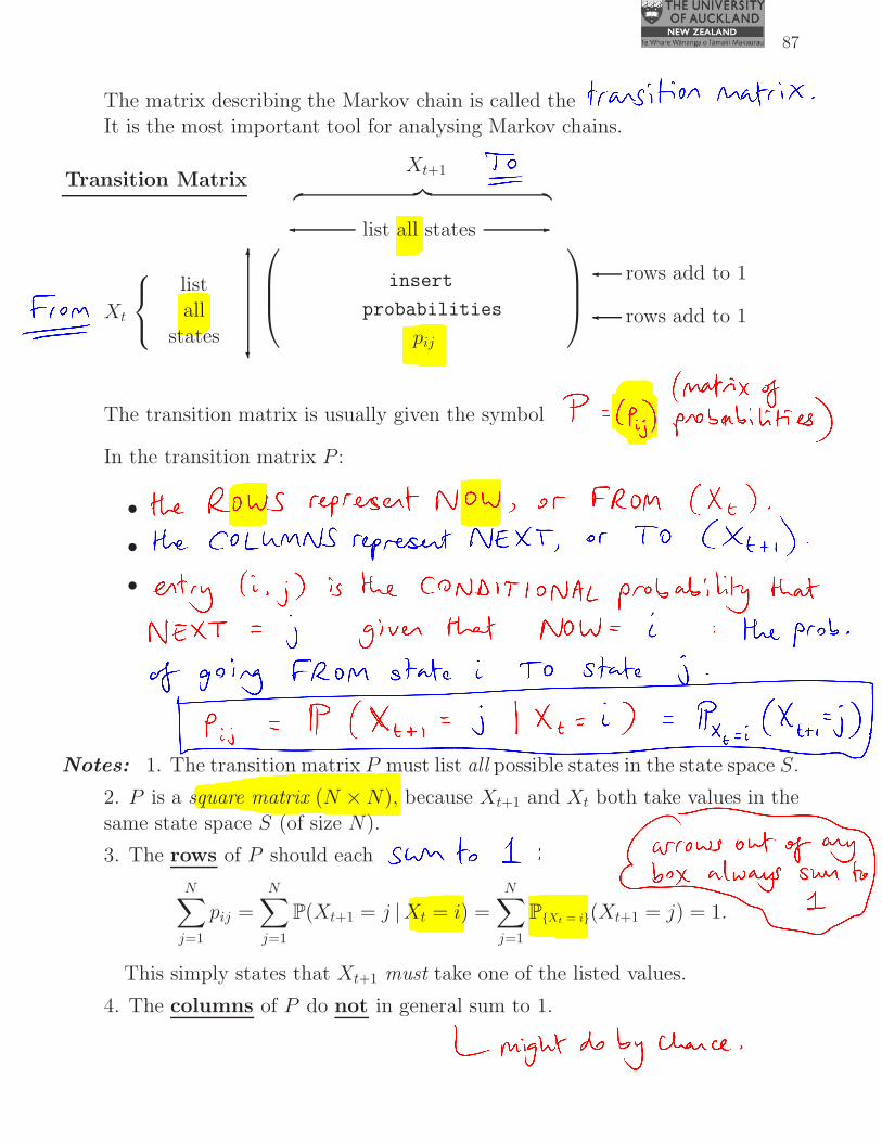
The matrix describing the Markov chain is called the transition matrix.It is the most important tool for analysing Markov chains.
Transition Matrix
listall
statesXt
list all states -�
︷ ︸︸ ︷
Xt+1
?
6
insert
probabilities
pij
rows add to 1�
rows add to 1�
The transition matrix is usually given the symbol P = (pij).
In the transition matrix P :
• the ROWS represent NOW, or FROM (Xt);
• the COLUMNS represent NEXT, or TO (Xt+1);
• entry (i, j) is the CONDITIONAL probability that NEXT = j,given that NOW = i: the probability of going FROM state i TO
state j.
pij = P(Xt+1 = j |Xt = i).
Notes: 1. The transition matrix P must list all possible states in the state space S.
2. P is a square matrix (N × N), because Xt+1 and Xt both take values in the
same state space S (of size N).
3. The rows of P should each sum to 1:
N∑
j=1
pij =N∑
j=1
P(Xt+1 = j |Xt = i) =N∑
j=1
P{Xt = i}(Xt+1 = j) = 1.
This simply states that Xt+1 must take one of the listed values.
4. The columns of P do not in general sum to 1.

88
Definition: Let {X0, X1, X2, . . .} be a Markov chain with state space S, where Shas size N (possibly infinite). The transition probabilities of the Markov
chain are
pij = P(Xt+1 = j |Xt = i) for i, j ∈ S, t = 0, 1, 2, . . .
Definition: The transition matrix of the Markov chain is P = (pij).
5.4 Example: setting up the transition matrix
We can create a transition matrix for any of the transition diagrams we haveseen in problems throughout the course. For example, check the matrix below.
Example: Tennis game at Deuce.VENUS
WINS (W)VENUS
AHEAD (A)
VENUSBEHIND (B)
p
q
p p
VENUSLOSES (L)
DEUCE (D)
D A B W LDA
BWL
0 p q 0 0q 0 0 p 0
p 0 0 0 q0 0 0 1 00 0 0 0 1
5.5 Matrix Revision
Notation
col j
aijrow i
NN by
A
Let A be an N × N matrix.
We write A = (aij),i.e. A comprises elements aij.
The (i, j) element of A is written both as aij and (A)ij:e.g. for matrix A2 we might write (A2)ij.

89
Matrix multiplication=
Let A = (aij) and B = (bij)be N × N matrices.
The product matrix is A × B = AB, with elements (AB)ij =
N∑
k=1
aikbkj.
Summation notation for a matrix squared
Let A be an N × N matrix. Then
(A2)ij =N∑
k=1
(A)ik(A)kj =N∑
k=1
aikakj.
Pre-multiplication of a matrix by a vector
Let A be an N×N matrix, and let π be an N×1 column vector: π =
π1...
πN
.
We can pre-multiply A by πT to get a 1 × N row vector,πTA =
((πTA)1, . . . , (π
TA)N
), with elements
(πTA)j =N∑
i=1
πiaij.
5.6 The t-step transition probabilities
Let {X0, X1, X2, . . .} be a Markov chain with state space S = {1, 2, . . . , N}.
Recall that the elements of the transition matrix P are defined as:
(P )ij = pij = P(X1 = j |X0 = i) = P(Xn+1 = j |Xn = i) for any n.
pij is the probability of making a transition FROM state i TO state j in a
SINGLE step.
Question: what is the probability of making a transition from state i to state j
over two steps? I.e. what is P(X2 = j |X0 = i)?


90
We are seeking P(X2 = j |X0 = i). Use the Partition Theorem:
P(X2 = j |X0 = i) = Pi(X2 = j) (notation of Ch 2)
=
N∑
k=1
Pi(X2 = j |X1 = k)Pi(X1 = k) (Partition Thm)
=N∑
k=1
P(X2 = j |X1 = k, X0 = i)P(X1 = k |X0 = i)
=
N∑
k=1
P(X2 = j |X1 = k)P(X1 = k |X0 = i)
(Markov Property)
=N∑
k=1
pkjpik (by definitions)
=
N∑
k=1
pikpkj (rearranging)
= (P 2)ij. (see Matrix Revision)
The two-step transition probabilities are therefore given by the matrix P 2:
P(X2 = j |X0 = i) = P(Xn+2 = j |Xn = i) =(P 2
)
ijfor any n.
3-step transitions: We can find P(X3 = j |X0 = i) similarly, but conditioning on
the state at time 2:
P(X3 = j |X0 = i) =N∑
k=1
P(X3 = j |X2 = k)P(X2 = k |X0 = i)
=N∑
k=1
pkj
(P 2
)
ik
= (P 3)ij.
91
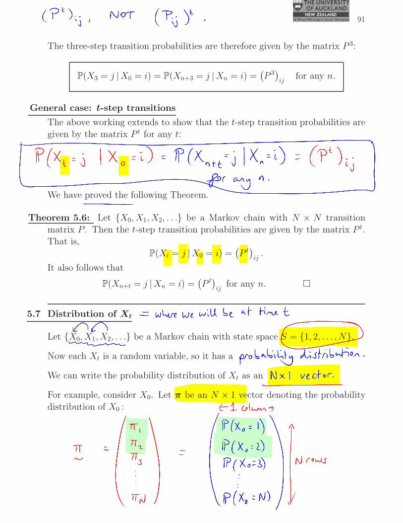
The three-step transition probabilities are therefore given by the matrix P 3:
P(X3 = j |X0 = i) = P(Xn+3 = j |Xn = i) =(P 3
)
ijfor any n.
General case: t-step transitions
The above working extends to show that the t-step transition probabilities are
given by the matrix P t for any t:
P(Xt = j |X0 = i) = P(Xn+t = j |Xn = i) =(P t
)
ijfor any n.
We have proved the following Theorem.
Theorem 5.6: Let {X0, X1, X2, . . .} be a Markov chain with N × N transition
matrix P . Then the t-step transition probabilities are given by the matrix P t.That is,
P(Xt = j |X0 = i) =(P t
)
ij.
It also follows that
P(Xn+t = j |Xn = i) =(P t
)
ijfor any n. �
5.7 Distribution of Xt
Let {X0, X1, X2, . . .} be a Markov chain with state space S = {1, 2, . . . , N}.
Now each Xt is a random variable, so it has a probability distribution.
We can write the probability distribution of Xt as an N × 1 vector.
For example, consider X0. Let π be an N × 1 vector denoting the probability
distribution of X0 :
π =
π1
π2...
πN
=
P(X0 = 1)P(X0 = 2)
...P(X0 = N)
92
In the flea model, this corresponds to the flea choosing at random whichvertex it starts off from at time 0, such that
P(flea chooses vertex i to start) = πi.
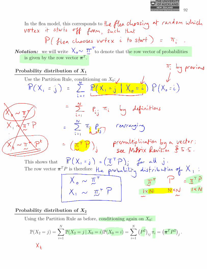
Notation: we will write X0 ∼ πT to denote that the row vector of probabilitiesis given by the row vector πT .
Probability distribution of X1
Use the Partition Rule, conditioning on X0:
P(X1 = j) =
N∑
i=1
P(X1 = j |X0 = i)P(X0 = i)
=
N∑
i=1
pijπi by definitions
=N∑
i=1
πipij
=(πTP
)
j.
(pre-multiplication by a vector from Section 5.5).
This shows that P(X1 = j) =(πTP
)
jfor all j.
The row vector πTP is therefore the probability distribution of X1:
X0 ∼ πT
X1 ∼ πTP.
Probability distribution of X2
Using the Partition Rule as before, conditioning again on X0:
P(X2 = j) =N∑
i=1
P(X2 = j |X0 = i)P(X0 = i) =N∑
i=1
(P 2
)
ijπi =
(πTP 2
)
j.

93
The row vector πTP 2 is therefore the probability distribution of X2:
X0 ∼ πT
X1 ∼ πTP
X2 ∼ πTP 2
...
Xt ∼ πTP t.
These results are summarized in the following Theorem.
Theorem 5.7: Let {X0, X1, X2, . . .} be a Markov chain with N × N transitionmatrix P . If the probability distribution of X0 is given by the 1×N row vectorπT , then the probability distribution of Xt is given by the 1 × N row vector
πTP t. That is,X0 ∼ πT ⇒ Xt ∼ πTP t.
Note: The distribution of Xt is Xt ∼ πTP t.The distribution of Xt+1 is Xt+1 ∼ πTP t+1.
Taking one step in the Markov chain corresponds to multiplying by P onthe right.
Note: The t-step transition matrix is P t (Theorem 5.6).
The (t + 1)-step transition matrix is P t+1.Again, taking one step in the Markov chain corresponds to multiplying by P
on the right.

94
5.8 Trajectory Probability
.
.
.
.
.
.
.
.
.
.
.
.
..
.
....................................
........................................................
.............................
.
.
.
.
.
.
.
.
.
.
.
..
.
....................................
........................................................
............................
.
.
.
.
.
.
.
.
.
.
.
.
..
.
..
..................................
..
..
.
.
.
.
.
.
.
.
.
.
.
.
.
.
.
.
.
.
.
.
.
.
.
.
.
..
..
...................................................
.................................................................................................................................................
................
..
.
.
.
.
.
.
..
.
.
.
.
.
.
..
.
.
.
.
.
.
..
.
.
.
.
.
.
..
.
.
.
.
.
.
..
.
.
.
.
.
.
..
.
.
.
.
.
.
.
..
.
.
.
.
.
.
..
.
.
.
.
.
.
..
.
.
.
.
.
.
..
.
.
.
.
.
.
..
.
.
.
.
.
.
..
.
.
.
.
.
.
..
.
.
.
.
.
.
..
.
.
.
.
.
.
..
.
.
.
.
.
..
.
.
.
.
.
.
.
.
.
.
.
.
.
.
.
.
...............
.
.
.
.
.
..
.
.
.
.
.
.
.
..
.
.
.
.
.
.
..
.
.
.
.
.
.
..
.
.
.
.
.
.
..
.
.
.
.
.
.
..
.
.
.
.
.
.
..
.
.
.
.
.
.
..
.
.
.
.
.
.
..
.
.
.
.
.
.
..
.
.
.
.
.
.
.
..
.
.
.
.
.
.
..
.
.
.
.
.
.
..
.
.
.
.
.
.
..
.
.
.
.
.
.
..
.
.
.
.
.
.
....
..............
.
.
.
.
.
.
.
.
.
.
.
.
.
.
.
.
5 6
7
1 1
1...................................................
..
..
.
.
.
.
.
.
.
.
.
.
.
.
.
.
.
.
.
.
.
.
.
.
.
.
.
..
.........................
.............................
.
.
.
.
.
.
.
.
.
.
.
..
.
....................................
..
..
.
.
.
.
.
.
.
.
.
.
.
.
.
.
.
.
.
.
.
.
.
.
.
.
.
..
.........................
............................
.
.
.
.
.
.
.
.
.
.
.
.
..
.
..
..................................
..
..
.
.
.
.
.
.
.
.
.
.
.
.
.
.
.
.
.
.
.
.
.
.
.
.
.
..
..
...................................................
.................................................................................................................................................
................
.................................................................................................................................................
................
.
.
.
.
.
..
.
.
.
.
.
.
.
..
.
.
.
.
.
.
..
.
.
.
.
.
.
..
.
.
.
.
.
.
..
.
.
.
.
.
.
..
.
.
.
.
.
.
..
.
.
.
.
.
.
..
.
.
.
.
.
.
..
.
.
.
.
.
.
..
.
.
.
.
.
.
.
..
.
.
.
.
.
.
..
.
.
.
.
.
.
..
.
.
.
.
.
.
..
.
.
.
.
.
.
..
.
.
.
.
.
.
....
.
.
.
.
.
.
.
.
.
.
.
.
.
.
................
..
.
.
.
.
.
.
..
.
.
.
.
.
.
..
.
.
.
.
.
.
..
.
.
.
.
.
.
..
.
.
.
.
.
.
..
.
.
.
.
.
.
..
.
.
.
.
.
.
.
..
.
.
.
.
.
.
..
.
.
.
.
.
.
..
.
.
.
.
.
.
..
.
.
.
.
.
.
..
.
.
.
.
.
.
..
.
.
.
.
.
.
..
.
.
.
.
.
.
..
.
.
.
.
.
.
..
.
.
.
.
.
..
...............
.
.
.
.
.
.
.
.
.
.
.
.
.
.
.
.
3 2
4
13 1
23
1.................................................
..........................................................
............................
.
..
.
.
.
.
.
.
.
.
.
.
.
.
.
.
.
.
.
..
.
..............................................
...............................................................................................
.
.
.
..
.
.
.
.
.
.
.
.
.
.
.
...............................................................................................
................
.
.
.
.
..
.
.
.
.
.
.
.
.
.
.
.
.
.
.
.
.
.
..............
135
15
15
Recall that a trajectory is a sequence
of values for X0, X1, . . . , Xt.
Because of the Markov Property,we can find the probability of any
trajectory by multiplying togetherthe starting probability and allsubsequent single-step probabilities.
Example: Let X0 ∼ (34, 0,
14 , 0, 0, 0, 0). What is the probability of the trajectory
1, 2, 3, 2, 3, 4?
P(1, 2, 3, 2, 3, 4) = P(X0 = 1) × p12 × p23 × p32 × p23 × p34
= 34× 3
5× 1 × 2
3× 1 × 1
3
= 110.
Proof in formal notation using the Markov Property:
Let X0 ∼ πT . We wish to find the probability of the trajectory s0, s1, s2, . . . , st.
P(X0 = s0, X1 = s1, . . . , Xt = st)
= P(Xt = st |Xt−1 = st−1, . . . , X0 = s0) × P(Xt−1 = st−1, . . . , X0 = s0)
= P(Xt = st |Xt−1 = st−1) × P(Xt−1 = st−1, . . . , X0 = s0) (Markov Property)
= pst−1,stP(Xt−1 = st−1 |Xt−2 = st−2, . . . , X0 = s0) × P(Xt−2 = st−2, . . . , X0 = s0)
...
= pst−1,st× pst−2,st−1
× . . . × ps0,s1× P(X0 = s0)
= pst−1,st× pst−2,st−1
× . . . × ps0,s1× πs0
.

95
5.9 Worked Example: distribution of Xt and trajectory probabilities
2
1 30.60.2
0.2
0.4
0.6
0.2
0.8
Purpose-flea zooms around
the vertices of the transitiondiagram opposite. Let Xt bePurpose-flea’s state at time t
(t = 0, 1, . . .).
(a) Find the transition matrix, P .
Answer:P =
0.6 0.2 0.2
0.4 0 0.6
0 0.8 0.2
(b) Find P(X2 = 3 |X0 = 1).
P(X2 = 3 |X0 = 1) =(P 2
)
13=
0.6 0.2 0.2
· · ·
· · ·
· · 0.2
· · 0.6
· · 0.2
= 0.6 × 0.2 + 0.2 × 0.6 + 0.2 × 0.2
= 0.28.
Note: we only need one element of the matrixP 2, so don’t lose exam time byfinding the whole matrix.
(c) Suppose that Purpose-flea is equally likely to start on any vertex at time 0.Find the probability distribution of X1.
From this info, the distribution ofX0 is πT =(
13,
13,
13
). We needX1 ∼ πTP .
πTP =(1
313
13)
0.6 0.2 0.2
0.4 0 0.6
0 0.8 0.2
=
(13
13
13
).
ThusX1 ∼(
13 ,
13 ,
13
)and thereforeX1 is also equally likely to be 1, 2, or 3.

96
(d) Suppose that Purpose-flea begins at vertex 1 at time 0. Find the probabilitydistribution of X2.
The distribution ofX0 is nowπT = (1, 0, 0). We needX2 ∼ πTP 2.
πTP 2 =
(1 0 0)
0.6 0.2 0.2
0.4 0 0.6
0 0.8 0.2
0.6 0.2 0.2
0.4 0 0.6
0 0.8 0.2
=
(0.6 0.2 0.2)
0.6 0.2 0.2
0.4 0 0.6
0 0.8 0.2
= (0.44 0.28 0.28) .
Thus P(X2 = 1) = 0.44, P(X2 = 2) = 0.28, P(X2 = 3) = 0.28.
Note that it is quickest to multiply the vector by the matrix first: we don’t need tocomputeP 2 in entirety.
(e) Suppose that Purpose-flea is equally likely to start on any vertex at time 0.Find the probability of obtaining the trajectory (3, 2, 1, 1, 3).
P(3, 2, 1, 1, 3) = P(X0 = 3) × p32 × p21 × p11 × p13 (Section 5.8)
= 13 × 0.8 × 0.4 × 0.6 × 0.2
= 0.0128.
97
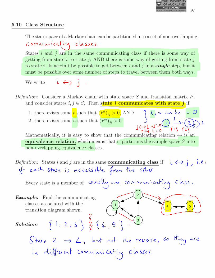
5.10 Class Structure
The state space of a Markov chain can be partitioned into a set of non-overlappingcommunicating classes.
States i and j are in the same communicating class if there is some way of
getting from state i to state j, AND there is some way of getting from state jto state i. It needn’t be possible to get between i and j in a single step, but itmust be possible over some number of steps to travel between them both ways.
We write i ↔ j.
Definition: Consider a Markov chain with state space S and transition matrix P ,
and consider states i, j ∈ S. Then state i communicates with state j if:
1. there exists some t such that (P t)ij > 0, AND
2. there exists some u such that (P u)ji > 0.
Mathematically, it is easy to show that the communicating relation ↔ is an
equivalence relation, which means that it partitions the sample space S intonon-overlapping equivalence classes.
Definition: States i and j are in the same communicating class if i ↔ j: i.e. if
each state is accessible from the other.
Every state is a member of exactly one communicating class.
2
3
4 51
Example: Find the communicatingclasses associated with thetransition diagram shown.
Solution:
{1, 2, 3}, {4, 5}.
State 2 leads to state 4, but state 4 does not lead back to state 2,so they are in different communicating classes.
98
Definition: A communicating class of states is closed if it is not possible toleave that class.
That is, the communicating class C is closed if pij = 0 whenever i ∈ C and
j /∈ C.
Example: In the transition diagram above:• Class {1, 2, 3} is not closed: it is possible to escape to class {4, 5}.
• Class {4, 5} is closed: it is not possible to escape.
Definition: A state i is said to be absorbing if the set {i} is a closed class.
.
.
.
.
.
.
.
.
.
.
.
.
.
.
.
.
.
.
.
..
.
.
................................
........................................................................................................................
.................................................
........................................
..
..
.
.
..
.
.
.
.
.
.
.
.
.
.
.
.
.
.
.
.
.
.
.
.
.
.
.
.
.
.
..
.
..
....................................
.........................
................
...........................................................................................................................
................
1i
Definition: A Markov chain or transition matrix P is said to be irreducible if
i ↔ j for all i, j ∈ S. That is, the chain is irreducible if the statespace S is a single communicating class.
5.11 Hitting Probabilities
We have been calculating hittingprobabilities for Markov chainssince Chapter 2, using First-Step
Analysis. The hitting probabilitydescribes the probability that the
Markov chain will ever reach somestate or set of states.
In this section we show how hitting
probabilities can be written in asingle vector. We also see a generalformula for calculating the hitting
probabilities. In general it is easierto continue using our own common
sense, but occasionally the formulabecomes more necessary.
99
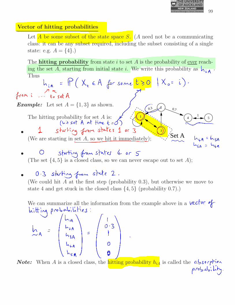
Vector of hitting probabilities
Let A be some subset of the state space S. (A need not be a communicating
class: it can be any subset required, including the subset consisting of a singlestate: e.g. A = {4}.)
The hitting probability from state i to set A is the probability of ever reach-
ing the set A, starting from initial state i. We write this probability as hiA.Thus
hiA = P(Xt ∈ A for some t ≥ 0 |X0 = i).
2
3
51 4
Set A
0.3 0.7
1
Example: Let set A = {1, 3} as shown.
The hitting probability for set A is:
• 1 starting from states 1 or 3(We are starting in set A, so we hit it immediately);
• 0 starting from states 4 or 5(The set {4, 5} is a closed class, so we can never escape out to set A);
• 0.3 starting from state 2
(We could hit A at the first step (probability 0.3), but otherwise we move tostate 4 and get stuck in the closed class {4, 5} (probability 0.7).)
We can summarize all the information from the example above in a vector ofhitting probabilities:
hA =
h1A
h2A
h3A
h4A
h5A
=
10.3
10
0
.
Note: When A is a closed class, the hitting probability hiA is called the absorp-tion probability.
100
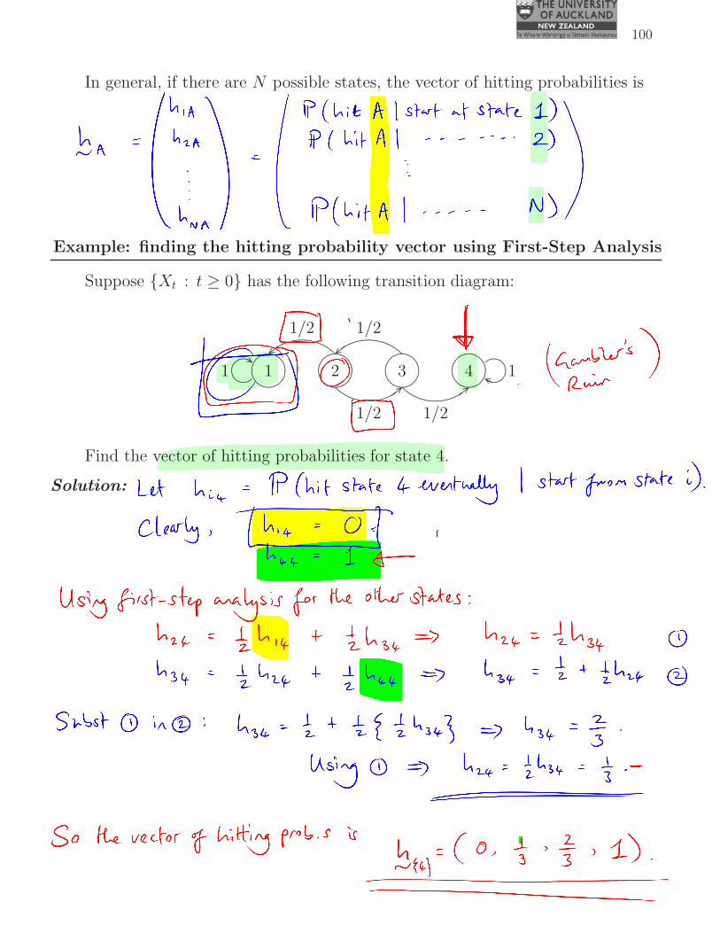
In general, if there are N possible states, the vector of hitting probabilities is
hA =
h1A
h2A...
hNA
=
P(hit A starting from state 1)P(hit A starting from state 2)
...P(hit A starting from state N)
.
Example: finding the hitting probability vector using First-Step Analysis
Suppose {Xt : t ≥ 0} has the following transition diagram:
.
.
.
.
.
.
.
.
.
.
.
.
.
.
.
.
.
.
.
.
..
.
..
..
......................................................
..............................................................................................
................................................. .
.
.
.
.
.
.
.
.
.
.
.
.
.
.
.
.
.
.
.
..
.
..........................................................
..............................................................................................
................................................. .
.
.
.
.
.
.
.
.
.
.
.
.
.
.
.
.
.
.
.
..
.
..
........................................................
..............................................................................................
................................................. .
.
.
.
.
.
.
.
.
.
.
.
.
.
.
.
.
.
.
.
..
.
..
..
......................................................
..............................................................................................
.................................................1 2 3 4
.
..................................................................................................................
...................................
........................................
..
..
.
..
.
.
.
.
.
.
.
.
.
.
.
.
.
.
.
.
.
.
.
.
.
.
.
.
.
.
.
..
.
............................
..........
......................................
........................................................................
.....................................................................
.........................
.
.
.
.
.
.
.
..
.
.
............
..
.
.....................................................................
.....................................................................
.........................
.
.
.
.
.
.
.
..
.
.
............
.............................................................................................
................................................
....................................
............
.............................................................................................
................................................
....................................
............
1/21/2
1/2 1/2
1 1
Find the vector of hitting probabilities for state 4.
Solution:
Let hi4 = P(hit state 4, starting from state i). Clearly,
h14 = 0
h44 = 1
Using first-step analysis, we also have:
h24 = 12h34 + 1
2 × 0
h34 = 12
+ 12h24
Solving,
h34 = 12 + 1
2
(12h34
)⇒ h34 = 2
3. So also, h24 = 12h34 = 1
3.
So the vector of hitting probabilities is
hA =(0, 1
3 ,23 , 1
).

101
Formula for hitting probabilities
In the previous example, we used our common sense to state that h14 = 0.
While this is easy for a human brain, it is harder to explain a general rule thatwould describe this ‘common sense’ mathematically, or that could be used to
write computer code that will work for all problems.
Although it is usually best to continue to use common sense when solvingproblems, this section provides a general formula that will always work to finda vector of hitting probabilities hA.
Theorem 5.11: The vector of hitting probabilities hA = (hiA : i ∈ S) is theminimal non-negative solution to the following equations:
hiA =
1 for i ∈ A,∑
j∈S
pijhjA for i /∈ A.
The ‘minimal non-negative solution’ means that:
1. the values {hiA} collectively satisfy the equations above;2. each value hiA is ≥ 0 (non-negative);3. given any other non-negative solution to the equations above, say {giA}
where giA ≥ 0 for all i, then hiA ≤ giA for all i (minimal solution).
Example: How would this formula be used to substitute for ‘common sense’ in
the previous example?
.
.
.
.
.
.
.
.
.
.
.
.
.
..
.
..
..
......................................
..................................................................
................................. .
.
.
.
.
.
.
.
.
.
.
.
.
..
.
..
........................................
..................................................................
................................. .
.
.
.
.
.
.
.
.
.
.
.
.
..
.
..
........................................
..................................................................
................................. .
.
.
.
.
.
.
.
.
.
.
.
.
..
.
..........................................
..................................................................
.................................1 2 3 4
................................................................................
.
.............
..................
.............................
..
.
.
.
.
.
.
.
.
.
.
.
.
.
.
.
.
.
.
.
.
.
..
.....................
.....
..................................
...................................................................................................
.............................
............
...................................................................................................
.............................
............
.
..................................................................
................................
.
............................
............
.
..................................................................
................................
.
............................
............
1/21/2
1/2 1/2
1 1The equations give:
hi4 =
1 if i = 4,∑
j∈S
pijhj4 if i 6= 4.
Thus,h44 = 1
h14 = h14 unspecified! Could be anything!
h24 = 12h14 + 1
2h34
h34 = 12h24 + 1
2h44 = 1
2h24 + 1
2

102
Becauseh14 could be anything, we have to use the minimal non-negative value,which ish14 = 0.(Need to checkh14 = 0 does not forcehi4<0 for any otheri: OK.)
The other equations can then be solved to give the same answers as before. �
Proof of Theorem 5.11 (non-examinable):
Consider the equations hiA =
{
1 for i ∈ A,∑
j∈S pijhjA for i /∈ A.(⋆)
We need to show that:
(i) the hitting probabilities {hiA} collectively satisfy the equations (⋆);
(ii) if {giA} is any other non-negative solution to (⋆), then the hitting proba-bilities {hiA} satisfy hiA ≤ giA for all i (minimal solution).
Proof of (i): Clearly, hiA = 1 if i ∈ A (as the chain hits A immediately).
Suppose that i /∈ A. Then
hiA = P(Xt ∈ A for some t ≥ 1 |X0 = i)
=∑
j∈S
P(Xt ∈ A for some t ≥ 1 |X1 = j)P(X1 = j |X0 = i)
(Partition Rule)
=∑
j∈S
hjA pij (by definitions).
Thus the hitting probabilities {hiA} must satisfy the equations (⋆).
Proof of (ii): Let h(t)iA = P(hit A at or before time t |X0 = i).
We use mathematical induction to show that h(t)iA ≤ giA for all t, and therefore
hiA = limt→∞ h(t)iA must also be ≤ giA.
103
Time t = 0: h(0)iA =
{
1 if i ∈ A,
0 if i /∈ A.
But because giA is non-negative and satisfies (⋆),
{
giA = 1 if i ∈ A,
giA ≥ 0 for all i.
So giA ≥ h(0)iA for all i.
The inductive hypothesis is true for time t = 0.
Time t: Suppose the inductive hypothesis holds for time t, i.e.
h(t)jA ≤ gjA for all j.
Consider
h(t+1)iA = P(hit A by time t + 1 |X0 = i)
=∑
j∈S
P(hit A by time t + 1 |X1 = j)P(X1 = j |X0 = i)
(Partition Rule)
=∑
j∈S
h(t)jA pij by definitions
≤∑
j∈S
gjA pij by inductive hypothesis
= giA because {giA} satisfies (⋆).
Thus h(t+1)iA ≤ giA for all i, so the inductive hypothesis is proved.
By the Continuity Theorem (Chapter 2), hiA = limt→∞ h(t)iA.
So hiA ≤ giA as required. �
104
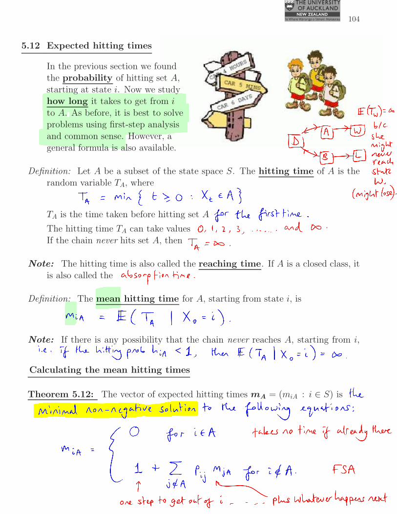
5.12 Expected hitting times
In the previous section we foundthe probability of hitting set A,
starting at state i. Now we studyhow long it takes to get from i
to A. As before, it is best to solveproblems using first-step analysis
and common sense. However, ageneral formula is also available.
Definition: Let A be a subset of the state space S. The hitting time of A is therandom variable TA, where
TA = min{t ≥ 0 : Xt ∈ A}.
TA is the time taken before hitting set A for the first time.
The hitting time TA can take values 0, 1, 2, . . ., and ∞.
If the chain never hits set A, then TA = ∞.
Note: The hitting time is also called the reaching time. If A is a closed class, itis also called the absorption time.
Definition: The mean hitting time for A, starting from state i, is
miA = E(TA |X0 = i).
Note: If there is any possibility that the chain never reaches A, starting from i,
i.e. if the hitting probability hiA < 1, then E(TA |X0 = i) = ∞.
Calculating the mean hitting times
Theorem 5.12: The vector of expected hitting times mA = (miA : i ∈ S) is the
minimal non-negative solution to the following equations:
miA =
0 for i ∈ A,
1 +∑
j /∈A
pijmjA for i /∈ A.
105
Proof (sketch):
Consider the equations miA =
{
0 for i ∈ A,
1 +∑
j /∈A pijmjA for i /∈ A.(⋆).
We need to show that:
(i) the mean hitting times {miA} collectively satisfy the equations (⋆);
(ii) if {uiA} is any other non-negative solution to (⋆), then the mean hitting
times {miA} satisfy miA ≤ uiA for all i (minimal solution).
We will prove point (i) only. A proof of (ii) can be found online at:
http://www.statslab.cam.ac.uk/~james/Markov/ , Section 1.3.
Proof of (i): Clearly, miA = 0 if i ∈ A (as the chain hits A immediately).
Suppose that i /∈ A. Then
miA = E(TA |X0 = i)
= 1 +∑
j∈S
E(TA |X1 = j)P(X1 = j |X0 = i)
(conditional expectation: take 1 step to get to state j
at time 1, then find E(TA) from there)
= 1 +∑
j∈S
mjA pij (by definitions)
= 1 +∑
j /∈A
pij mjA , because mjA = 0 for j ∈ A.
Thus the mean hitting times {miA} must satisfy the equations (⋆).�
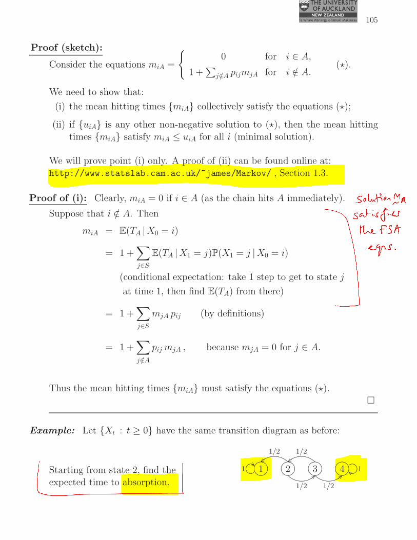
Example: Let {Xt : t ≥ 0} have the same transition diagram as before:
.
.
.
.
.
.
.
.
.
.
.
..
.
.
.
..
..
.....................................
..................................................................
.................................. .
.
.
.
.
.
.
.
.
.
.
..
.
.
.
..
.......................................
..................................................................
.................................. .
.
.
.
.
.
.
.
.
.
.
..
.
.
.
..
.......................................
..................................................................
.................................. .
.
.
.
.
.
.
.
.
.
.
..
.
.
.
.........................................
..................................................................
..................................1 2 3 4
....................
............................................................................................
.............................
..
.
.
.
.
.
.
.
.
.
.
.
.
.
.
.
.
.
.
.
.
.
..
.....................
.....
..................................
..................................................
.................................................
.............................
............
..................................................
.................................................
.............................
............
...................................................................
................................
.............................
............
...................................................................
................................
.............................
............
1/21/2
1/2 1/2
1 1Starting from state 2, find theexpected time to absorption.

106
Solution:
Starting from state i = 2, we wish to find the expected time to reachthe set A = {1, 4} (the set of absorbing states).
Thus we are looking for miA = m2A.
Now miA =
0 if i ∈ {1, 4},
1 +∑
j /∈A
pijmjA if i /∈ {1, 4}.
.
.
.
.
.
.
.
.
.
.
.
.
.
.
.
.
..
..
........................................
..
.
..
.
.
.
.
.
.
.
.
.
.
.
.
.
.
.
.
.
.
.
.
.
.
.
.
.
.
..
.
.
..
...........................
................................. .
.
.
.
.
.
.
.
.
.
.
.
.
.
.
.
..
..........................................
..
.
..
.
.
.
.
.
.
.
.
.
.
.
.
.
.
.
.
.
.
.
.
.
.
.
.
.
.
..
.
.
.............................
................................. .
.
.
.
.
.
.
.
.
.
.
.
.
.
.
.
..
..........................................
..
.
..
.
.
.
.
.
.
.
.
.
.
.
.
.
.
.
.
.
.
.
.
.
.
.
.
.
.
..
.
.
..
...........................
................................. .
.
.
.
.
.
.
.
.
.
.
.
.
.
.
.
............................................
..
.
..
.
.
.
.
.
.
.
.
.
.
.
.
.
.
.
.
.
.
.
.
.
.
.
.
.
.
..
.
.
..
...........................
.................................1 2 3 4
.
...............................................................................................................
.
............................
..
.
.
.
.
.
.
.
.
.
.
.
.
.
.
.
.
.
.
.
.
.
.
......................
.....
..................................
...................................................................................................
..................
.
.
.
.
.
.
.
.
.
.
.
............
...................................................................................................
..................
.
.
.
.
.
.
.
.
.
.
.
............
...................................................................
................................
.............................
............
...................................................................
................................
.............................
............
1/21/2
1/2 1/2
1 1Thus,m1A = 0 (because 1 ∈ A)
m4A = 0 (because 4 ∈ A)
m2A = 1 + 12m1A + 1
2m3A
⇒ m2A = 1 + 12m3A
m3A = 1 + 12m2A + 1
2m4A
= 1 + 12m2A
= 1 + 12
(1 + 1
2m3A
)
⇒ 34m3A = 3
2
⇒ m3A = 2.
Thus,m2A = 1 +
1
2m3A = 2.
The expected time to absorption is therefore E(TA) = 2 steps.

107
Example: Glee-flea hops around on a triangle. At each step he
moves to one of the other two vertices at random. What isthe expected time taken for Glee-flea to get from vertex 1
to vertex 2?
Solution:
transition matrix, P =
0 12
12
12 0 1
212
12 0
.
.
.
.
.
.
.
.
.
.
.
.
.
.
.
.
.
.
.
.
.
.
..
.
..
..
.......................................................
.............................................................................................
.................................................
.
.
.
.
.
.
.
.
.
.
.
.
.
.
.
.
.
.
.
.
..
.
...........................................................
.............................................................................................
................................................
.
.
.
.
.
.
.
.
.
.
.
.
.
.
.
.
.
.
..
.
.
..
.
...........................................................
...........................................................................................
.................................................
......................................................................................................................................................................................................................................
................
......................................................................................................................................................................................................................................
................
.
.
.
.
..
.
.
.
.
.
.
.
..
.
.
.
.
.
.
..
.
.
.
.
.
.
..
.
.
.
.
.
.
.
..
.
.
.
.
.
.
..
.
.
.
.
.
.
.
..
.
.
.
.
.
.
..
.
.
.
.
.
.
..
.
.
.
.
.
.
.
..
.
.
.
.
.
.
..
.
.
.
.
.
.
.
..
.
.
.
.
.
.
..
.
.
.
.
.
.
..
.
.
.
.
.
.
.
..
.
.
.
.
.
.
..
.
.
.
.
.
.
.
..
.
.
.
.
.
.
..
.
.
.
.
.
.
.
..
.
.
.
.
.
.
..
.
.
.
.
.
.
..
.
.
.
.
.
.
.
..
.
.
.
.
.
.
..
.
.
.
.
.
.
.
..
.
.
.
.
.
.
..
.
.
.
.
.
..
.
.
.
.
.
.
.
.
.
.
.
.
.
.
.
.
..
.............
.
.
.
.
.
.
..
.
.
.
.
.
.
..
.
.
.
.
.
.
.
..
.
.
.
.
.
.
..
.
.
.
.
.
.
..
.
.
.
.
.
.
.
..
.
.
.
.
.
.
..
.
.
.
.
.
.
.
..
.
.
.
.
.
.
..
.
.
.
.
.
.
.
..
.
.
.
.
.
.
..
.
.
.
.
.
.
..
.
.
.
.
.
.
.
..
.
.
.
.
.
.
..
.
.
.
.
.
.
.
..
.
.
.
.
.
.
..
.
.
.
.
.
.
..
.
.
.
.
.
.
.
..
.
.
.
.
.
.
..
.
.
.
.
.
.
.
..
.
.
.
.
.
.
..
.
.
.
.
.
.
..
.
.
.
.
.
.
.
..
.
.
.
.
.
.
..
.
.
.
.
.
.
.
..
.
.
.
..
...............
.
.
.
.
.
.
.
.
.
.
.
.
.
.
.
.
.
.
.
.
.
.
..
.
.
.
.
.
.
.
..
.
.
.
.
.
.
.
..
.
.
.
.
.
.
.
..
.
.
.
.
.
.
.
..
.
.
.
.
.
.
..
.
.
.
.
.
.
.
..
.
.
.
.
.
.
.
..
.
.
.
.
.
.
.
..
.
.
.
.
.
.
.
..
.
.
.
.
.
.
.
..
.
.
.
.
.
.
..
.
.
.
.
.
.
.
..
.
.
.
.
.
.
.
..
.
.
.
.
.
.
.
..
.
.
.
.
.
.
.
..
.
.
.
.
.
.
.
..
.
.
.
.
.
.
.
..
.
.
.
.
.
.
..
.
.
.
.
.
.
.
..
.
.
.
.
.
.
.
..
.
.
.
.
.
.
.
..
.
.
.
.
.
.
.
..
.
.
.
.
.
.
.
..
.
.
.
.
.
.
..
.
.
.
.
.
.
.
..
.
.
.
.
.
.
.
..
.
.
.
.
.
.
.
..
.
..
.
.
.
.
.
.
.
.
.
.
.
.
.
.
.
................
.
.
..
.
.
.
.
.
.
.
..
.
.
.
.
.
.
.
..
.
.
.
.
.
.
..
.
.
.
.
.
.
.
..
.
.
.
.
.
.
.
..
.
.
.
.
.
.
.
..
.
.
.
.
.
.
.
..
.
.
.
.
.
.
.
..
.
.
.
.
.
.
..
.
.
.
.
.
.
.
..
.
.
.
.
.
.
.
..
.
.
.
.
.
.
.
..
.
.
.
.
.
.
.
..
.
.
.
.
.
.
.
..
.
.
.
.
.
.
.
..
.
.
.
.
.
.
..
.
.
.
.
.
.
.
..
.
.
.
.
.
.
.
..
.
.
.
.
.
.
.
..
.
.
.
.
.
.
.
..
.
.
.
.
.
.
.
..
.
.
.
.
.
.
..
.
.
.
.
.
.
.
..
.
.
.
.
.
.
.
..
.
.
.
.
.
.
.
..
.
.
.
.
.
.
.
..
.
.
.
.
.
.
.
..
.
.
.
.
.
..
..
.............
.
.
.
.
.
.
.
.
.
.
.
.
.
.
.
.
2 3
1
1/2 1/21/2 1/2
1/2
1/2
We wish to findm12.
Now mi2 =
0 if i = 2,
1 +∑
j 6=2
pijmj2 if i 6= 2.
Thus
m22 = 0
m12 = 1 + 12m22 + 1
2m32 = 1 + 1
2m32.
m32 = 1 + 12m22 + 1
2m12
= 1 + 12m12
= 1 + 12
(1 + 1
2m32
)
⇒ m32 = 2.
Thus m12 = 1 + 12m32 = 2 steps.