CHAPTER 5 MACHINERY, EQUIPMENT, AND BUILDINGS: OPERATING COSTS

5-1

CHAPTER 5

MACHINERY, EQUIPMENT, AND BUILDINGS:OPERATING COSTS

INTRODUCTION

Types of Costs Associated with Machinery, Equipment, and Buildings

The ownership and use of machinery, equipment, and buildings leads to a variety of costs. Duringa given production period, the owner of these assets incurs costs associated with (1) holding each asset overthe period (including opportunity interest), (2) service reduction due to use and time, (3) changes in theimplicit value of the assets’ services, (4) maintenance, (5) service enhancement, and (6) the passage of timesuch as property tax and insurance. In Chapter 2 these costs were summarized using equation 2.25 as follows:

Service enhancement costs are in parentheses because they are usually handled in conjunction with servicereduction costs or the price change adjustments. Expenditures for maintenance and other time costs ofteninvolve the use of expendable inputs such as lubricants, parts, hired services, or operator labor. Thus theyare often estimated in conjunction with other operating costs such as seed, fertilizer, and supplies. Costsassociated with machinery, equipment, and buildings—such as opportunity interest and changes in servicecapacity or price—are often implicit and/or accrue over the life of the asset. Chapter 6 on durables addressesthese costs, whereas this chapter specifically discusses the operating costs associated with machinery,equipment, and buildings.

Determining Input-Output Relationships for Machinery, Buildings, and Equipment

As discussed in Chapter 2, capital assets are one of the types of inputs used in the production ofagricultural output. In assessing the cost of using alternative capital assets, it is useful to determine the outputper unit of input in order to assess the productivity of alternative production systems. If the productionsystem is of the Leontief type with fixed coefficients, then the output associated with a given asset is alsofixed. In this case, the cost per unit of input can be used to compute the cost per unit of output using theconstant technical coefficients. For example, if it is assumed that sweet corn production in centralWashington uses 2.77 hours of tractor time per acre and the total cost per hour for using the tractor iscomputed to be $23.80 with yields per acre of 9.5 tons, the cost per ton for the tractor is [(2.77)(23.80)/(9.5)]= $6.94. This assumes that an hour of tractor time has the same productivity regardless of the tractor age oruse per year. If the service output for the tractor varies with age or use, a more complicated procedure as

Chapter 5. Machinery, Equipment, and Buildings: Operating Costs

5-2

discussed in Appendix 6A is needed. In analyzing operating costs associated with machinery, equipment,and buildings in this chapter, it will be assumed that it is reasonable to compute cumulative maintenance andother operating costs for these items based on total lifetime hours of use and then to convert these to aconstant real cost per hour (day, year, etc.) of equally productive service, regardless of when that service isused within the economic life of the asset.

MACHINERY OPERATING COSTS

Methods to Estimate Machinery Operating Costs

There are two major methods of determining machinery operating expenses: producer surveys anddirect estimation using equations based on survey information. Surveys of individual farms are generallyused to calculate the costs and returns (CARs) of a specific commodity on a specific farm given the croppingmix and machinery set used on that farm. Where possible, surveys request producers to estimate machinerycosts for an enterprise. Many producers, however, do not have adequate enterprise records to identify costsby enterprise. When producers do not have adequate records, it is necessary to allocate whole-farm costs tothe individual enterprises. The allocation of whole-farm data to a specific enterprise is carried out in a varietyof methods. These include percentage allocations by each producer, allocations based on machinery use oneach enterprise, and allocations based on predetermined formulas. More discussion of these allocation issuesis contained in Chapters 6 and 9.

Direct estimation of machinery operating costs utilizes previously estimated engineering equations.Costs are estimated using typical machinery hours, age, size, and type. This information is usually based onexpert opinion, a consensus of selected producers, or a producer panel. Equations developed by agriculturalengineers and economists are then used to calculate typical costs for production in a specific region takinginto account typical machine usage and variations in the machinery complement used. The survey methodand engineering method are not mutually exclusive and are sometimes combined. For example, surveys maybe used to collect data on machinery use and size, which are then used with engineering equations to calculatecosts. Engineering equations are also used with the survey method as a means of allocating whole- farm coststo specific enterprises. A disadvantage of engineering equations is that they do not fully account for uniquefarm characteristics such as the level of management. The level of management can impact machinery costssignificantly, and can be important when making comparisons between a farm and regional averages.

The selection of which method or combination of methods to use in determining machinery repairor fuel use depends on a number of factors. Of major importance is the intended use of the cost estimates.The survey method is generally preferred when actual farm-level cost data are required. Actual farm-levelcost data are often required when the estimates are used for policy analysis and program administrationpurposes. Policy analysis often examines the variability in returns and how different policies may impactdifferent groups of farms by size and other variables. Policy analysis related to farm income issues isgenerally concerned with historical CARs that are best estimated with the survey method. In programadministration and program evaluation, actual data from individual farms are often needed, thereby makingthe survey approach the most appropriate. However, even in the “Agricultural Resource Management Study”(formerly FCRS) conducted by the United States Department of Agriculture (USDA) Economic ResearchService (ERS), total farm costs must be disaggregated by proportioning machinery costs to particularenterprises and, if needed, to particular field operations. This allocation is often accomplished using


5-3

equations originally published by Bowers and Hunt. Another potential benefit of the survey method is thatit permits farmers to compare their results against those of a group of farmers in a similar region.

Some uses of CAR estimates encompass situations where it is desirable to estimate machinery costsusing engineering equations, such as when CARs are being projected for a specified farm organization on atypical or representative farm in a region. In other cases, such as for new machinery, survey information maynot be available, making it necessary to use engineering equations. Engineering equations may be mostappropriate for technology assessments which call for potential changes in machinery complements. Also,the equations are particularly useful for making quick comparisons between machinery alternatives foraccomplishing a selected task.

In addition to the uses of the CAR estimates, there are a number of other factors one must considerin developing these estimates. Of importance are the resources which are available. The survey method hasa disadvantage compared to the use of equations in that it can be expensive in both dollars and humanresources required and the results obtained are tied to a point in time. Surveys are time consuming, makingit difficult to have information available on a timely basis. Other problems such as sampling and nonsamplingerrors can impact the results of the survey approach. The engineering approach generally is inexpensive anddoes not require a large time commitment. A disadvantage of the engineering approach is that some of theengineering equations have not recently been updated, which may impact the accuracy of the results.However, because the equations often use machine list price as a parameter, the cost estimates can be adjustedfor time by updating list price, fuel price, and so forth. There is and will continue to be an ongoing debateabout which is more accurate and appropriate—survey or direct machinery cost estimation.

In comparing estimates from different sources, it is important to know which methods were used incalculating the costs. Direct comparisons between estimates based on the survey approach and theengineering approach are not possible. The most appropriate method to use will depend largely on the useof the estimates. Whatever method is used, information on how the costs are estimated must be provided tothe potential user. For the survey method it is important to specify how, when, and where costs werecollected and calculated. If whole-farm costs were allocated to a specific commodity, the allocation methodshould be reported. The collection of whole-farm data in the survey method is recommended even ifallocations are not made on whole-farm costs. Whole-farm costs, at the very least, provide a useful checkto verify commodity-specific costs. If engineering equations are used, details about the machinerycomplement and farm machinery use should be specified.

Using Surveys to Estimate Machinery Operating Costs

Surveying farmers to elicit their machinery operating costs by enterprise is a challenging task becausemost farmers do not maintain records for this purpose. Farmers usually only record income and expenseinformation. To determine enterprise costs, either additional information necessary to allocate expenses toeach enterprise of interest must be obtained, or machinery costs for each enterprise must be elicited directly.

The first method of surveying machinery costs assumes that costs of machinery operation areavailable at the farm level. Expenses for fuel, lubrication, repairs, and so forth for the entire unit can usuallybe obtained from farm account books, income tax returns, or other financial statements. In addition,information necessary to allocate the farm-level costs to the enterprises of interest must also be elicited. Theadditional information may either be objective data, such as acres of various crops and units of livestock, or


5-4

(5.1)

various subjective factors, such as the operator's assessment of enterprise shares. If the producer does nothave or remember detailed information on tillage operations associated with each activity, then estimationbased on machine operations may be difficult. The use of a tableau similar to Figure 5.1 and /or the onediscussed in detail in Chapter 9 may be helpful in the subjective allocation of machine time and machinecosts.

The purpose of the top half of the tableau is to help the farm operator recall the acreages and machineoperations associated with each enterprise. The operator may not be able to fill in all the information, but themore complete the information, the better will be the allocated estimates in the bottom half of the tableau.The top half may also be useful in determining the machine operations that are analyzed using engineeringequations. Total farm expenses for fuel, lubrication, and repairs would then be entered in the whole-farmcolumn. This data could come from available records and operator estimates of labor time involved in on-farm repairs. Repair expenses would then be allocated between tractors, combines, and implements (ifpossible), still in the whole-farm column. The purpose of allocating the repair expenses is to determine whichtypes of equipment have the most repairs. Total fuel, lubrication, and repairs could then be allocated acrossenterprises. For example, on a Great Plains small grain farm, fuel costs for wheat and barley enterprises mayeach be estimated by the farm operator to be 50% of whole-farm expenses. Or, on an Idaho alfalfa and barleyoperation with 50% acreage in each crop, the allocation of repairs may be 65% to the alfalfa and 35% to thebarley due to high repair costs for haying equipment. The column expense total could then be used in anenterprise-specific CAR.

An alternative to a subjective allocation by the producer, researcher, or farm management consultantis the use of a regression equation similar to

to estimate each enterprise share. The dependent variable yt represents the total farm-level cost for an itemsuch as fuel for the tth farm in the sample, whereas the independent variables x1t and x2t represent differentfarm enterprises (usually measured in acres produced). For example, there may be different crops on a grainfarm, or acres of crops and units of livestock on a combined crop/livestock farm. The coefficients of eachvariable are then interpreted as the respective cost of each unit. The intercept value $0 is defined to be thewhole-farm level cost that is unallocated to each enterprise. Use of this method does require variation in costsand enterprise quantities among farms.


5-5

Figure 5.1 Allocation of Machine Costs for a Crop Producer

Item Whole-Farm

Enterprise 1 Enterprise 2 Enterprise n

Total Acres

Acres plowed

Acres disced

Acres harrowed

Acres planted withplanter

Acres planted with drill

Acres baled

etc.

Total fuel expense

Total lubrication expense

Total repair costs

Repairs on tractors X X X

Repairs on combines X X X

Repairs on balers X X X

Repairs on planters X X X

etc. X X X

TOTAL EXPENSE Total Farm Tot. Ent. 1 Tot. Ent. 2 Tot. Ent. n

Notes: (1) The top half of the table is completed first.(2) The whole-farm column in the bottom half is completed next.(3) The allocations across enterprises for total fuel, lubrication, and repairs is completed last. Boxes with X are not filled in.


5-6

The second method for obtaining machinery operating costs is to use a direct survey. However, theseprocedures are more complex. Past efforts have ranged from asking farmers to specify each component ofcost directly to observing each farmer's actual usage of the resource involved. Asking farmers directly toreport fuel costs per acre or repair costs per head of livestock can be efficient from the researcher's perspectivebecause only minimal effort must be expended for data collection. However, the data obtained must bereviewed carefully to ensure that the farmers understand what is being asked of them and that the estimatesobtained are accurate. To assist farmers with this process, various logs can be devised to aid and remind themof the data collection process. The underlying data to support estimation of the agricultural engineeringequations described later were originally collected by this method. Observing farmers' direct usage ofresources is far more time consuming but removes any errors associated with farmers' direct reporting of thecosts. In either of these procedures, results and significance of the analysis are conditional on the samplinglevels and methods employed.

Using Equations to Estimate Machinery Operating Costs for Crop Enterprises

Field operations to be performed and the set of machines to be used must be specified before costscan be estimated using engineering equations. Accurate specification of machinery costs using equationsrequires that the following steps be performed.

Farm Specification

Items required to identify the farm include (a) number of acres of each crop to be grown, and (b)machine operations on each crop, including time period (month or week) of execution. Machinery operatingcosts per acre typically do not vary much based on the size of machine as long as the implements and tractorsare fairly well matched. However, the ownership costs can vary substantially depending on the size andannual use of equipment. Farms specializing on one crop may use farm equipment intensively for shortperiods of time, but may use the equipment relatively few hours per year causing ownership costs per acreto be high relative to diversified farms where machinery can be used on several crops over numerous timeperiods.

Machinery Selection

The set of machinery selected for a farm must be capable of performing all required tasks in a timelyfashion. Also, it would be desirable to have a complement that can provide the required services for relativelylow ownership costs. Developers of CAR estimates using machinery cost equations should always check thefeasibility of the machinery complement being considered. This may involve something as straight forwardas identifying the time period (month or week) where it appears that the greatest demands are being placedon the machinery complement and then determining the hours of use for each machinery item. Tractor hoursare probably the most critical in terms of excess use. One tool for checking the feasibility of a machinerycomplement is found in Kletke and Sestak where a spreadsheet template (MACHSEL) is used for checkingthe feasibility of a complement and estimating the expected costs for a complement given any particular farmsituation. The greatest difficulty with this kind of template and the engineering equations in general is theamount of information that must be provided about the farm, the farm organization, and the machinery to beused. (See also the last section of Chapter 6).


1 Standards: ASAE S495 (Dec 94), Uniform Terminology for Agricultural Machinery Management;ASAE Engineering Practice: ASAE EP496.2, Agricultural Machinery Management (Mar 94); ASAE Data:ASAE D497.3, Agricultural Machinery Management Data (Nov 96).

5-7

(5.2)

(5.3)

Engineering Equations for Estimating Machinery Repair Costs per Hour of Use

The American Society of Agricultural Engineers (ASAE) publishes procedures for estimating thecosts to own and operate farm machinery. These procedures have been revised several times over their 40-year history. The latest procedures are given in the 1997 ASAE Standards1. The functional forms for costestimation have changed over the years as well as the repair coefficients and length of life as machinerytechnology has improved. Rotz and Bowers give a good summary of the changes that have taken place inthe engineering equations over time. These procedures have evolved from their start in the late 1920s and’30s. In 1966 it was suggested that repair and maintenance costs be estimated as a function of machine ageexpressed as a percent of lifetime service hours.

whereAR = accumulated repair and maintenance as a percent of list priceX = accumulated use as a percent of lifetime hoursRF1, RF2 = repair factors.

Note that AR is a percentage that must be multiplied by the list price to obtain total accumulatedrepairs and maintenance. In the late 1960s and early ’70s the equations were changed after several studieswere completed on machinery repair costs. The following equation was developed from work by Bowers andHunt.

whereTAR = total accumulated repairs and maintenance (dollars)LP = list price (dollars)X = accumulated use as a percentage of lifetime hours (0 # X # 100)RP1 = repairs over useful life as a proportion of list price (RP1 $ 0)RP2, RP3 = paired constants providing shape to repair curve.


5-8

(5.4)

The coefficients RP2 and RP3 come in pairs which shape the distribution of repairs over the life of the

machine. The coefficient RP1 is defined by where TAR* is the value of equation 5.3 when the

machine is at the end of its useful life. If h denotes accumulated hours of use and LIFE = total machine

lifetime (hours), then . When h = LIFE, then X = 100. Using this information we can define

the relationship between RP2 and RP3 by evaluating 5.3 with h = LIFE. Specifically,

When working with the Bowers and Hunt repair equation, the RP2 and RP3 pairs reported in Table 5.1 mustbe used. The purpose of the pairs of coefficients is to allocate repairs over the life of the machine. Thefunction of RP2 and RP3 is to shape the repair cost curve. The total expected repairs over the lifetime of themachine as a proportion of the initial list price is given by the Bowers and Hunt RP1 factor and so long asRP1 does not change, the total repairs over the life of the machine will not change no matter which set of RP2and RP3 is used. As the RP3 factor (second column in Table 5.1) increases, repairs are moved towards theend of machine life. When the first pair of coefficients (.01 and 1.0) is used, repairs occur linearly over thelife of the machine.

In 1977, a major change occurred in the equations. They were converted from three repair factors(RPi) to two repair factors (RFi) by expressing machine age in thousands of hours rather than as a percentof lifetime hours. In 1987, Rotz created an even more generic model that was adopted by the ASAEStandards Committee. This model is the standard in the latest ASAE publications. This accepted model is

whereCrm = total accumulated repair and maintenance (dollars)P = machine list price in current dollarsh = accumulated use (hours)RF1, RF2 = repair and maintenance factors.

The exponent (RF2) in equation 5.4 is the same as the exponent (RP3) in equation 5.3. The prices P and LPare also the same. The relationship between the other variables can be found by setting TAR = Crm and usingthe fact that RP3 = RF2 and P = LP.


5-9

(5.5)

By solving for RF1 as follows:

and, since it is determined that

In summary, equation 5.4 (Rotz equation) is related to equation 5.3 (Bowers and Hunt equation) in thefollowing manner.

Bowers and Hunt RotzTAR Crm

LP P(RP1) (1,000/LIFE)RP3 RF1

RP3 RF2

For those who want to use the Bowers and Hunt three-factor equations, the Rotz RF2 can be used to calculatethe Bowers and Hunt RP2 as follows:

The Rotz equations do not allow users to control the way repair costs occur over the life of the machine asdo the Bowers and Hunt equations. They also do not allow the user to specify what repair costs are expectedto be over the life of the machine. Lifetime repairs as a proportion of list price can be obtained from the

relationship Because useful life is implicit in the Rotz equations, it is possible to

obtain the RF1 values in Table 5.2 using information on useful life, lifetime repairs as a proportion of list


5-10

price, and RF2. For the first tractor in Table 5.2 with lifetime repairs equal to 100% of list price, repairs asa portion of list price are

TABLE 5.1 Paired Values for Repair and Maintenance Coefficients RP2

and RP3 where

RP2 (Bowers & Hunt)RP3 (Bowers & Hunt)

or RF2 (Rotz)

.0100000 1.0

.0063096 1.1

.0039811 1.2

.0025119 1.3

.0015849 1.4

.0010000 1.5

.0006310 1.6

.0002512 1.7

.0001585 1.9

.0001000 2.0

.0000631 2.1

.0000398 2.2

.0000251 2.3

In summary, the Rotz equations are easier to apply because only hours of use and list price arenecessary to estimate the accumulated repairs. What is given up for this simplicity is the ability to vary totalexpected life (LIFE) and the amount of repairs expected over the life of the machine (Bowers & Hunt RP1).If users are willing to give up control of these parameters, then the Rotz equations are a useful simplification.


5-11

However, because of the wide diversity in climate, variation in field conditions, and perhaps perceiveddifferences in quality of workmanship in machine manufacture, the older Bowers and Hunt equations can beused because they will give identical results given the same assumptions while allowing more flexibility forusers who want it.

In 1991, Rotz and Bowers revised the repair factors (RF1, RF2) for some types of machinery.Estimated life was increased for tractors, planting equipment, and self-propelled harvesting equipment anddecreased for beet harvesting equipment and forage blowers. They also reduced the repair factors for selectedmachinery. These changes are included in the current ASAE Standards (ASAE D472.3 NOV 96, Table 3)and are summarized in Table 5.2.

The ASAE repair and maintenance procedure is designed to estimate all of the costs associated withrepair and maintenance. These include all replacement parts, materials, shop expenses, and labor. Work doneat a machinery dealership includes all of these costs. Repair work done on the farm should include a cost forthe farmer's labor as well as a cost for maintaining a shop. Repair and maintenance costs are highly variableand unpredictable as to time of occurrence. Actual repair and maintenance costs vary widely with standarddeviations likely exceeding the mean cost.

The ASAE equations are useful for predicting the average costs for repair and maintenance over thelife of the machine. These equations have been used to estimate costs that occur during a relatively shortperiod (one or two years), but it is not a recommended practice. Also, they should not be used to estimaterepair and maintenance costs for machinery used beyond the estimated life of the machine. For machinesused beyond their estimated hours of life, agricultural engineers recommend using the repair and maintenancecost estimated for the last year of expected life.

Converting Costs per Hour to Costs per Acre Using ASAE Standards

Field Performance

Field performance is needed to convert machinery costs per hour to a per acre or per unit basis. Thereare two methods for estimating performance. The first alternative is to obtain an estimate from the producerbased on past experience. The second alternative is to use engineering equations to estimate fieldperformance. For estimating costs of a specific field operation for a given producer, the first alternative ispreferred. When producer estimates are not available, or when a typical or average measure is required, thesecond alternative can be used.

Estimating costs on a per acre basis requires knowledge of the effective field capacity of implementsand self-propelled equipment. Effective field capacity is expressed as acres per hour for some machines (forexample, plows and planters) or tons per acre for others (for example, balers and forage harvesters). Theeffective field capacity is estimated from the field speed, implement working width, field efficiency, and unityield of the field for a given piece of machinery. Field speed is the average speed at which the functionalwork will be done in the field. For example, a farmer might average 4 mph plowing when the plow is actuallyin the soil. Implement working width is the measured width of the working portion of the machine. Forexample, for a planter it is the average row width times the number of rows. The ratio of effective fieldcapacity to theoretical field capacity is the field efficiency of a machine. The field efficiency is expressedas a percent and is used to account for a number of factors that influence field operations, including failure


5-12

to utilize the theoretical operating width of the machine, time lost turning, operator habits, fieldcharacteristics, and so forth. Travel to and from a field, repairs and maintenance, and daily service activitiesare not accounted for in the field efficiency coefficient.

Calculated area capacity is computed as follows:

(5.6)

whereCa = acres per hour calculated capacityS = implement speed in miles per hourW = measured width of the implement in feetEf = field efficiency, the ratio of effective accomplishment compared to theoretical

accomplishment, expressed in percent8.25 = 43,560 (square feet per acre) divided by 5,280 (feet per mile) = width of acre 1

mile long.

Example: One of the machines used on the Ben and Bev Dairyman Farm is a 19N tandemdisk. Ben estimates that he normally travels six miles per hour when disking. Table 5.2indicates that a disk normally operates at about 80% efficiency because of turning, and in-field travel time. Given this information the expected acres planted per hour is

The amount of product yield is used to estimate capacity for machinery such as balers that do notcover each square foot of the field. Calculated material capacity is computed as follows:

(5.7)

TABLE 5.2 Field Efficiency, Field Speed, Estimated Life, Total Life Repair Cost, and Repair Factors for Selected Machinery

Field Efficiency Field Speed Estimated LifeTotal LifeR&M Cost Repair Factors

Machine Range%

Typical%

Rangemph

Typicalmph

Rangekm/h

Typicalkm/h h

% of Listprice RF1 RF2

TRACTORS2 wheel drive & stationary 12,000 100 0.007 2.04 wheel drive & crawler 16,000 80 0.003 2.0TILLAGE & PLANTINGMoldboard plow 70-90 85 3.0-6.0 4.5 5.0-10.0 7.0 2,000 100 0.29 1.8Heavy-duty disk 70-90 85 3.5-6.0 4.5 5.5-10.0 7.0 2,000 60 0.18 1.7Tandem disk harrow 70-90 80 4.0-7.0 6.0 6.5-11.0 10.0 2,000 60 0.18 1.7(Coulter) chisel plow 70-90 85 4.0-6.5 5.0 6.5-10.5 8.0 2,000 75 0.28 1.4Field cultivator 70-90 85 5.0-8.0 7.0 8.0-13.0 11.0 2,000 70 0.27 1.4Spring tooth harrow 70-90 85 5.0-8.0 7.0 8.0-13.0 11.0 2,000 70 0.27 1.4Roller-packer 70-90 85 4.5-7.5 6.0 7.0-12.0 10.0 2,000 40 0.16 1.3Mulcher-packer 70-90 80 4.0-7.0 5.0 6.5-11.0 8.0 2,000 40 0.16 1.3Rotary hoe 70-85 80 8.0-14.0 12.0 13.-22.5 19.0 2,000 60 0.23 1.4Row crop cultivator 70-90 80 3.0-7.0 5.0 5.0-11.0 8.0 2,000 80 0.17 2.2Rotary tiller 70-90 85 1.0-4.5 3.0 2.0-7.0 5.0 1,500 80 0.36 2.0Row crop planter 50-75 65 4.0-7.0 5.5 6.5-11.0 9.0 1,500 75 0.32 2.1Grain drill 55-80 70 4.0-7.0 5.0 6.5-11.0 8.0 1,500 75 0.32 2.1HARVESTINGCorn picker sheller 60-75 65 2.0-4.0 2.5 3.0-6.5 4.0 2,000 70 0.14 2.3Combine 60-75 65 2.0-5.0 3.0 3.0-6.5 5.0 2,000 60 0.12 2.3Combine (SP)* 65-80 70 2.0-5.0 3.0 3.0-6.5 5.0 3,000 40 0.04 2.1Mower 75-85 80 3.0-6.0 5.0 5.0-10.0 8.0 2,000 150 0.46 1.7Mower (rotary) 75-90 80 5.0-12.0 7.0 8.0-19.0 11.0 2,000 175 0.44 2.0Mower-conditioner 75-85 80 3.0-6.0 5.0 5.0-10.0 8.0 2,500 80 0.18 1.6Mower-conditioner (rotary) 75-90 80 5.0-12.0 7.0 8.0-19.0 11.0 2,500 100 0.16 2.0Windrower (SP) 70-85 80 3.0-8.0 5.0 5.0-13.0 8.0 3,000 55 0.06 2.0Side delivery rake 70-90 80 4.0-8.0 6.0 6.5-13.0 10.0 2,500 60 0.17 1.4Rectangular baler 60-85 75 2.5-6.0 4.0 4.0-10.0 6.5 2,000 80 0.23 1.8Large rectangular baler 70-90 80 4.0-8.0 5.0 6.5-13.0 8.0 3,000 75 0.10 1.8Large round baler 55-75 65 3.0-8.0 5.0 5.0-13.0 8.0 1,500 90 0.43 1.8Forage harvester 60-85 70 1.5-5.0 3.0 2.5-8.0 5.0 2,500 65 0.15 1.6Forage harvester (SP) 60-85 70 1.5-6.0 3.5 2.5-10.0 5.5 4,000 50 0.03 2.0Sugar beet harvester 50-70 60 4.0-6.0 5.0 6.5-10.0 8.0 1,500 100 0.59 1.3Potato harvester 55-70 60 1.5-4.0 2.5 2.5-6.5 4.0 2,500 70 0.19 1.4Cotton picker (SP) 60-75 70 2.0-4.0 3.0 3.0-6.0 4.5 3,000 80 0.11 1.8MISCELLANEOUSFertilizer spreader 60-80 70 5.0-10.0 7.0 8.0-16.0 11.0 1,200 80 0.63 1.3Boom-type sprayer 50-80 65 3.0-7.0 6.5 5.0-11.5 10.5 1,500 70 0.41 1.3Air-carrier sprayer 55-70 60 2.0-5.0 3.0 3.0-8.0 5.0 2,000 60 0.20 1.6Bean puller-windrower 70-90 80 4.0-7.0 5.0 6.5-11.5 8.0 2,000 60 0.20 1.6Beet topper/stalk chopper 70-90 80 4.0-7.0 5.0 6.5-11.5 8.0 1,200 35 0.28 1.4Forage blower 1,500 45 0.22 1.8Forage wagon 2,000 50 0.16 1.6Wagon 3,000 80 0.19 1.3*SP indicates self-propelled machine.


5-14

(5.8)

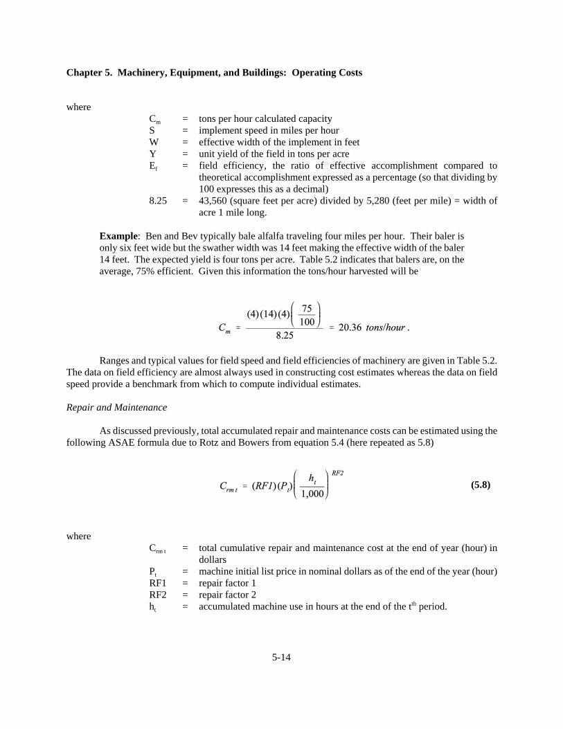
whereCm = tons per hour calculated capacityS = implement speed in miles per hourW = effective width of the implement in feetY = unit yield of the field in tons per acreEf = field efficiency, the ratio of effective accomplishment compared to

theoretical accomplishment expressed as a percentage (so that dividing by100 expresses this as a decimal)

8.25 = 43,560 (square feet per acre) divided by 5,280 (feet per mile) = width ofacre 1 mile long.

Example: Ben and Bev typically bale alfalfa traveling four miles per hour. Their baler isonly six feet wide but the swather width was 14 feet making the effective width of the baler14 feet. The expected yield is four tons per acre. Table 5.2 indicates that balers are, on theaverage, 75% efficient. Given this information the tons/hour harvested will be

Ranges and typical values for field speed and field efficiencies of machinery are given in Table 5.2.The data on field efficiency are almost always used in constructing cost estimates whereas the data on fieldspeed provide a benchmark from which to compute individual estimates.

Repair and Maintenance

As discussed previously, total accumulated repair and maintenance costs can be estimated using thefollowing ASAE formula due to Rotz and Bowers from equation 5.4 (here repeated as 5.8)

whereCrm t = total cumulative repair and maintenance cost at the end of year (hour) in

dollarsPt = machine initial list price in nominal dollars as of the end of the year (hour)RF1 = repair factor 1RF2 = repair factor 2ht = accumulated machine use in hours at the end of the tth period.


5-15

(5.9)

For repairs and other costs estimated as a function of price, the initial list price in nominal dollarsat the end of the current period is used. The initial list price is more stable than purchase price because ofperiodic dealer discounts and marketing incentives. It is assumed that the cumulative repair cost formula doesnot include any interest on the expense. For costs like depreciation (capital recovery), the expectedpurchase price after including typical discounts and incentives, rather than the list price, is used.

Example: Ben and Bev Dairyman own a 140-horsepower two-wheel (2WD) drive tractorand a 8-row (narrow) planter. These two machines will be used to illustrate estimating repaircosts. For the purposes of this example we assume the tractor's initial list price is $58,971.If there is no inflation, this would give a value in current nominal dollars of $58,971. Withinflation of 4.0% per year, the year-end value would be $61,329.84. And we assume thatBen and Bev plan to use the tractor 300 hours per year and own the tractor for 20 years, atotal of 6,000 hours of use. From Table 5.2, the repair cost factors are RF1 = .007 and RF2= 2.0. The total repair costs over the period the tractor is owned are computed as follows:

The total repair cost assuming 4% inflation for this year would be $15,455.12. Figure 5.2shows the total accumulated repairs for 2WD tractors with 500 hours of annual use as theyare used. Repair cost is expressed as a percent of list price.

The planter has a list price of $18,095 and will be used 75 hours per year for 15 years, a totalof 1,125 hours. From Table 5.2, the repair factors are RF1 = .32 and RF2 = 2.1 so the costis as follows:

Equation 5.8 gives total accumulated repair and maintenance costs for a machine that has been usedht hours. The average cost per hour is calculated as

whereR/MCOSTh = average repair and maintenance cost per hourht = accumulated use of the machine in hours at the end of year tCrmt = total cumulative repair and maintenance cost in dollars.


5-16

Figure 5.2. Total Accumulated Repairs as a Function of Hours of Use

Example: The total accumulated repair and maintenance cost of $14,860.69 for the tractorover the 6,000 hours the tractor is expected to be owned gives an expected hourly tractorrepair charge of $2.4767. This gives an annual expense, assuming 300 hours of use, equalto $743.03. With inflation of 4.0% this is an annual cost of $772.75 and an hourly cost of$2.58. Using the same procedure, the $7,415.30 planter repair cost over 1,125 hoursconverts to an hourly expected repair charge of $6.5914 and an annual charge of $494.35.With inflation of 4% in current year this is an hourly charge of $6.86.

Time Adjustments for Repair Costs

Equation 5.8 can be used to estimate the total repair costs over the time of machine ownership. It isnormally expected that as a machine ages, annual repair costs will rise. Although dividing the total lifetimerepair costs by the number of hours of use gives the average repair per hour, it does not take into account therelative greater importance of current repair costs relative to costs later in machine life. As long as annualcosts are more or less stable throughout the life of the machine, as with fuel and lubricants, considering when


5-17

(5.10)

(5.10a)

those costs occur is not particularly important given their relatively low annual level as compared to othercosts. However, because it is expected that most repairs will occur later in machine life, it is likely that repaircosts are being overestimated when equations 5.8 and 5.9 are used directly.

An alternative procedure to assuming uniform repairs over the life of the machine is to estimate theexpected annual or hourly repair expenditure for each year of machine ownership using equation 5.8recursively. Because of the uncertain nature of repair costs, this is not a recommended procedure forestimating expected costs for a particular year. However, for determining an average repair cost reflectingdifferential time flows, this recursive procedure is appropriate. Based on equation 5.8, equation 5.10 permitsestimating the expected repair cost in any particular year (or hour). Cumulative repairs at the beginning of

the tth period in beginning-of-period dollars are given by . Repairs at the

end of the period are given by . The difference between these two is the

nominal repair cost in the tth year. But if a real repair cost is being estimated, the same price must be used foreach term as follows:

whereRCt = repair costs for year t in dollarsPt = machine list price in nominal dollars at the end of year t RF1 = repair factor 1RF2 = repair factor 2ht-1 = accumulated machine use at beginning of year (or hour) t in hoursht = accumulated machine use at end of year (or hour) t in hours.

The second term in the first line of 5.10 is the cost in current dollars of the cumulative repairs as of the endof the previous period. It is based on the list price of the machine at the end of the current period but withusage as of the beginning of the period. When Pt is constant over time, equation 5.10 can be written (using5.8) as follows:


5-18

Example: Consider the 140-horsepower 2WD tractor owned by Ben and Bev Dairyman.The tractor's initial list price is $58,971. The repair and maintenance factors are RF1 = .007and RF2 = 2.0. Previously the total repair cost for the 6,000 hours of useful life over 20years were computed as $14,860.69. The cumulative repair costs assuming constant pricesfor the machine over a 19-year life at 300 hours per year are computed as follows:

The costs for the twentieth year are then given by the difference between $14,860.69 and$13,411.77, or $1,448.92. Notice that because prices do not change we can simply subtractCrm19 from Crm20 to obtain the cost for year 20. If prices are changing, it is necessary to usethe first line of equation 5.10 directly or multiply Crm19 by the inflation rate so that the sameprice can be factored out in equation 5.10. The costs for other years can be computed in asimilar fashion, as in Table 5.3. One could also create a similar table with a row for eachhour or month of machine use.

T abl e 5 .3 An n u al i z e d Re pair C os t for Exam pl e T ractorT ract or Lis t p rice 58971U sefu l Life 20A nnual U se 300T ot al U s e 6000

R F 1 0.007R F 2 2R eal in t eres t 0 .05A nnual Inflat ion (if ap p licab le) 0 .04Lifet im e rep airs (no in flat ion) 14860 .69

C um m ulat ed R ep air C os t C os t in Year j C os t in Year j A nnuit yYear Inflat ion rat e 1+ r H ours H ours C os t D uring D isc. t o D isc. t o w it h Value D iscoun t ed

(act ual) B eg End at End o f Year j y ear j B eg Year 1 End Year 1 of P V0 A nnuit y1 0.000 1.050 1 .000 0 300 37.151730 37.152 35.3826 37.151730 624.369383 594.6375082 0.000 1.050 1 .000 300 600 148.606920 111.455 101.0931429 106.147800 624.369383 566.3214363 0.000 1.050 1 .000 600 900 334.365570 185.759 160.4653061 168.488571 624.369383 539.3537484 0.000 1.050 1 .000 900 1200 594.427680 260.062 213.9537415 224.651429 624.369383 513.6702375 0.000 1.050 1 .000 1200 1500 928.793250 334.366 261.9841733 275.083382 624.369383 489.2097496 0.000 1.050 1 .000 1500 1800 1337.462280 408.669 304.9551223 320.202878 624.369383 465.9140477 0.000 1.050 1 .000 1800 2100 1820.434770 482.972 343.2395316 360.401508 624.369383 443.7276648 0.000 1.050 1 .000 2100 2400 2377.710720 557.276 377.1862985 396.045613 624.369383 422.5977759 0.000 1.050 1 .000 2400 2700 3009.290130 631.579 407.121719 427.477805 624.369383 402.474071

10 0.000 1.050 1 .000 2700 3000 3715.173000 705.883 433.3508493 455.018392 624.369383 383.30863911 0.000 1.050 1 .000 3000 3300 4495.359330 780.186 456.1587888 478.966728 624.369383 365.05584712 0.000 1.050 1 .000 3300 3600 5349.849120 854.490 475.8118885 499.602483 624.369383 347.67223513 0.000 1.050 1 .000 3600 3900 6278.642370 928.793 492.5588908 517.186835 624.369383 331.11641414 0.000 1.050 1 .000 3900 4200 7281.739080 1003.097 506.632002 531.963602 624.369383 315.34896615 0.000 1.050 1 .000 4200 4500 8359.139250 1077.400 518.2479033 544.160298 624.369383 300.33234916 0.000 1.050 1 .000 4500 4800 9510.842880 1151.704 527.6087028 553.989138 624.369383 286.03080817 0.000 1.050 1 .000 4800 5100 10736.849970 1226.007 534.9028324 561.647974 624.369383 272.41029418 0.000 1.050 1 .000 5100 5400 12037.160520 1300.311 540.3058913 567.321186 624.369383 259.43837519 0.000 1.050 1 .000 5400 5700 13411.774530 1374.614 543.9814415 571.180514 624.369383 247.08416720 0.000 1.050 1 .000 5700 6000 14860.692000 1448.917 546.081756 573.385844 624.369383 235.318254

Sum 14860.692P res ent Value at B eginning o f 1 7781.022582 7781 .02258P res ent Value at End of 1 8170.073711

U S0(r,20) 12 .46221034R eal A nnuit y w ith Value P V 0 624.369383R eal A nnuit y w it h Value P V 1 655 .5878521

1


5-20

(5.11)

Because prices are assumed to be constant, the cost per year is just the difference in the cumulativecosts. For example, the cost in year 4 is 594.43 - 334.37 = $260.06. As suggested in Chapter 2, these varyingannual costs can be converted to a constant real annuity using capital budgeting procedures. The presentvalue of this cost stream at the beginning of the first year is $7,781.02. The amortized average annual repaircost with this same present value can be determined using equation 5.11 (assuming a zero inflation rate).

whereARC = amortized average annual repair costr = real interest raten = years of lifeRCj = repair costs for year j as estimated using equation 5.10US0(r,n) = uniform series having interest rate r and n periods.

This annuity can also be obtained using the standard annuity functions available on business calculators orin spreadsheet programs (such as PMT in EXCEL). Those using calculators and spreadsheet functions todetermine the present value of a series should be sure the calculations are performed assuming payments aremade at the end of each period. For the example tractor these computations are presented explicitly in Table5.3. For this example the annual repair amount is $624.37 as compared to $743.03 ($772.75 with inflation)using equation 5.8 directly and dividing the cost by total years of use. This is a payment at the end of eachyear that has the same present value as the various RCt. This annual annuity amount can then be divided bythe number of hours of use per year to estimate a repair and maintenance cost per hour. Because the annuityrepresents a payment at the end of year and repairs occur at various times during the year, these hourlyexpenses should be charged interest at a real rate from the time of occurrence to the end of the year. Usingthe real rate is appropriate because prices are assumed not to change during the year. Walker and Kletkeindicate that for a cotton budget in southwest Oklahoma, changing the repair computation procedure fromequations 5.8 and 5.9 to equations 5.11 and 5.9 for all machines can decrease the cost per acre from $19.53to $17.98 per acre. As discussed in Appendix 2C, this annuity could be combined with the annuityconstructed to represent the other costs of owning and using machinery to estimate an annual user cost of thecapital asset (Burt 1992).

A concern with repair cost estimation is whether the repair cost equations generate costs in real ornominal terms. The preceding example assumes no inflation so that nominal and real values and interest ratesare the same. If it is likely that the repair cost coefficients were estimated using survey data and were notadjusted, then the costs are likely in nominal terms. If the cost coefficients were determined by an “expert”using personal knowledge and information about the number of moving parts, and so forth, then the costs arelikely in real terms. Although it is uncertain whether the repair costs are in real or nominal terms, it is usuallyassumed that they are in real terms at the point of estimation. This means that they are assumed to be in bothreal and nominal terms as of the end of the current year (period). If the list price is in nominal terms at the


5-21

(5.12)

beginning of the production period, it should be adjusted to the end of the year using the current inflation ratebefore proceeding with repair cost estimation. Each of the costs in subsequent years can then be adjusted tothe beginning of the first period to obtain a present value of total accumulated repair and maintenance costs.This present value can then be converted to an annuity for use in projecting average annual costs. Theconvention is to compute a real annuity having the same present value as the actual repair stream (real ornominal) and then adjust it using the appropriate inflation rate to obtain a nominal (or real) cost for each year.

It is usually assumed that repair costs occur and are paid when the machine is used. These costs willaccumulate operating interest on repair and maintenance costs from the time the operation takes place untilthe end of the estimation period. The computed real annuity after inflation adjustments (or annual repair costusing equation 5.8) is in nominal terms at the end of the first period (year). Expenditures for repairs prior tothe end of the period will accrue interest at a nominal rate from the point of occurrence to the terminationpoint. But because inflation is assumed to occur during the production period, the actual expenditure at theearlier point has a lesser nominal value. Specifically, if ae is a nominal payment at the end of the period, then

the value at an expenditure point k months earlier is where B is the annual inflation rate.

If this expenditure accrues interest at a nominal rate (i) the total cost including interest is given by

To compute the interest component we subtract the expenditure without interest and then simplify,

where ic(repairs) is the interest charge. This is the nominal interest on the nominal expenditure ( )

for k months as given by equation 2.15.

Total repairs for a year in nominal dollars are usually allocated over the year by hours using totalhours of use per year as in equation 5.9. This gives a cost per hour of use in end-of-year dollars. If hours ofuse per month are equal, this annual total cost can be divided into a nominal cost per month by finding aconstant real cost per month that translates into total nominal expenditure. If real and nominal prices andcosts are equal as of December 31 then a constant real cost, ar, can be found using equation 5.13,


5-22

(5.13)

(5.14)

(5.15)

where the sum of nominal costs adds up to nominal expenditures (Nom Exp). Standard annuity functions andequation 5.14 can be used to find ar,

where Bm is the monthly inflation rate computed from equation 2.12. The last expression is obtained using

equation 2B.7 and is the annuity having a present value of Nom Exp multiplied by . This

expression is thus easy to compute using standard functions such as PMT in Excel. By multiplying ar by theappropriate monthly discount factor, a nominal cost per month for repairs is found. In such a nominalanalysis with prices rising at the rate of inflation during the year, an hour of machine time will cost less atthe beginning of the year than at the end. The nominal cost at the end of the year is the sum of the costs eachhour or month.

If, as is probably more common, the number of hours per month varies over the year, a morecomplicated procedure is needed. In such a situation it is appropriate to find a constant real price per hourwhich, when adjusted for inflation and then multiplied by the number of hours per month and summed, isequal to total nominal expenditures. If the base period is the end of the twelfth month (December), we seeka constant real repair cost per hour R/Mh such that the following identity holds:

where it is assumed that R/Mh is the real and nominal cost per hour at the end of December and hj is hoursof use in the jth month (1=January and so forth). This equation can be solved for R/Mh as in equation 5.14 asfollows:


5-23

(5.16)

(5.17)

Unlike equation 5.14, this cannot be simplified using standard annuity formulas due to the presence of hj inthe summation. This real value can then be adjusted for inflation to give a nominal cost per hour for eachmonth. This nominal cost per hour is given by

where the superscript n denotes the nominal cost and j denotes the jth month.

Given the complexity of equations 5.14 and 5.16, an alternative is to assume constant nominalexpenditures over the course of the year and use the average nominal cost per hour in year-end dollars as thecost for all hours during the year. This nominal cost per hour at the end of the year is also the real cost perhour since real and nominal values are equal at the end of the period. These “average” expenditures will, ofcourse, sum to the total, but will overstate costs in the first part of the year.

Example: Consider the example tractor with an assumed list price $58,971 and an annualinflation rate during the first year of 4.0%. This gives a year-end nominal list price of$61,329.84. The total accumulated repair and maintenance cost of $15,455.12 for the tractorover the 6,000 hours the tractor is expected to be owned gives an expected hourly tractorrepair charge of $2.5785 which is reported in the cost per hour column in the exhibit belowon the line labeled Nominal repair cost (equal use per month). This gives an annual expense,assuming 300 hours of use, equal to $772.756. The operating interest on this can becalculated in a variety of different ways. Exhibit 5.1 below shows the computations for threealternative methods.


5-24

Exhibit 5.1 Alternative Methods to Calculate Interest on Repair Expenses

List price of tractor 58971Useful life of tractor 20Annual use 300Total use 6000RF1 0.007RF2 2Real interest rate 0.05Inflation rate 0.04Nominal interest rate 0.092M onthly inflation rate 0.003274Total repair expense over tractor's life (inflation = 4%) 15455.12Cost/hour for repairs 2.575853Cost/year for repairs 772.756US0 (monthly inflation, 12) 11.7485

Cost 1 2 3 4 5 6 7 8 9 10 11 12 Per Per Item Per Hour Jan Feb M ar Apr M ay Jun July Aug Sep Oct Nov Dec M onth YearHours of use per month 15.00 20.00 20.00 30.00 45.00 30.00 25.00 25.00 30.00 30.00 20.00 10.00 25.000 300.000

Real repair cost (equal use per month) 2.62241 65.56 65.56 65.56 65.56 65.56 65.56 65.56 65.56 65.56 65.56 65.56 65.56 65.560Nominal repair cost (equal use per month) 2.57585 63.25 63.45 63.66 63.87 64.08 64.29 64.50 64.71 64.92 65.13 65.35 65.56 64.396 772.756Interest on line above 5.31 4.83 4.34 3.86 3.38 2.89 2.41 1.93 1.44 0.96 0.48 0.00 31.837

Nominal repair cost (average cost/hour & actual use) 2.57585 38.64 51.52 51.52 77.28 115.91 77.28 64.40 64.40 77.28 77.28 51.52 25.76 64.396 772.756Interest on line above 3.25 3.92 3.52 4.67 6.11 3.48 2.41 1.92 1.72 1.14 0.38 0.00 32.497

The first line gives the actual hours of use each month. If this information were not availableand it was instead assumed that hours of use per month were equal, equation 5.14 could beused to obtain a constant real payment that when converted to nominal terms would sum tothe annual total expense of $772.756. The computations are as follows:

This real payment appears in the per month column (and also the other columns) on the Realrepair cost (equal use per month) line of Exhibit 5.1. The cost per hour in the real repair costline is given by dividing the cost per month by the hours per month ($65.5602/25) to obtain$2.6224. This amount can then be adjusted to a nominal basis using the monthly adjustmentformula analogous to equation 5.17. For example, the nominal cost in the eighth month[R/Mn (8)] is given by

The sum of these costs is $772.756. Note that the cost per hour in effect rises over the yearso that the cost of 25 hours in January is less than in December. Nominal interest on theseexpenses is $31.837.


5-25

(5.18)

Rather than assuming that repairs are evenly spaced over the year, we can use the nominalcost per hour and multiply it by the hours of use each month. This will give the correct totalrepairs but will not allocate them in a way that accounts for rising prices during the year. Toobtain the cost in the eighth month, take the number of hours in the eighth month (25) andmultiply by the average cost per hour ($2.5758) to obtain $64.395. In this case, the costs inJune and September are the same since the hours are the same. Nominal interest in this caseis $32.497.

The final and correct method is to construct a nominal cost per hour that is different for eachmonth, accounts for different use per month, and sums to total nominal cost. This is doneusing equations 5.16 and 5.17. The denominator of equation 5.16 is constructed in the lineof Exhibit 5.1 labeled Inflation-adjusted hours. The sum of this row is the denominator of5.16. The real cost per hour is then given by

This is reported in the cost/hour column and the real repair cost (actual use) line. Thenominal cost per hour can be calculated for each month using 5.17. For the eighth monthwe obtain

The sum of these expenditures is also $772.756. This set of monthly expenditures allowsfor differential hours and prices (due to inflation) each month. The interest on theseexpenditures is $32.322. This is less than the interest expense computed using the averagenominal cost per hour for every month and will always be so if inflation is positive.

Given the fact that interest on repair expenditures is usually a small proportion of total costs, the errorcreated by charging interest on the average rather than the correct nominal value is probably not significant.In situations where computations are completely automated using a computer program, the cost of using thecorrect procedure is not great and could be used.

If it is assumed that all repair costs are estimated in nominal dollars, then equation 5.18 can be usedto estimate a real amortized average annual repair cost. The primary difference is that each repair cost mustbe additionally deflated by the inflation rate to convert it to real dollars.

whereARC = amortized average annual repair cost


5-26

(5.10b)

Bj = inflation rater = real interest raten = years of lifeRCj = repair costs for year j as estimated using equation 5.10 assuming all costs

are in nominal dollars.

Equation 5.18 is a general form of 5.11 and will yield the same answer when inflation is zero in every period.If we assume that inflation occurs each year at a 4.0% rate, then nominal machine repair cost will increaseover time as in Table 5.4. The cost during year t is computed by subtracting from the accumulated cost atthe end of year t [RCt], the inflation-adjusted cost at the end of year t-1 [(1+B)RCt-1 ]. This is made precisein equation 5.10b where Bt is the inflation rate in period t.

Table 5.4 Annualized Repair Cost for Example Tractor with 4% Inflation Each YearTractor List p rice 58971Useful Life 20Annual Use 300Total Use 6000

RF1 0.007RF2 2Real interest 0.05Annual Inflation (if app licable) 0.04Lifetime rep airs (no inflation) 14860.69

Cummulated Repair Cost Cost in Year j Cost in Year j AnnuityYear Inflation rate 1+r Hours Hours Cost During Disc. to Disc. to with Value Discounted

(actual) Beg End at End of Year j y ear j Beg Year 1 End Year 1 of PV0 Annuity1 0.040 1.050 1.040 0 300 38.63779920 38.63780 35.3826 38.6377992 649.34416 594.637512 0.040 1.050 1.040 300 600 160.73324467 120.54993 101.0931429 110.393712 675.31792 566.321443 0.040 1.050 1.040 600 900 376.11579253 208.95322 160.4653061 175.2281143 702.33064 539.353754 0.040 1.050 1.040 900 1200 695.39630975 304.23589 213.9537415 233.6374857 730.42387 513.670245 0.040 1.050 1.040 1200 1500 1130.01900334 406.80684 261.9841733 286.0867172 759.64082 489.209756 0.040 1.050 1.040 1500 1800 1692.31645941 517.09670 304.9551223 333.0109936 790.02645 465.914057 0.040 1.050 1.040 1800 2100 2395.56796587 635.55885 343.2395316 374.8175685 821.62751 443.727668 0.040 1.050 1.040 2100 2400 3254.06130221 762.67062 377.1862985 411.8874379 854.49261 422.597779 0.040 1.050 1.040 2400 2700 4283.15818903 898.93443 407.121719 444.5769171 888.67232 402.47407

10 0.040 1.050 1.040 2700 3000 5499.36360073 1044.87908 433.3508493 473.2191275 924.21921 383.3086411 0.040 1.050 1.040 3000 3300 6920.39915516 1201.06101 456.1587888 498.1253973 961.18798 365.0558512 0.040 1.050 1.040 3300 3600 8565.28080560 1368.06568 475.8118885 519.5865823 999.6355 347.6722413 0.040 1.050 1.040 3600 3900 10454.40107216 1546.50903 492.5588908 537.8743088 1039.6209 331.1164114 0.040 1.050 1.040 3900 4200 12609.61606242 1737.03895 506.632002 553.2421462 1081.2058 315.3489715 0.040 1.050 1.040 4200 4500 15054.33754392 1940.33684 518.2479033 565.9267104 1124.454 300.3323516 0.040 1.050 1.040 4500 4800 17813.63034530 2157.11930 527.6087028 576.1487035 1169.4321 286.0308117 0.040 1.050 1.040 4800 5100 20914.31537728 2388.13982 534.9028324 584.1138929 1216.2094 272.4102918 0.040 1.050 1.040 5100 5400 24385.07857968 2634.19059 540.3058913 590.0140333 1264.8578 259.4383719 0.040 1.050 1.040 5400 5700 28256.58611714 2896.10439 543.9814415 594.0277342 1315.4521 247.0841720 0.040 1.050 1.040 5700 6000 32561.60616269 3174.75660 546.081756 596.3212775 1368.0702 235.31825

Sum 25981.646Present Value Beginning of 1 7781.022582 7781.0226Present Value End of 1 8496.876659

US0(r,20) 12.46221034Real Annuity PV 0 624.369383Real Annuity PV 1 681.8113662

1 1


5-28

Equation 5.10b is equivalent to equations 5.10a and 5.10 when the inflation rate is zero. The cost in year 4in Table 5.4 is obtained as 695.3963 - (1.04)( 376.1158) = $304.2359. The present value of this entire incomestream is $7,781.023, as before. The inflation-adjusted annuity value of $649.34 would be used as the costfor the first year. This could then be divided by the hours of use per year to get a cost per hour. This wouldthen be charged interest at the nominal rate for the year from the time the hour of machine time was consumeduntil the end of the period.

If, as suggested in Chapter 2 and discussed in more detail in Chapters 6 and 10, nominal interest rates(including inflation) are assumed for the current year but real rates are used for periods other than the currentone, equation 5.18 can be adjusted to reflect no inflation in list prices past the first year and then use realinterest rates for future periods. If inflation occurs at a 4.0% rate during the production year but it is assumedthere is no inflation thereafter, the results in Table 5.5 are obtained. As before, the present value of the coststream is $7,781.023 with a real annuity value of $624.369. It is increased in the first year by 4.0% to$649.344 and remains the same thereafter. This can then be divided by annual hours of use to obtain a costper hour. Interest on repair costs during the year occur at a real rate of interest.

The Task Force recommends that repair costs be estimated using either equations 5.8 and5.9, which do not adjust for repair costs changing over time, or equations 5.18 and 5.9,which create a constant real annuity that reflects changing costs over time. If the latterset of equations (based on capital budgeting) are used to estimate repair costs, it isimportant these equations also be used for depreciation, taxes, and other costs that mayvary substantially through time.

Repair Cost Estimates for Used Machines

It is expected that as machines age, repairs per hour will increase. This is also one of thecharacteristics of the repair cost equations. Thus repairs for a portion of machine life beginning at some pointafter the machine is new can be estimated by first determining repairs for the number of hours of use beforeacquisition and subtracting the results from the expected repairs for total machine life at the time it is retiredby the second owner. Repair costs vary widely and the results are good only for use as expected repairs. Asmachines age, overhauls will be required and whether that occurs before or after a used machine is purchasedcan affect repair costs significantly.

Example: One of the tractors on the Midwest Dairy Farm was purchased used. A 1982140-horsepower tractor was purchased in 1987 and had been used for 2,750 hours as of thebeginning of 1992. The real list price of this tractor as of the end of 1991 is estimated to be$58,971 based on the list price of a similar new tractor in 1991. The Dairymans expect touse the tractor for 10 additional years for about 300 hours each year. When Ben and Bev sellthe tractor, it will have a total of 5,750 hours (2,750 + (10)(300)) of use. We compute thecumulative cost of repairs over the first 10 years of use and then the cost of repairs over thesecond 10 years of use. This will give a higher cost per hour for the second ten years giventhe rising pattern of repair costs.

Table 5.5 Annualized Repair Cost for Example Tractor with 4% Inflation in Production Year and None ThereafterTractor List price 58971Useful Life 20Annual Use 300Total Use 6000

RF1 0.007RF2 2Real interest 0.05Annual Inflation (if applicable) 0.04Lifetime repairs (no inflation) 14860.69

Cummulated Repair Cost Cost in Year j Cost in Year j AnnuityYear Inflation rate 1+r Hours Hours Cost During Disc. to Disc. to with Value Discounted

(actual) Beg End at End of Year j year j Beg Year 1 End Year 1 of PV0 Annuity1 0.040 1.050 1.040 0 300 38.63779920 38.63780 35.3826 38.6377992 649.34416 594.637512 0.000 1.050 1.000 300 600 154.55119680 115.91340 101.0931429 110.393712 649.34416 566.321443 0.000 1.050 1.000 600 900 347.74019280 193.18900 160.4653061 175.2281143 649.34416 539.353754 0.000 1.050 1.000 900 1200 618.20478720 270.46459 213.9537415 233.6374857 649.34416 513.670245 0.000 1.050 1.000 1200 1500 965.94498000 347.74019 261.9841733 286.0867172 649.34416 489.209756 0.000 1.050 1.000 1500 1800 1390.96077120 425.01579 304.9551223 333.0109936 649.34416 465.914057 0.000 1.050 1.000 1800 2100 1893.25216080 502.29139 343.2395316 374.8175685 649.34416 443.727668 0.000 1.050 1.000 2100 2400 2472.81914880 579.56699 377.1862985 411.8874379 649.34416 422.597779 0.000 1.050 1.000 2400 2700 3129.66173520 656.84259 407.121719 444.5769171 649.34416 402.47407

10 0.000 1.050 1.000 2700 3000 3863.77992000 734.11818 433.3508493 473.2191275 649.34416 383.3086411 0.000 1.050 1.000 3000 3300 4675.17370320 811.39378 456.1587888 498.1253973 649.34416 365.0558512 0.000 1.050 1.000 3300 3600 5563.84308480 888.66938 475.8118885 519.5865823 649.34416 347.6722413 0.000 1.050 1.000 3600 3900 6529.78806480 965.94498 492.5588908 537.8743088 649.34416 331.1164114 0.000 1.050 1.000 3900 4200 7573.00864320 1043.22058 506.632002 553.2421462 649.34416 315.3489715 0.000 1.050 1.000 4200 4500 8693.50482000 1120.49618 518.2479033 565.9267104 649.34416 300.3323516 0.000 1.050 1.000 4500 4800 9891.27659520 1197.77178 527.6087028 576.1487035 649.34416 286.0308117 0.000 1.050 1.000 4800 5100 11166.32396880 1275.04737 534.9028324 584.1138929 649.34416 272.4102918 0.000 1.050 1.000 5100 5400 12518.64694080 1352.32297 540.3058913 590.0140333 649.34416 259.4383719 0.000 1.050 1.000 5400 5700 13948.24551120 1429.59857 543.9814415 594.0277342 649.34416 247.0841720 0.000 1.050 1.000 5700 6000 15455.11968000 1506.87417 546.081756 596.3212775 649.34416 235.31825

Sum 15455.11968Present Value Beginning of 1 7781.022582 7781.0226Present Value End of 1 8496.876659

US0(r,20) 12.46221034Real Annuity PV 0 624.369383Real Annuity PV 1 681.8113662

1 1


5-30

(5.19)

The total repairs for hours 2,751 through 5,750 = $13,648.10 - $3,121.78 = $10,526.32. Thisgives a cost per hour for the remainder of the life of the machine of $3.51 (10,526.32/3,000).If there was 45 inflation during the current year, this would be revised to $14,194.02 -$3,246.65 = $10,947.37 or $3.649 per hour.

Fuel and Lubricants

Fuel and lube costs also can be estimated by survey or engineering equations. Survey proceduresappropriate for general machinery operating costs also can be appropriate for fuel and lubricants. ASAEequations can be used to estimate the fuel efficiency or fuel consumption of the power unit. The fuelconsumption is then multiplied by the fuel cost per unit to estimate fuel cost. Oil consumption can beestimated using engineering equations as well.

Engineering Equation Fuel Cost Estimates

The ASAE Standards give two methods for estimating fuel consumption. An average method canbe used when an estimate of annual average fuel consumption for power units is all that is needed. Thismethod is useful for predicting overall machinery costs for a given enterprise. When determining the costsfor a specific operation (planting), fuel requirements should be based on the detailed formulas.

Average annual fuel consumption for a given power unit can be estimated as follows:

whereGasgph = average gasoline consumption, gallons per hourDieselgph = average diesel consumption, gallons per hourLPGgph = average liquefied petroleum consumption, gallons per hourPTOmax = maximum PTO horsepower per hour.


5-31

(5.20)

(5.21)

The detailed method for estimating fuel consumption per hour is calculated as

whereFgph = fuel consumption in gallons per hourHPR = equivalent PTO horsepower requiredFMfuel = fuel use multiplier for fuel type as defined below.

The fuel multipliers (FM) are given in equation 5.21.

whereFMgas = fuel multiplier for gas engines, gallons per horsepower per hourFMdiesel = fuel multiplier for diesel engines, gallons per horsepower per hourFMlpg = fuel multiplier for lpg engines, gallons per horsepower per hourHPR = equivalent PTO horsepower requiredHPM = maximum PTO horsepower.

Example: The more detailed way to estimate fuel consumption is with equations 5.20 and5.21. The additional information required is the equivalent HPR required to pull the load forthe implement in question. For this illustration it is assumed that the planter requires using70 of the 140 horsepower available.


5-32

(5.22)

Engineering Equation Lube Cost Estimates

A general estimate of oil consumption given by the ASAE Standards is .01 to .025 gallons per hour,depending on the volume of the engine crankcase. A detailed method relating oil consumption to engine sizeis given by the ASAE Standards as

whereOilgas = oil consumption for gas engines, gallons per hourOildiesel = oil consumption for diesel engines, gallons per hourOillpg = oil consumption for lpg engines, gallons per hourHP = rated engine horsepower.

Example: The estimated lube cost for the tractor is

If filters are changed every other oil change, the total lube cost per hour approaches 15% of the total fuel cost.

Suggestions for Estimating Costs for Machines Not Listed in Tables

It is impossible for Table 5.2 to include all machines. When costs must be estimated for a machinenot listed, and cost estimates are not otherwise available, it is suggested that parameters for a similar machinebe used. Look through the tables for a machine having a similar number of moving parts, a similar powersource, and a similar type of use. When estimating repairs, the key parameter in Table 5.2 is the ASAE totallife repair cost. This coefficient determines the dollar amount of repairs over machine life. The otherparameters only determine the distribution of those costs over machine life. For any machine, the equationsprovide an estimate of expected average repair costs over a number of hours of use and it is not likely thatusing coefficients for a similar machine will greatly over- or underestimate expected repair costs.

IRRIGATION OPERATING COSTS

There is not a consensus for how to estimate repair costs for irrigation equipment. The ASAE doesnot publish equations for estimating repair costs of irrigation equipment in the ASAE Standards, andextensive surveys have not been undertaken to estimate these costs.


5-33

Example Irrigation System

System Component Initial Cost

Well (250 feet) $11,850Column Pipe (200 feet) $8,016Electric Switches $1,701Electric Service $4,976Land Shaping $4,000Pump Base $1,433Pump $3,335Electric Motor $3,190Sprinkler System $30,000 Total $68,501

One of the key elements in determining irrigation costs is application efficiency. For example, if theintent is to apply 12 inches of water using a surface system and if the application efficiency of floodapplication is 60%, it will be necessary to pump 20 inches of water to obtain the desired 12 inches. Theapplication efficiency depends on the type of irrigation system, the type of soil, and weather conditions suchas wind velocity and humidity.

Repair and Maintenance Cost Estimates

Jensen [1980] gives guidelines on estimating annual maintenance and repairs as a percent of initialcost. McGrann et al. [1986a, 1986b] use these same procedures. Table 5.6 gives these estimates for typicalirrigation equipment. Thompson and Fischbach and later Selley use a different approach to estimating repairand maintenance costs for irrigation equipment. Table 5.7 gives the estimated repair and maintenance costfor power units and Table 5.8 presents delivery system repair and maintenance. As an example consider thefollowing system.

Repair estimates using the McGrann et al. procedure are determined by applying coefficients from Table 5.6to the expected investment given above. The McGrann et al. procedure provides annual estimates that do notdepend on use. In this illustration the average of the upper and lower percent range in costs is used.


5-34

Repair Costs - McGrann et al. Procedure

Item Percent Annual Cost

Well 1 $118.50

Column Pipe 4 $320.64

Electric Switches 2 $34.02

Electric Service 0 0.00

Land Shaping 0 0.00

Pump Base 1 $14.33

Pump 6 $200.10

Electric Motor 2 $63.80

Sprinkler System 6.5 $1,950.00

Total Annual Repairs $2,701.39


5-35

Repair Costs - Selley Procedure

Item Rate Hourly CostPower Unit $.62/bhp/1,000 hr $0.05

20 hrs labor/1,000 hr@ $15/hr $0.30

Delivery System ($0.08) (Pivot length/125) $0.83 Total/Hour $1.18

(5.23)

Repair cost estimates using the Selley procedure are given next. Repairs and maintenance areestimated on an hourly basis using the coefficients found in Table 5.7.

Assuming an annual use of 1,000 hours per year, the McGrann et al. procedure yields an estimate of $2.70per hour, more than two times the estimate of Selley. Even if the lower end of the repair cost range fromTable 5.6 is used, the McGrann et al. procedure yields an annual estimate of $2.05 per hour for the system,still significantly higher than the Selley method.

Energy Cost Estimates

McGrann et al. use the following procedure to estimate energy costs.

whereWHP = water horse powerGPM = gallons per minute pumped from wellFEET = static water depthPSI = system pressure, in pounds per square inchTBHP = brake horse power


5-36

PE = pump efficiencyGDE = gear drive efficiency (equals 1 for non-turbine)PHRS = engineering estimate of annual useACIN = total acre inches pumpedTFU = annual fuel useBTU = BTU's per unit of fuelEE = engine efficiencyFC = total fuel costFCOST = cost per unit of fuel.

Table 5.9 gives the efficiency of irrigation components and Table 5.10 gives the BTU energy for thetypical fuel alternatives. The energy cost estimates for the McGrann et al. procedure follow. The system isa low pressure center pivot system (800 gallons/minute, 35 PSI, 130 acres, 250N well, 200N column, 125N lift,and 206N head). The pump is driven by a 75 bhp electric motor and electricity is $0.08 per KWH. Costs areestimated for one hour of use.

Energy Cost for Center Pivot Irrigation SystemMcGrann et al. Procedure

The water horsepower required for the system is 41.58. This converts to a brake horsepower requirement of64.39. Because this is less than the 75 brake horsepower engine specified, the engine size is adequate.Because the goal is to estimate costs for one hour, the acre inches, 1.77, are chosen so that the hours requiredequals 1.00. The hourly energy use is 64.39 KWH, which costs $5.15 per hour.

Thompson and Fischbach and Selley estimate energy consumption for irrigating from the water horsepower (WHP) requirement of the irrigation system. The WHP is estimated for all system types except centerpivot as follows.


5-37

(5.24)

(5.25)

(5.26)

whereWHP = water horse powerHead = lift + (system pressure) (2.31)GPM = gallons per minute system delivery.

For center pivots, WHP is estimated as

whereWHP = water horse powerHead = lift + (system pressure) (2.31)GPM = gallons per minute system deliveryPL = pivot length in feet.

Energy consumption is estimated as

whereEC = energy consumed per hour of operation, (gallons, kwh, or mcf depending

on energy source)WHP = water horse powerEM = energy use multiplier for energy type.

The energy use multipliers for each type are the following:


5-38

(5.27)

(5.28)

(5.29)

whereEMdiesel = energy multiplier for diesel engines, gallonsEMelectric = energy multiplier for electric motors, kwhEMlpg = energy multiplier for lpg engines, gallonsEMnatural gas = energy multiplier for natural gas engines, mcfEMgasoline = energy multiplier for gasoline engines, gallons.

Energy costs can be estimated by taking the energy consumption per hour and multiplying this bythe per unit energy cost. This can then be annualized by taking the per hour cost and multiplying by theannual hours the irrigation system is used. Per acre costs can be calculated from this by dividing the annualcost by the number of acres irrigated by the irrigation system.

The per hour cost of irrigation is given by

whereE$H = energy cost per hour of system useEC = energy consumed per hour of operationFC = fuel cost per unit, (gallon, kwh, mcf).

The annual cost of irrigation is computed as

whereAE$ = annual energy cost for system useE$H = energy cost per hour of system useAH = annual hours of system use,


5-39

(5.30)

and per acre costs are given by

whereE$A = annual energy cost per acre for systemAE$ = annual energy cost for system useAcres = acres of land irrigated with system.

The energy cost estimates for the Selley procedure follow. The system is a low pressure center pivotsystem (800 gallons/minute, 35 PSI, 130 acres, 250N well, 200N column, 125N lift, and 206N head). The pumpis driven by a 75 bhp electric motor and electricity is $0.08 per KWH. Costs are estimated for one hour ofuse.

Energy Cost for Center Pivot Irrigation SystemSelley Procedure

The water horsepower required for the system is 44.71. Selley estimates energy use based on the waterhorsepower required. The water horsepower, 44.71, is divided by a fuel consumption multiplier, .885, todetermine the units of energy consumed. The fuel consumed, 50.52 KWH costs $0.08 per KWH and resultsin an energy cost of $4.04 per hour of pump use.


5-40

(5.31)

(5.32)

Irrigation Lubricant Costs

McGrann et al. do not estimate a separate lubricant cost for the irrigation system. Selley estimatesoil consumption as

whereOC = oil consumed per hour of operation, gallonsWHP = water horse powerHours = hours system is usedOPU = oil multiplier for power unitOGD = oil multiplier for the gear drive.

Appropriate coefficients for OPU and OGD are

whereOPUdiesel = oil multiplier for diesel engines, gallonsOPUelectric = oil multiplier for electric motors, gallonsOPUlpg = oil multiplier for lpg engines, gallonsOPUnatural gas = oil multiplier for natural gas engines, gallonsOPUgasoline = oil multiplier for gasoline engines, gallonsOGD = oil multiplier for the gear drive, gallons.


5-41

(5.33)

(5.34)

(5.35)

Lubrication cost can be estimated similar to energy costs. The per hour costs are given by

whereL$H = lubrication costs per hour of system useOC = oil consumed per hour of operationO$ = oil cost per gallon.

Annual lubrication costs for the system are computed by multiplying per hour costs (L$H) by annualhours of use (AH)

Per acre costs are computed as

whereL$A = lubrication costs per acreAL$ = annual lubrication cost for system useAcres = acres of land irrigated by system.

The Selley procedure is used to estimate lubricant cost using the same example as previously. The requiredwater horsepower, 44.71, is divided first by the power unit lubricant multiplier and then by the gear drivelubricant multiplier. Electric systems do not require a gear drive, thus, the second term of the equation, OC,is not used.

The gallons of lubricant is estimated at .011 gallons per hour. If lubricants cost $15.00 per gallon, thelubricant cost is $0.165 for each hour the pump is used. The combined fuel and lubricant cost for the exampleis $4.21 ($4.04 + $0.17) for each hour the pump is used.


5-42

The two methods of estimating fuel and lubricant costs differ because McGrann et al. use the totalbrake horsepower (TBHP) to estimate energy consumption whereas Selley uses water horsepower (WHP).If 56.25 WHP were used in Selley’s equations, or if 55.40 TBHP were used in McGrann et al.'s equations,the two methods would give very similar results.


5-43

TABLE 5.6 Annual Maintenance and Repairs for Irrigation Equipment

Component

AnnualMaintenanceand Repairs% of Initial

Cost Component

AnnualMaintenanceand Repairs% of Initial

Cost

Wells and casings .5 - 1.5 Pipe, asbestos - cement and PVC buried .25 - .75

Pumping plant Pipe, aluminum, gated, surface 1.5 - 2.5

Structure .5 - 1.5 Pipe, steel, waterworks class, buried .25 - .5

Pump, vertical turbine Pipe, steel, coated and lined, buried .25 - .5

Bowls 5 - 7 Pipe, steel, coated, buried .5 - .7

Column, etc. 3 - 5 Pipe, steel, coated, surface 1.5 - 2.5

Pump, centrifugal 3 - 5 Pipe, steel galvanized, surface 1 - 2

Power transmission Pipe, steel, coated and lined, surface 1 - 2

Gear head 5 - 7 Pipe, wood, buried .75 - 1.25

V-belt 5 - 7 Pipe, aluminum, sprinkler use, surface 1.5 - 2.5

Flat belt, rubber and fabric 5 - 7 Pipe, reinforced plastic mortar, buried .25 - .5

Flat belt, leather 5 - 7 Pipe, plastic, trickle, surface 1.5 - 2.5

Prime movers Sprinkler heads 5 - 8

Electric motor 1.5 - 2.5 Trickle emitters 5 - 8

Diesel engine 5 - 8 Trickle filters 6 - 9

Gasoline engine, air cooled 6 - 9 Land grading 1.5 - 2.5

Gasoline engine, water cooled 5 - 8 Reservoirs 1 - 2

Propane engine 4 - 7 Mechanical move sprinklers 5 - 8

Open farm ditches 1 - 2 Continuously moving sprinklers 5 - 8

Concrete structures .5 - 1

Source: McGrann et al.


5-44

TABLE 5.7 Repair and Maintenance Costs of Power Units

$/BHP/1,000 hrs Hrs Labor/1,000 hrs

Diesel 5.00 20

Electric .62 20

Propane, Natural Gas 2.40 40

Gasoline 3.15 40

Source: Selley.

TABLE 5.8 Delivery System Repair and Maintenance Cost Per Hour

System Type $/hr

Pivot

Gated Pipe

Side Roll

Skid Tow

Big Gun

Reuse

Source: Selley.


5-45

TABLE 5.9 Energy Use Efficiency of Irrigation Components

ItemEngine

Efficiency (%)

Electrical Engine

< 20 HP 91

> 20 HP 87

Diesel Engine 32

Natural Gas Engine 28

Gasoline Engine

Air Cooled 26

Water Cooled 26

Propane Engine 28

PumpEfficiency (%)

Centrifugal Pump 75

Turbine Pump Discharge Head 75

Gear DriveEfficiency (%)

Gear Drive

Right Angle 95.0

Direct 100.0

Belt, V-Belt 92.5

Flat Belt 87.5


5-46

TABLE 5.10 BTUs of Energy Per Unit of Fuel

Energy Source BTU Unit

Diesel 135,250 gallon

Electricity 3,410 KWH

Gasoline 124,100 gallon

LP Gas 92,140 gallon

Natural Gas 1,000,000 MCF

BUILDING AND EQUIPMENT OPERATING COSTS

Klonsky (1992) conducted a survey on data and methods used to develop enterprise budgets by landgrant universities. Only 54% of those surveyed included building costs in enterprise budgets. In general,only buildings that could be charged entirely to a specific enterprise (for example, livestock buildings) wereincluded. Buildings for equipment and/or shops were almost never included. Of those that included buildingcosts, no data were collected on the repair of these buildings. Operating costs for buildings, including repairsand maintenance, could be obtained from general producer surveys, but would probably require specializedsurveys designed to track such expenditures. Data on specialized buildings such as finishing units may beavailable from manufacturers, specialized farm record keeping systems, farm management consultants, orpracticing agricultural engineers. Doane estimates repair and maintenance of buildings at 2-3% of originalpurchase or construction cost. Construction (purchase) costs for buildings might come from surveys,appraisal guides, or records of real estate transactions. More discussion of valuing the capital costs ofbuildings and equipment is contained in Chapter 6.

Operating costs for equipment, here defined as items other than farm machinery, are also difficult toestimate. Examples of items in this category are fencing, waterers, milk coolers, feed bins, feeding systems,etc. Often, these items are considered part of overhead and might not appear directly in the CAR estimate.Engineering estimates for repair and maintenance are usually specified as a percent per year of initial list price(Kletke). Where equipment is used by multiple enterprises, the costs must be allocated to the enterprise, andif the CAR estimate is being developed on a per head basis, the costs must be further allocated. Theequipment items are so diverse that when they are estimated using surveys, they will generally be part ofoverhead. Whether building and equipment costs are estimated directly or included as part of overhead, CARestimate developers should be certain that these costs are included.

INTEREST ON OPERATING COSTS (EXPENDABLE INPUTS)

All users of CAR estimates agree that interest should be included. Some view the interest as cost offunds used. Others view interest as an adjustment of all costs to a point in time. There is also some differenceof opinion about whether the interest charge should be actual interest paid to lenders, full nominal opportunity


5-47

interest, or real opportunity interest. The amount of interest charged should be based on the purpose of theCAR estimate, the amount of capital invested, and the appropriate rate of interest. Historical CAR estimatesused for evaluating the financial position of operators may include only interest paid to lenders whereas CARestimates used to develop and compare alternative government programs should include the full opportunitycost of capital. Cost and return estimates used for short-term cash flow planning may include interestexpected to be paid to lenders whereas CAR estimates used for enterprise evaluations and comparisons shouldinclude the full opportunity cost of capital.

As discussed in Chapter 2, nominal interest should be charged on all operating costs incurred duringthe production period. In essence, the interest charge adjusts all costs to a single point in time. Costs andreturns that occur at the CAR estimate termination date should not be charged interest. If costs occur at otherthan the CAR estimate termination date, interest should be charged to adjust these costs to the terminationdate.

Developing a framework for estimating interest requires that CAR estimate developers clearly statethe use of the CAR estimate and the assumptions regarding interest charges.

Interest Rate Definitions

Financial interest: dollar amount paid to lenders for the use of funds.

Nominal opportunity interest rate: imputed interest charge reflecting nominal incomeforegone as a result of investing in the current enterprise. In the context of CAR estimates,the nominal opportunity cost is used to adjust a CAR estimate to the CAR termination date.

Real opportunity interest: imputed interest charge reflecting real income foregone as aresult of investing in the current enterprise. In the context of CAR estimates, the realopportunity cost is used to adjust a CAR estimate from the current period to other periodsand from other periods to each other.

Estimating Interest for Historical CAR Estimates

Historical CAR estimates can have two basic purposes: determining the actual cash costs of operatingan enterprise or determining the economic costs of producing a unit of the enterprise. Historical CARestimates are usually prepared by (a) the USDA Economic Research Service from surveys, and(b) universities that have records available from which to estimate the historical costs of production.

Actual cash operating interest is the financial interest charge paid to a lender. This would ideally bedetermined by survey: however, most operators do not have records that would permit precise allocation ofinterest charges to CAR estimates for a particular enterprise. In ERS cost of production estimates, whole-farm interest is allocated to the farm enterprises.

The historical CAR estimates prepared by ERS to estimate the economic costs of production use acombination of surveys and opportunity cost charges to estimate cash interest costs. The amount of operatingcapital invested in an enterprise is determined by survey and the charge for using that capital is an opportunity


5-48

charge. The imputed cost of operating capital is based on the concept that rational producers expect thecapital invested in variable production inputs to earn at least as much as funds invested in a savings accountor some other interest-bearing financial instrument with similar risk. ERS currently uses a six-monthTreasury bill rate as the opportunity interest charge (Morehart et al., Agricultural Handbook No. 671, 1992).More discussion of appropriate opportunity interest rates is contained in Chapter 2.

Estimating Interest for Projected CAR Estimates

Interest charges included in projected CAR estimates are determined by three identifiablecomponents: the amount of money invested or expended, the rate of interest, and the length of time themoney is tied up in the investment or expense. Estimating the amount of money on which interest must bepaid requires knowledge of when expenditures are made and the termination date of the enterprise for aparticular cost and return estimate. As stated in Chapter 2, the Task Force recommends that projectedCAR estimates establish the end of the production period as the reference point in time and that allexpenditures and revenues be accumulated to the end of the production period. Most CAR estimatesare currently prepared using an opportunity interest rate because estimating cash interest payments to lendersrequires knowledge of the operator's equity position.

Three alternative ways of determining the interest charge with advantages and difficulties for eachare discussed here. Determining whether to use nominal or real interest rates further complicates thealternatives considered.

Alternative 1

A nominal rate of interest is used in this alternative. The approach assumes that the operator willborrow or charge at a nominal opportunity cost for all operating capital. The advantages of this rate aresimplicity and understandability. Farm operators understand the charge and even if they do not borrow allthe funds on which the charge is made, they understand the opportunity concept being used. A difficulty isspecifying what the nominal rate should be. Alternatives include (a) a rate of interest that farm operatorsmight pay for funds; (b) a rate of interest that farmers might receive for funds if an alternative investment hadbeen chosen; and (c) a weighted average of the rate actually paid for funds on the amount actually borrowedand the rate the operator would receive on funds invested in other alternatives for funds not actuallyborrowed. The correct choice for most applications is the second one that reflects the opportunity cost ofinvested funds. The most common alternative nominal rate used, as discussed in Chapter 2, is the risk- andinflation-adjusted long-term real rate of interest.

Crop CAR estimates usually terminate at the point of first transfer of a salable product and this isnormally the time at which interest charges terminate. With crop and livestock enterprises having multipleproduction periods (alfalfa and dairy cows for example), a time point must be chosen arbitrarily to terminateinterest charges. This is usually the end of a calendar year or the end of a production cycle.

After the appropriate rate is chosen, the nominal interest charge for the jth expense Cj (incurred nj

months from the terminal point of the estimation procedure) would be calculated as


5-49

(5.36)

(5.37)

(5.38)

where i is the annual nominal interest rate. The total of all interest charges can be computed as

where m is the number of expenses on which interest is charged. In a similar fashion if an enterprise hasreturns that occur before the terminal point in the year, they should also be adjusted to this terminal pointusing the same nominal interest rate.

Alternative 2

This method computes interest based on the per period rate and the applicable proportion of theperiod. This means that if the interest rate is stated as an annual level, the rate for different subperiods willbe the proportion of the year over which the cash flow is discounted, multiplied by the annual rate.Specifically, for an expense incurred n months before the terminal date of the enterprise, the approximateinterest charge is

where nj is the number of months until the enterprise terminates. This method gives a higher interest chargethan alternative 1 because the implied subperiod interest rate is higher than the actual rate computed inalternative 1.

This procedure can be modified for several conventions common in estimated CAR interestcomputations. One convention often used is to charge interest on expenditures for a fixed period, say sixmonths, for all capital used. This implies that all nj would be equal to the chosen proportion of the year.When it is assumed that all capital is invested for a certain length of time, say six months, the interest chargecan be calculated by multiplying the total capital by 6/12 and multiplying the result by the annual interest rate.Although this approach may not be as precise as charging interest on each item for the length of time thecapital is invested, it does provide a reasonable approximation for the cost of capital. Another conventionsometimes used is to charge interest from the time of input use until a specified date other than terminationdate. For these situations nj becomes the portion of a year elapsing from the time the input is purchased untilthe chosen date.


5-50

(5.39)

(5.40)

(5.41)

Alternative 3

A procedure using both real and nominal interest rates is to use the inflation rate to inflate the expenseand income items to the chosen time period (Walker and Kletke) and then apply a real interest rate to theseexpenditures. As discussed in Appendix 2A, the appropriate adjustment for each income and expense itemis

whereCj = cost of input item j

= inflation-adjusted end of year cost for item j

Rk = revenue from output k

= inflation-adjusted end of year revenue for item k

B = rate of inflationnj , nk = months of year the capital is invested.

After all costs and revenues are adjusted for inflation, the real cost of capital is computed using a realrate of interest. For each input the real rate of opportunity interest expense should be charged on each inputfor the period of time from purchase or use until termination of the CAR estimate, as in equation 5.36.Likewise, for each revenue item, there should be an opportunity interest income from the time the incomeis received until enterprise termination. This will then give

These individual items can then be summed to obtain a net real opportunity interest expense as

For crops with a single production point, there will be no inflation or opportunity interest income onthe revenue from production as long as sales come at the end of the period. For multiple production periodcrop and livestock enterprises, the value of production income must be adjusted for inflation and then receivea real rate of opportunity interest. The net of opportunity interest income and expense would be the netinterest charge (income) for the CAR estimate. The CAR estimate termination point for multiple production


5-51

period enterprises could be either the time of physical transfer of the last salable product, the end of thecalendar year, or some other arbitrarily selected date.

Comparison of Alternatives

Variations of alternatives one and two are the most common ways of determining interest chargeson CAR estimates. The rate of interest used is nominal and might be a weighted average of financial intereston borrowed capital and opportunity interest on operator-provided capital, or it might be opportunity interestonly. Alternatives one and two use the nominal interest rate as a starting point, whereas alternative threerequires knowledge of both inflation and real interest rates. Although both alternatives one and three aretheoretically correct, alternative one is the most easily understood and is generally preferred by CAR estimatedevelopers.

The distinct advantage of alternative three is having real interest determined separately from inflation.This permits the CAR estimate developer to not include inflation as an expense. There are, however,operational difficulties with alternative three. Although conceptually correct, there are numerouscomputations required. Also, accurate specification of inflation rates and real interest rates is required.Another concern is explaining the interest charge to farm operators and other CAR estimate users. Manyusers of CAR estimates understand the nominal rate of interest when it is related to what they pay for capital,particularly when interest is being paid to a lending institution. It is difficult to explain that the nominal rateis really composed of a real interest component and inflation and that only real interest should be considered.For more discussion of interest costs see the examples in Chapter 2, Tables 2.2-2.4.

CUSTOM OPERATIONS AND CUSTOM RATES

Definition

A custom operation is defined as the joint hiring of machinery, labor, and in some cases, purchasesof materials to perform a production operation. Examples of crop operations are fertilizer application, landpreparation, seeding, spraying, cultivating, harvesting, and hauling. Typical custom livestock operations arefeed mixing, sheep shearing, and manure hauling and spreading. Custom operations could include all, none,or several of the tasks performed in the production of the product. Examples where all tasks are custominclude custom crop farming or custom feedlots for finishing cattle. The charges for custom operations arecommonly called custom rates.

Overview of Issues

Almost any task in production agriculture can be performed as a custom operation. Whether or notit is appropriate to use custom rates for CAR estimation depends on their purpose. When the intent is todetermine the full cost of production, it may not be appropriate to use a custom operation unless it is typicallyperformed by a custom operator and it is believed that the custom charge fully covers the operating andownership costs of the custom operator. When the intent of the CAR estimate is to aid in financial decisions,or enterprise selection, it may be appropriate to use typical custom rates for any or all tasks. When CAR


5-52

estimates are being prepared for individual farm decision makers, it is expected that the lowest cost alternativefor acquiring a service would be used.

There are situations where local farmers do custom work for their neighbors, receiving some non-pecuniary benefits in lieu of, or in addition to, charging only what is necessary to cover their variable costs.Using these custom rates would underestimate actual production costs. If the custom operator is aneighboring farmer who does custom work after completing his own tasks, less timely operations couldreduce output and profitability. If appropriate, yield adjustments should be made.

The size and type of farm operation determines the feasibility of using custom operators. Small crop,livestock, and dairy operations often cannot justify a large investment in agricultural machinery andequipment when both the money and the use of the capital items are limited. In these situations, it is moreeconomical for small farm operators to rely on custom operations instead of owning the equipment andperforming the activities themselves. At the same time, some small operators may have access to low costequipment that would not be suitable for a larger operator.

Larger operations may often use custom operators for specialized tasks (for example, aerial sprayingor seeding, soil fumigation, crop harvesting, or manure pit pumping and spreading) in the business.Agribusiness firms specializing in these operations are usually used by larger businesses. The customoperator may provide timeliness of operation, lower cost of investment, specialized skills, and/or uniqueequipment for the operation.

It is usually desirable for all materials used in enterprise production to be listed with the CARestimate. However, when custom operators are used for labor-intensive harvesting operations, or when theyprovide specialized services, it may be difficult to divide the custom charge into costs of materials, labor,management, and custom operator profit. Where possible, custom charges should be divided intocomponents, but when not feasible, it is permissible to include a custom charge for the complete customactivity. Listing of materials is particularly important for fertilizer, pesticides, and other cost items that maycritically affect the production level or impact the social acceptability of the enterprise.

Current Procedures

Historical CAR estimates are obtained from surveys of farm operators. Because surveys include bothoperators who have and do not have custom work performed on their operations, the CAR estimate mayinclude tasks that are part custom and part operator performed. Custom expenses in ERS CAR estimates areestimated from data reported in the Agricultural Resource Management Study (ARMS). Some states alsoperform surveys to determine costs of production.

Projected CAR estimates developed by land grant university extension and research staff, and others,are based on a composite of farm record program summaries, producer panels, cost estimation equations, andthe expectations of expert panels. In projected CAR estimates, each operation will usually be performedeither by the farm operator or a custom operator, but not a mixture of the two. If there are operations wherecustom operators are typical and where operators also perform the operation, multiple enterprise CARestimates can be developed to reflect the different practices.


5-53

Custom rates per unit of production (planted acre, breeding animal, and hundredweight of products)are estimated by dividing the total custom expense by the number of planted acres, the number of breedinganimals, or number of units of product. Where custom operations are performed by profit-oriented customoperators, custom rates can be used as a proxy for the operating and ownership costs of a specific operationor a series of operations in the enterprise.

Recommended Procedure

Custom operations should be appropriate for the intended use of the CAR estimate. When full costsof production are being estimated, custom charges can be used when it is believed that the chargeincludes the full ownership and operating costs of the operation. However, if the custom operator is notprofit motivated and the resulting custom rate does not cover operating and ownership costs, then using thecustom rate would underestimate the true cost of production. Materials and labor requirements shouldbe listed unless the custom operator cannot accurately divide the amount charged into components.It is particularly important to list amounts and types of fertilizer, pesticides, and other inputs that may affectthe production quantity or enterprise desirability.

On small farms, custom charges may be appropriate because operators can lower their costs by hiringtasks performed. (Developers of CAR estimates should be certain that the charge includes ownership andoperating costs.) On large farms, custom operations may occur because custom operators can providespecialty services in a timely fashion less costly than the operator can perform the task(s).

When ownership and operating costs for a production practice are difficult to estimate directly,custom rates might be used as a proxy to estimate the costs for a specific production input, even though theoperator might perform the task. This procedure should be avoided if at all possible, because the actual coststo the operator might be either higher or lower than the custom charge.

OTHER COMMODITY-SPECIFIC COSTS

There are numerous costs which must be dealt with on an item-by-item basis. These costs can bedivided into several groups having similar characteristics. Following is a discussion of the groups and someof the characteristics of costs in each group. This section concludes with a discussion of examples for eachcost group.

The purpose of developing generalized CAR estimates is to provide information that will be usefulfor the many alternative uses made of CAR estimates. It is essential that costs reflect the actual and full costsof performing a task or providing a service. With this in mind, costs included in this section should includeboth direct costs to the producer as well as reductions in prices received because of involuntary checkoffs ormarketing charges. Cost and return estimates should provide sufficient information so that either net returnsto producers or economic costs of production can be estimated.


5-54

General Guidelines

• If possible, cost items should not be subtracted from the commodity price. For example,transportation costs should not be subtracted from the price of the product, but includedas a cost. The reported product price should be the price before any costs are deducted.

• If it is not possible to have the cost items separated from the commodity price, the CARestimate must indicate clearly which cost items have been included in the price.

• Where possible, costs should be separated into basic components. For example,production costs should be separated from marketing costs.

• Costs should be specified so that users can observe whether they vary by the amount ofproduction or are set for the unit of production. For example, hauling charges for wheatshould be so much per bushel times the number of bushels produced rather than enteredas a total hauling cost per acre. If the cost of an item varies with the number purchasedor marketed (such as quantity discounts or premiums) the price and quantity assumedfor the estimate should be reported.

• Costs reported should include both ownership and operating components. Whenservices are purchased, costs should include the full cost of providing the service.

• The cost of an input should be the cost expected at the time of application or use and notnecessarily at the time of purchase. If a producer typically purchases an input prior toits use, this purchase cost should be adjusted to the time of use to make it compatiblewith other inputs applied at the same time. All the costs of a given production operation(such as machine time, labor, and seed for planting) should then be adjusted to the endof the production period.

• Costs for inputs providing benefits for more than one production cycle should have theircosts spread over the duration of the benefit. Further discussion of how to do this iscontained in Chapter 10: Allocating Preproductive Costs for Multiyear Enterprises.

• Costs should reflect the most common practices in a region, and CAR estimates preparedwith other assumptions should be identified clearly.

• If costs are not evenly distributed between systems, multiple CAR estimates should beprepared (irrigation vs. nonirrigation, reduced vs. no-till).

• Footnotes to the CAR estimate, or accompanying text, should provide sufficientinformation for readers to understand assumptions and procedures for estimating costs.

Costs for Operations Which Can Be Completed Either On-Farm or Commercially

Examples of this type of cost include storage, drying, ginning, sheep shearing, and transportation.Many producers do not have the equipment or facilities to perform these tasks and, for these operations, the


5-55

only alternative is to have them performed commercially. When CAR estimates are prepared for producershaving the capability of performing these operations, all costs (ownership and operating) related to theseactivities should be included. Additionally, for costs such as storage, the expected shrinkage and spoilagein the amount of product to be sold should be specified.

Costs for Services or Commodity-Specific Supplies

Examples include marketing charges and cartons, bags, tags, and so forth. Products sold frequentlyduring the year often require employing an agent to assist in marketing the product. Commissions paid tothe agent are typically commodity specific. The marketing of many fruit or vegetable products requires thepurchase of bags or cartons for packing the product. These costs should be specified so that the user of theCAR estimate has the most information possible.

Costs Required for Obtaining the Rights to Produce or Sell Farm Products

Examples include quotas, permits, involuntary checkoffs, certifying crops as organic, and marketingorder assessments. These costs are typically set by law or agreements among producers. Some costs maybe based on the production unit (acre or head), others on the units produced (bushels or cwt.). Whatever thecharge, the impact on CARs should be reflected as a cost item rather than a reduction in sales price. A morecomplete discussion is contained in Chapter 9.

Crop Insurance

When a crop insurance coverage level is chosen, a minimum level of production is guaranteed. Thisguaranteed minimum production will reduce income variability and cause the expected production from theenterprise to have an average somewhat greater than the guaranteed crop insurance minimum. Over time andin aggregate, it is expected that the proceeds from crop insurance will equal the cost of crop insurance lessthe cost of managing the crop insurance program. Thus, over time, one would expect the net proceeds fromcrop insurance to be slightly less than the costs unless the program is being subsidized. Any time cropinsurance is included in a CAR estimate, the CAR estimate developer should ensure that the cost of cropinsurance exceeds the expected proceeds unless the program is being subsidized.

How crop insurance is incorporated into CAR estimates depends on the use of the CAR estimate andwhat is typical in the area. Whenever crop insurance is included as a cost, care should be exercised to ensurethat the income level reflects the expected reduction in variability (and resulting increase in averageproduction). Whether crop insurance proceeds are handled as an entry separate from production is up to thedeveloper. But, information provided with the CAR estimate must be explicit so that CAR estimate users areinformed adequately. Also, coverage level assumptions and any other information needed to identify costsand benefits accurately should be stated. See also the subsection in Chapter 3 entitled Commodity Loss orDamage Insurance.

Selected Commodity-Specific Costs

Drying Costs


5-56

• Do not net from sales price.

• Use commercially available rate per unit of production or estimate all costs (ownershipand operating) for on-farm drying.

• Commercial rates will typically be on a per unit produced basis. In some cases the perunit charge may vary directly with the amount of moisture removed.

• On-farm drying costs require estimating ownership costs as well as determining fuelusage and labor requirements for drying the typical amount of production for an acre.

• Assumptions and procedures used for estimating costs should be summarized in afootnote or accompanying text.

Storage Costs

• Storage costs are not expected in most situations since CAR estimates terminate at thepoint of first physical transfer of a salable product. Thus, storage costs are expected onlyif storage is required to assemble a salable product.

• If it is necessary to store crops, either commercially available off-farm storage oron-farm storage may be used.

• Storage costs should only be included until the CAR estimate is terminated (point of firsttransfer).

• Off-farm storage will normally be charged at a per unit of production per unit of time(cents/bushel/month) rate.

• On-farm storage will require estimating ownership and operating costs for the storagefacility. Operating costs should include labor and any fumigants or other chemicalstypically used in grain storage.

• Shrinkage and spoilage are associated with on-farm storage. The loss of productionunits (bushels) due to shrinkage and/or spoilage depends on time of storage. Forcommodities stored, the amount of production loss due to shrinkage and spoilage shouldbe stated and subtracted from the stated field yield so that the amount of product soldcan be specified accurately.

• Assumptions used for estimating storage costs should be summarized in a footnote oraccompanying text.

• Storage costs for inputs purchased preseason should be included if significant.

Transportation Costs


5-57

• Because CAR estimates typically terminate at the point of first product transfer,transportation costs may or may not be necessary. For products sold in the field orlivestock sold at the farm gate, no transportation charges should be included. Forproducts and livestock delivered to a central point, transportation charges to that pointshould be included.

• Transportation can be performed either by the operator or as a custom operation.

• Custom transportation is often provided with custom grain harvesting operations.Usually, the transportation charge is made separately from the harvesting charge. Thecost will depend on the amount of production and the distance hauled.

• Commercial truckers are often used to transport livestock. Expected rates should bemultiplied by weight to determine the expected hauling charge.

• For producers providing their own transportation, both ownership and operating costsmust be included. Fuel, lubricants, repairs, and labor costs associated withtransportation must be included to estimate the economic costs of production.

• Assumptions for estimating transportation costs should be summarized in a footnote oraccompanying text.

• When commodity prices assume that transportation is provided by the buyer and it isimpossible to separate the cost component, the price should be clearly identified as afield or farm gate price.

Ginning Costs

• The value of seed produced should not be used to offset ginning charges. As a result,it is necessary to include the sale of seed in the list of products produced.

• Normally, ginning costs will be available as a cost per unit of product. The cost per acrecan be estimated by multiplying the ginning cost per unit by the number of unitsproduced per acre.

• Assumptions for estimating ginning costs should be summarized in a footnote oraccompanying text.

• Ginning costs are often charged on the basis of seed cotton (lint, seed, burrs, trash) priorto ginning. When this is done, one must factor in the ratio of seed cotton to lint in orderto include ginning costs accurately.


5-58

Shearing Costs

• The cost of shearing sheep should be included as an expense and not deducted from thesales price.

• Shearing costs are typically on a per head basis.

• If the sheep CAR estimate is for a flock, the shearing costs for rams should be included.

• Assumptions for estimating shearing costs should be summarized in a footnote oraccompanying text.

Marketing Charges

• Commissions for handling the marketing of crops and livestock should be typical for thecommodity.

• Any fees charged for using facilities necessary to the marketing process should beincluded.

• Grading charges for fruits and vegetables should be included.

• For some commodities, particularly livestock, there may be marketing chargesassociated with purchasing an animal.

• Assumptions for estimating marketing cost should be summarized in a footnote oraccompanying text.

Cartons, Bags, and Tags

• Some commodities, particularly produce, require bags or cartons that must be purchased.

• These costs will be based on the amount of production.

• Assumptions for estimating any costs for cartons, bags, tags, and so forth should besummarized in a footnote or accompanying text.

Involuntary Checkoffs

• Involuntary checkoffs should not be deducted from the sales price. Rather, they shouldbe listed as a cost of production.

• Assumptions for estimating checkoff charges should be summarized in a footnote oraccompanying text.


5-59

Marketing Order Assessments

• Assumptions for estimating marketing order assessments should be summarized in afootnote or accompanying text.

Permits and Quotas

• Assumptions for estimating permit and quota charges should be summarized in afootnote or accompanying text.

Crop Insurance

• Include crop insurance cost only if expected income is adjusted to reflect reducedvariability associated with the purchase of crop insurance. The impact of indemnitypayments on revenue can be included either by adjusting the yield or by including a linefor the expected indemnity payment.

• Crop insurance can be either for a particular hazard to production or for all possiblethreats to production.

• Managers can choose the level of coverage appropriate to their situation.

• Assumptions on coverage levels, impacts on income levels, and cost estimationprocedures should be summarized in a footnote or accompanying text.

CHAPTER 5 MACHINERY, EQUIPMENT, AND BUILDINGS: OPERATING COSTS

Documents

Transcript of CHAPTER 5 MACHINERY, EQUIPMENT, AND BUILDINGS: OPERATING COSTS