Chapter 5 Introduction to Predictive Modeling: Neural ... - Neural... · Chapter 5 Introduction to...

Chapter 5 Introduction to Predictive Modeling: Neural Networks and Other Modeling Tools

5.1 Training a Neural Network .............................................................................................. 5-2

5.2 Input Selection ................................................................................................................ 5-8

5.3 Selecting Neural Network Inputs ................................................................................. 5-10

5.4 Increasing Network Flexibility ..................................................................................... 5-13

5.5 Using the AutoNeural Tool (Self-Study) ...................................................................... 5-16

5-2 Chapter 5 Introduction to Predictive Modeling: Neural Networks and Other Modeling Tools

Copyright © 2015, SAS Institute Inc., Cary, North Carolina, USA. ALL RIGHTS RESERVED.

5.1 Training a Neural Network Several tools in SAS Enterprise Miner include the term neural in their name. The Neural Network tool is the most useful of these. (The AutoNeural and DM Neural tools are

described later in the chapter.)

1. Click the Model tab.

2. Drag a Neural Network tool into the diagram workspace.

3. Connect the Impute node to the Neural Network node.

With the diagram configured as shown, the Neural Network node takes advantage of the transformations, replacements, and imputations prepared for the Regression node.

The neural network has a default option for so-called “preliminary training.”

4. Select Optimization ! from the Neural Network Properties panel.

5.1 Training a Neural Network 5-3


5. Select Enable ! No under the Preliminary Training options.

6. Run the Neural Network node and view the results.

The Results - Node: Neural Network Diagram window appears.



7. Maximize the Fit Statistics window.

The average squared error and misclassification are similar to the values observed from regression models in the previous chapter. Notice that the model contains 253 weights. This is a large model.



8. Go to line 54 of the Output window. You can find a table of the initial values for the neural network weights. A total of 253 weights are needed to define this model. The output below shows only the first 20 weights.

9. Go to line 415. You can find a summary of the model optimization (maximizing the likelihood

estimates of the model weights).

Notice the warning message. It can be interpreted to mean that the model-fitting process did not converge.

10. Close the Results - Neural Network window.



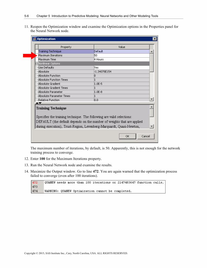
11. Reopen the Optimization window and examine the Optimization options in the Properties panel for the Neural Network node.

The maximum number of iterations, by default, is 50. Apparently, this is not enough for the network training process to converge.

12. Enter 100 for the Maximum Iterations property.

13. Run the Neural Network node and examine the results.

14. Maximize the Output window. Go to line 472. You are again warned that the optimization process failed to converge (even after 100 iterations).




Curiously, increasing the maximum number of iterations changes none of the fit statistics. How can this be? The answer is found in the Iteration Plot window.

16. Examine the Iteration Plot window.

The iteration plot shows the average squared error versus optimization iteration. A massive divergence in training and validation average squared error occurs near iteration 14, indicated by the vertical blue line.



The rapid divergence of the training and validation fit statistics is cause for concern. This primarily results from a large number of weights in the fitted neural network model. The huge number of weights comes from the use of all inputs in the model. Reducing the number of modeling inputs reduces the number of modeling weights and possibly improves model performance.

17. Close the Results window.

5.2 Input Selection

The Neural Network tool in SAS Enterprise Miner lacks a built-in method for selecting useful inputs. Although sequential selection procedures such as stepwise are known for neural networks, the computational costs of their implementation tax even fast computers. Therefore, these procedures are not part of SAS Enterprise Miner. You can solve this problem by using an external process to select useful inputs. In this demonstration, you use the variables selected by the standard regression model. (In Chapter 9, several other approaches are shown.)

19

Copyr i g ht © 2014, SAS Ins t i tu t e Inc . A l l r ights reser ve d .

Model Essentials – Neural NetworksPrediction

formula

Best modelfrom sequence

Sequentialselection

Predict new cases.

Select useful inputs

Optimize complexity.

Select useful inputs. None

5.2 Input Selection 5-9


20

Copyr i g ht © 2014, SAS Ins t i tu t e Inc . A l l r ights reser ve d .

5.01 Multiple Answer PollWhich of the following are true about neural networks in SAS Enterprise Miner?

a. Neural networks are universal approximators.b. Neural networks have no internal, automated process

for selecting useful inputs.c. Neural networks are easy to interpret and thus are

very useful in highly regulated industries.d. Neural networks cannot model nonlinear relationships.



5.3 Selecting Neural Network Inputs This demonstration shows how to use a logistic regression to select inputs for a neural network.

" Additional dimension reduction techniques are discussed in Chapter 9.

1. Delete the connection between the Impute node and the Neural Network node.

2. Connect the Regression node to the Neural Network node.

3. Right-click the Neural Network node and select Update from the pop-up menu.

5.3 Selecting Neural Network Inputs 5-11


4. Open the Variables dialog box for the Neural Network node. Select the check box next to Label and resize the fields for better visibility.

Only the inputs selected by the Regression node's stepwise procedure are not rejected.

5. Close the Variables dialog box.




The Fit Statistics window shows an improvement in model fit using only 19 weights.

The validation and training average squared errors are nearly identical.

5.4 Increasing Network Flexibility 5-13


5.4 Increasing Network Flexibility Stopped training helps ensure that a neural network does not overfit (even when the number of network weights is large). Further improvement in neural network performance

can be realized by increasing the number of hidden units from the default of three. The following are two ways to explore alternative network sizes: • manually, by changing the number of weights by hand • automatically, by using the AutoNeural tool

Changing the number of hidden units manually involves trial-and-error guessing of the “best” number of hidden units. Several hidden unit counts were tried in advance. One of the better selections is demonstrated.

1. Select Network ! in the Neural Network Properties panel.



The Network window appears.

2. Enter 6 as the Number of Hidden Units value.

3. Click OK.


5.4 Increasing Network Flexibility 5-15


The Fit Statistics window shows good model performance on both the average squared error and misclassification scales.

The iteration plot shows optimal validation average squared error occurring on iteration 5.

Unfortunately, there is little else of interest to describe this model. (In Chapter 9, a method is shown to give some insight into describing the cases with high primary outcome probability.)



5.5 Using the AutoNeural Tool (Self-Study) The AutoNeural tool offers an automatic way to explore alternative network architectures and hidden unit counts. This demonstration shows how to explore neural networks with increasing hidden unit counts.

1. Click the Model tab.

2. Drag the AutoNeural tool into the diagram workspace.

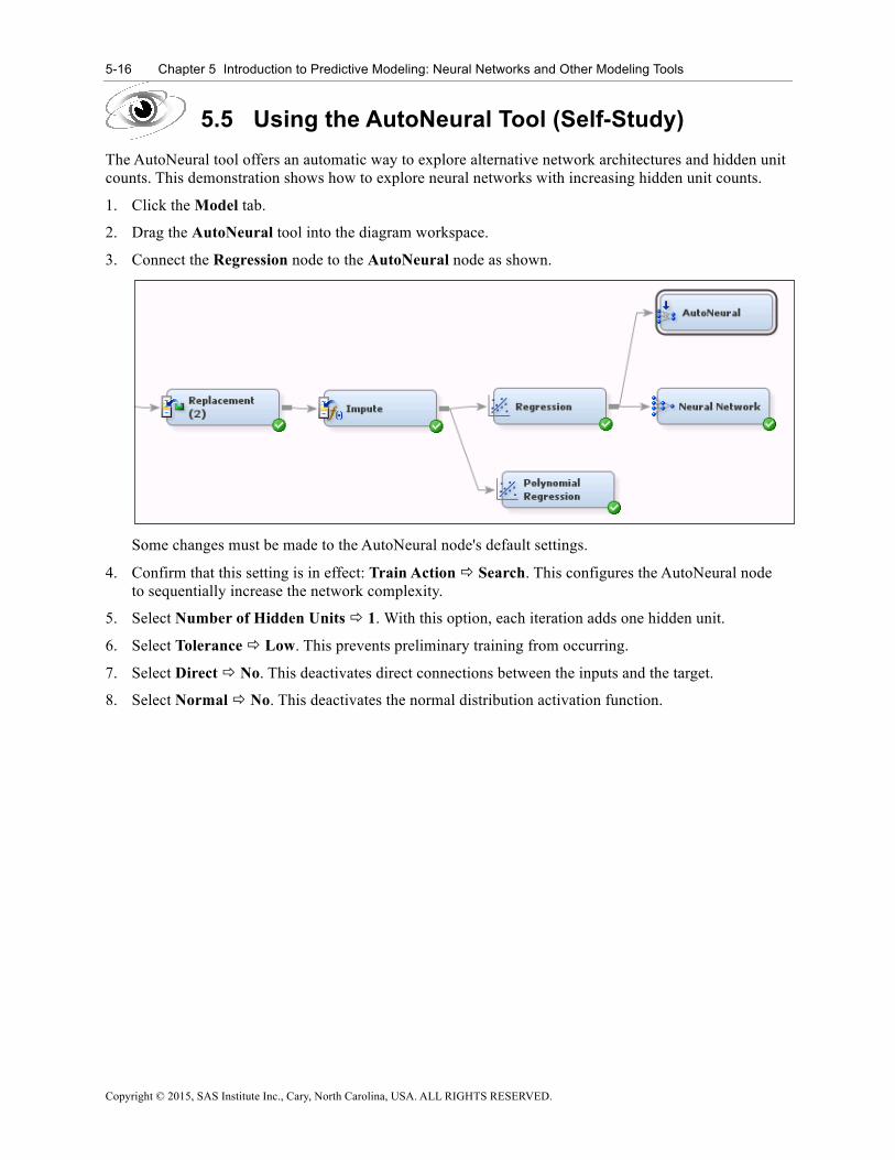
3. Connect the Regression node to the AutoNeural node as shown.

Some changes must be made to the AutoNeural node's default settings.

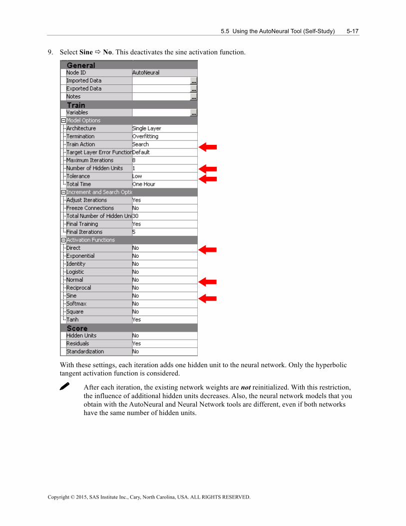
4. Confirm that this setting is in effect: Train Action ! Search. This configures the AutoNeural node to sequentially increase the network complexity.

5. Select Number of Hidden Units ! 1. With this option, each iteration adds one hidden unit.

6. Select Tolerance ! Low. This prevents preliminary training from occurring.

7. Select Direct ! No. This deactivates direct connections between the inputs and the target.

8. Select Normal ! No. This deactivates the normal distribution activation function.

5.5 Using the AutoNeural Tool (Self-Study) 5-17


9. Select Sine ! No. This deactivates the sine activation function.

With these settings, each iteration adds one hidden unit to the neural network. Only the hyperbolic tangent activation function is considered.

" After each iteration, the existing network weights are not reinitialized. With this restriction, the influence of additional hidden units decreases. Also, the neural network models that you obtain with the AutoNeural and Neural Network tools are different, even if both networks have the same number of hidden units.



10. Run the AutoNeural node and view the results. The Results - Node: AutoNeural Diagram window appears.


The number of weights implies that the selected model has one hidden unit. The average squared error and misclassification rates are quite low.



12. Maximize the Iteration Plot window.

The AutoNeural and Neural Network node's iteration plots differ. The AutoNeural node's iteration plot shows the final fit statistic versus the number of hidden units in the neural network.

13. Maximize the Output window. The Output window describes the AutoNeural process.

14. Go to line 52.

These lines show various fit statistics versus training iteration using a single hidden unit network. Training stops at iteration 8 (based on an AutoNeural property setting). Validation misclassification is used to select the best iteration, in this case, Step 3. Weights from this iteration are selected for use in the next step.



15. View output lines 79 - 101.

A second hidden unit is added to the neural network model. All weights related to this new hidden unit are set to zero. All remaining weights are set to the values obtained in iteration 3 above. In this way, the two-hidden-unit neural network (Step 0) and the one-hidden-unit neural network (Step 3) have equal fit statistics.

Training of the two-hidden-unit network begins. The training process trains for eight iterations. Iteration 0 has the smallest validation misclassification and is selected to provide the weight values for the next AutoNeural step.



16. Go to line 106.

The final model training begins. Again iteration zero offers the best validation misclassification.

The next block of output summarizes the training process. Fit statistics from the iteration with the smallest validation misclassification are shown for each step.

The Final Model shows the hidden units added at each step and the corresponding value of the objective function (related to the likelihood).

Chapter 5 Introduction to Predictive Modeling: Neural ... - Neural... · Chapter 5 Introduction to...

Documents

Transcript of Chapter 5 Introduction to Predictive Modeling: Neural ... - Neural... · Chapter 5 Introduction to...