CHAPTER 5. Finite Control Volume Analysis

Applications of Reynolds Transport Theorem a) Conservation of Fluid Mass (Continuity Equation) b) Newton’s 2nd law of fluid motion (Fluid dynamics) c) 1st and 2nd laws of Thermodynamics Note: An assumption through entire chapter,

Flow properties Uniform over cross-sectional areas (CS)

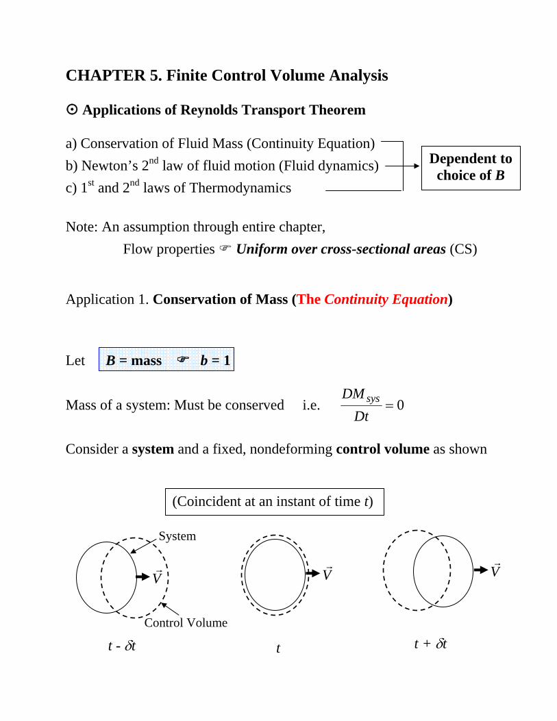
Application 1. Conservation of Mass (The Continuity Equation)

Let B = mass b = 1

Mass of a system: Must be conserved i.e. 0=Dt

DM sys

Consider a system and a fixed, nondeforming control volume as shown

System

Control Volume

Vr

Vr

Vr

t - δt t + δt t

Dependent tochoice of B

(Coincident at an instant of time t)

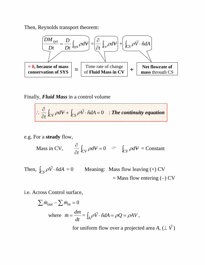
Then, Reynolds transport theorem:

∫= syssys Vd

DtD

DtDM

ρ = ∫∂∂

cv Vdt

ρ + ∫ ⋅CS dAnV ˆr

ρ

Finally, Fluid Mass in a control volume

∴ 0ˆ =⋅+∂∂

∫∫ CSCV dAnVVdt

rρρ : The continuity equation

e.g. For a steady flow,

Mass in CV, 0=∂∂∫CV Vd

tρ ∫CV Vdρ = Constant

Then, ∫ ⋅CS dAnV ˆr

ρ = 0 Meaning: Mass flow leaving (+) CV = Mass flow entering (−) CV

i.e. Across Control surface,

0=−∑∑ inout mm &&

where dtdmm =& = ∫ ⋅A dAnV ˆ

rρ AVQ ρρ == ,

for uniform flow over a projected area A, (⊥ Vr

)

= 0, because of mass conservation of SYS

Time rate of change of Fluid Mass in CV

Net flowrate of mass through CS

= +

Useful analysis tips for Mass Conservation 1. nV ˆ⋅r

over the CS: Negative (−) for flow entering the CV Positive (+) for flow leaving the CV

2. For a steady flow, ∫∂∂

CVVd

tρ = 0

and thus, 0=−=−∑∑ ininoutoutinout QQmm ρρ&&

3. For a steady flow of incompressible fluid (ρ = constant) 0=−=− ∑∑∑∑ ininoutoutinout VAVAQQ

4. For a non-uniform velocity distribution over the CS,

m& = ρAV (V : average value)

5. For more than one steady non-uniform stream,

∑∑∑∑ === ininininoutoutoutout mVAVAm && ρρ

Ex. 1 Fixed and Non-deforming Control Volume

Air flows steadily between two sections in a long, straight portion of 4-in. inside diameter pipe as indicated in figure. The uniformly distributed temperature and pressure at each section are given.

If the average air velocity (nonuniform velocity distribution) at section (2) is 1000 ft/s, calculate the average air velocity at section (1). Sol.) Necessary Eq.: The continuity equation,

∫∂∂

CVVd

tρ + ∫ ⋅

CSdAnV ˆ

rρ = 0 (Steady flow 0=

∂∂∫CV Vd

tρ )

Then, 0ˆ )1(at )2(at =−=⋅∫ inoutCS mmdAnV &&r

ρ

Nonuniform velocity distribution at (1) and (2)

Express the Equation using the Average velocity

VVVAVAmm inout 122111222)1(at )2(at ρρρρ −=−=− &&

or 21

21 VV

ρρ

= (Compressible Air ≠ρ Constant)

Since we know the pressure and temperature at Sections (1) and (2)

∴ 221

122

1

21 V

TpTpVV ==

ρρ (Using the ideal gas law, RTp ρ= )

Ex. 2 Moving and Non-deforming Control Volume An airplane moves forward at a speed of 971 km/h as shown. The

frontal intake area of the jet engine is 0.80 m2 and the entering air density is 0.736 kg/m3. A stationary observer determines that relative to the earth, the jet engine exhaust gases move away from the engine with a speed of 1050 km/h. The engine exhaust area is 0.558 m2, and the exhaust gas density is 0.515 kg/m3. Estimate the mass flowrate of fuel into the engine in kg/h.

In case of moving CV,

DtDM sys = ∫∂

∂CV

Vdt

ρ + ∫ ⋅CS

dAnW ˆr

ρ

where cvVVWrrr

−= : Relative velocity Then, the continuity equation for a moving, nondeforming CV

∴ ∫∂∂

CVVd

tρ + ∫ ⋅

CSdAnW ˆ

rρ = 0

Sol) Necessary Equation: ∫∂∂

CVVd

tρ + ∫ ⋅CS dAnW ˆ

rρ = 0

(Since the air flow relative to moving CV (Engine) is steady, if the air surrounding the engine: Assumed to be stationary.)

Then, ∫ ⋅CS dAnW ˆr

ρ = 0 or 0=−∑∑ inout mm && a) Outflow of mass of CV: 222)2( ˆ AWdAnW ρρ =⋅∫

r

b) Inflow of mass of CV: ∫ ⋅)1( ˆdAnWr

ρ + (Fuel supply)

fuelmAW &+= 111ρ Thus, 222 AWρ 0111 =−− fuelmAW &ρ

∴ fuelm& 222 AWρ= 111 AWρ−

Note: 1W = (Velocity of the air = 0) – (Velocity of plane = − 971 km/h)

= 971 km/h (From left to right) 2W = (Velocity of the exhaust air = 1050 km/h)

– (Velocity of plane = – 971 km/h) = 2021 km/h (From left to right)

C.f. “Deforming” and moving Control Volume : Change in volume size & Control surface movement

∫∂∂

CVVd

tρ + ∫ ⋅

CSdAnW ˆ

rρ = 0: Still applicable

a) 0≠∂∂∫CV Vd

tρ : Boundary of integration changes

b) ∫ ⋅

CSdAnW ˆ

rρ : Determined with W

r

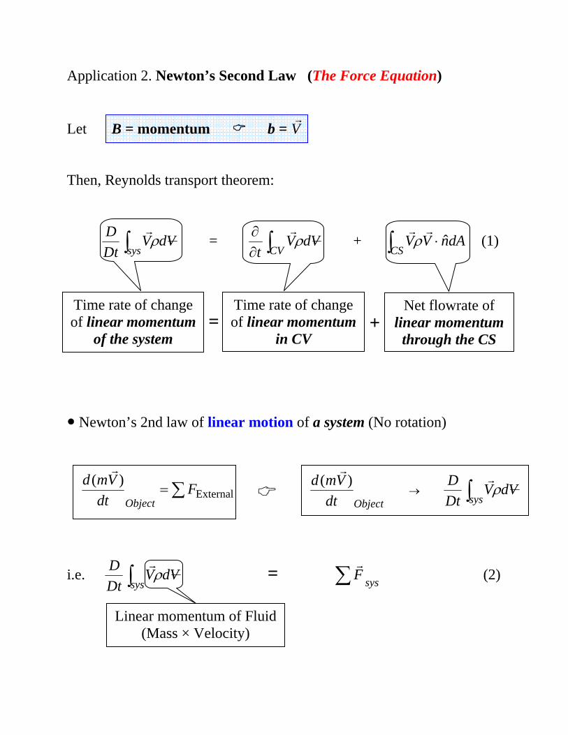
Application 2. Newton’s Second Law (The Force Equation) Let B = momentum b = V

r

Then, Reynolds transport theorem:

∫sysVdV

DtD ρ

r = ∫∂

∂CV

VdVt

ρr

+ ∫ ⋅CS

dAnVV ˆrr

ρ (1)

Newton’s 2nd law of linear motion of a system (No rotation)

i.e. ∫sysVdV

DtD ρ

r = sysF∑

r (2)

Time rate of change of linear momentum

of the system

Time rate of change of linear momentum

in CV

Net flowrate of linear momentum

through the CS

= +

∑= External)( F

dtVmd

Object

r

Linear momentum of Fluid (Mass × Velocity)

ObjectdtVmd )(r

→ ∫sysVdV

DtD ρ

r

Consider a system and a fixed, nondeforming control volume

At the instant of coincidence (Initial instant), ∑ sysF

r= CVcoincidentof Contents∑F

r

By combining Eqs. (1) and (2),

∫∂∂

CVVdV

tρr

+ ∫ ⋅CS

dAnVV ˆrr

ρ = CV coincidentofContents∑Fr

: Linear momentum equation (CV must be in inertial system)

Control Volume analysis for Linear Momentum Conservation Step 1. Choose the appropriate CV.

Step 2. Draw a free-body diagram.

i.e. Find all forces acting on the chosen CV

Step 3. Apply the force equation for each x, y, z components.

∫∑∂∂

= CVx Vdut

F ρ + ∫ ⋅CS dAnVu ˆr

ρ : x-component

∫∑∂∂

= CVy Vdvt

F ρ + ∫ ⋅CS dAnVv ˆr

ρ : x-component

∫∑∂∂

= CVx Vdwt

F ρ + ∫ ⋅CS dAnVw ˆr

ρ : x-component

where kwjviuV ˆˆˆ ++=r

Step 4. Check the steadiness of flow.

i.e. In case of a steady flow, 0=∂∂∫CV VdV

tρr

Step 5. Use the boundary conditions to determine the velocity on CS

(inlets and outlets, etc.)

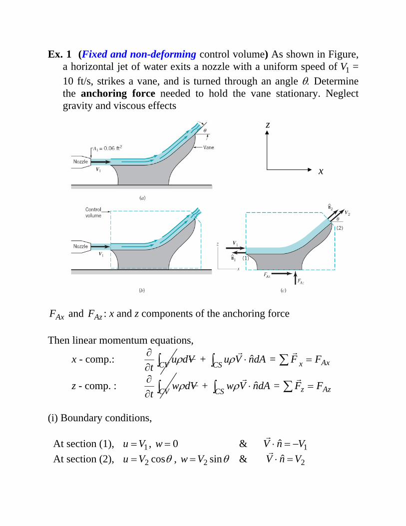
Ex. 1 (Fixed and non-deforming control volume) As shown in Figure, a horizontal jet of water exits a nozzle with a uniform speed of 1V = 10 ft/s, strikes a vane, and is turned through an angle θ. Determine the anchoring force needed to hold the vane stationary. Neglect gravity and viscous effects

AxF and AzF : x and z components of the anchoring force Then linear momentum equations,

x - comp.: ∫∂∂

CV Vdut

ρ + ∫ ⋅CS dAnVu ˆr

ρ = Axx FF =∑r

z - comp. : ∫∂∂

CV Vdwt

ρ + ∫ ⋅CS dAnVw ˆr

ρ = Azz FF =∑r

(i) Boundary conditions, At section (1), 1Vu = , 0=w & 1ˆ VnV −=⋅

r

At section (2), θcos2Vu = , θsin2Vw = & 2ˆ VnV =⋅r

x

z

(ii) In addition, Bernoulli eq. between sections (1) & (2)

22

2212

11 21

21 zVpzVp γργρ ++=++

where 021 == pp : Atmospheric pressure 21 zz γγ = : Neglect the gravity effect (Special case) Then, 21 VV = Inserting all values to the linear momentum equations,

211111)2()1( cos)(ˆˆ AVVAVVdAnVudAnVu θρρρρ +−=⋅+⋅ ∫∫rr

AxF=

21111)2()1( sin)()0(ˆˆ AVVAVdAnVudAnVu θρρρρ +−=⋅+⋅ ∫∫

rr AzF=

(iii) From the continuity equation, 2211 VAVA = → 21 AA = , since 21 VV = Finally, ∴ AxF = 1

211

211

21 )1(coscos AVAVAV ρθθρρ −=+−

AzF = 1

21sin AVθρ

Note. a) If 0=θ (Flat vane), 0== AzAx FF (No anchoring force) b) If o90=θ (Jet: ), AzAx FF −= : Negative c) If o180=θ (Vertical vane), AxF : Negative & AzF = 0

Ex. 2. (Inertially moving, nondeforming control volume) A vane on wheels moves with constant velocity 0V

rwhen a stream of water

having a nozzle exit velocity of 1Vr

is turned by the vane as indicated in figure. Determine the magnitude and direction of the force, F

r,

exerted by the stream of water on the vane surface. The speed of the water jet leaving the nozzle is 100 ft/s, and the vane is moving to the right with a constant speed of 20 ft/s.

Case of an “inertial”, “moving”, nondeforming control volume - Coincident at an initial time

Reynolds transport theorem (Chap. 4),

∫sysVdV

DtD ρ

r = ∫∂

∂CV

VdVt

ρr

+ ∫ ⋅CS

dAnWV ˆrr

ρ

where cvVVW

rrr−= : Relative velocity

Then, linear momentum equation;

CVcoincident of Contents∑Fr

= ∫∂∂

CVVdV

tρr

+ ∫ ⋅CS

dAnWV ˆrr

ρ

= ( )∫ +∂∂

CV CV VdVWt

ρrr

+ ( )∫ ⋅+CS CV dAnWVW ˆ

rrrρ

(since Inertial CV Constant CVVr

Steady flow) In addition, ( )∫ ⋅+

CS CV dAnWVW ˆrrr

ρ = ∫ ⋅CS

dAnWW ˆrr

ρ + ∫ ⋅CSCV dAnWV ˆ

rrρ

Finally, for an inertial, moving, nondeforming control volume

∴ ∫ ⋅CS

dAnWW ˆrr

ρ = CVcoincidentofContents∑Fr

since the continuity equation for a steady flow,

∫∂∂

CVVd

tρ + ∫ ⋅

CSdAnW ˆ

rρ = 0

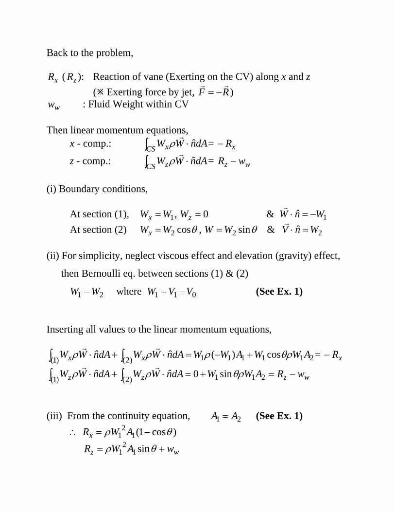
Back to the problem,

xR ( zR ): Reaction of vane (Exerting on the CV) along x and z ( Exerting force by jet, RF

rr−= )

ww : Fluid Weight within CV Then linear momentum equations,

x - comp.: ∫ ⋅CS x dAnWW ˆr

ρ = xR−

z - comp.: ∫ ⋅CS z dAnWW ˆr

ρ = wz wR − (i) Boundary conditions, At section (1), 1WWx = , 0=zW & 1ˆ WnW −=⋅

r

At section (2) θcos2WWx = , θsin2WW = & 2ˆ WnV =⋅r

(ii) For simplicity, neglect viscous effect and elevation (gravity) effect,

then Bernoulli eq. between sections (1) & (2)

21 WW = where 011 VVW −= (See Ex. 1) Inserting all values to the linear momentum equations,

211111)2()1( cos)(ˆˆ AWWAWWdAnWWdAnWW xx θρρρρ +−=⋅+⋅ ∫∫rr

= xR−

wzzz wRAWWdAnWWdAnWW −=+=⋅+⋅ ∫∫ 211)2()1( sin0ˆˆ θρρρrr

(iii) From the continuity equation, 21 AA = (See Ex. 1) ∴ =xR )cos1(1

21 θρ −AW

=zR wwAW +θρ sin12

1