Chapter 5: Engineering Cost Estimates Synopsis · 5-1 Chapter 5: Engineering Cost Estimates...
34
5-1 Chapter 5: Engineering Cost Estimates Synopsis This chapter summarizes the data sources and methodology used to estimate the engineering costs of attaining the alternative more stringent levels for the ozone primary standard analyzed in this RIA. This chapter estimates the engineering costs of 0.065 ppm, 0.070 ppm, 0.075 ppm, and 0.079 ppm. The chapter presents engineering cost estimates for the illustrative modeled control strategy outlined in Chapter 3 (which uses currently available known controls). The modeled control strategy discussion is followed by a presentation of estimates for the engineering costs of the additional tons of emissions that are needed to move to full attainment of the alternate standards analyzed, referred to as Extrapolated Costs (methodology and numbers discussed in Chapter 4). As noted in Chapter 3, EPA first modeled an illustrative control strategy aimed at attaining a tighter standard of 0.070 ppm in 2020. EPA modeled the lower end of the proposed range to capture a larger number of geographic areas that may be affected by a new ozone standard. These known controls were insufficient to bring all areas into attainment with 0.070 ppm, and EPA then developed methodology to estimate additional tons of emissions needed to attain 0.079 ppm, 0.075 ppm, 0.070 ppm, and 0.065 ppm. This chapter presents the engineering costs associated with each portion of the control analysis, clearly identifying the relative engineering costs of modeled versus extrapolated emissions reductions as well as providing an estimate of the total engineering cost of attainment nationwide in 2020. Nationwide attainment refers to all areas of the nation that are required to attain the current ozone standard by the year 2020. It does not reflect full attainment for the two areas of California, which have attainment dates for the current standard post 2020. For a complete discussion attainment for these two areas of California see Appendix 7b. Section 5.1 summarizes the methodology and the engineering costs associated with applying known and supplemental controls to partially attain a 0.070 ppm alternative standard, incremental to reaching the current baseline (effectively 0.084 ppm) in 2020. Section 5.2 describes the methodology used to estimate the engineering costs of extrapolated tons needed to reach attainment of the final 0.075 ppm standard as well as the three alternatives and provides estimates of how much additional engineering costs will be associated with moving from the modeled partial attainment scenario (i.e. modeled control strategy) to the nationwide attainment scenario (see Chapter 4 for discussion of extrapolated tons needed to attain 0.079, 0.075, 0.070, and 0.065 ppm). The engineering costs described in this chapter generally include the costs of purchasing, installing, and operating the referenced technologies. For a variety of reasons, actual control costs may vary from the estimates EPA presents here. As discussed throughout this report, the technologies and control strategies selected for analysis are illustrative of one way in which nonattainment areas could meet a revised standard. There are numerous ways to construct and evaluate potential control programs that would bring areas into attainment with alternative standards, and EPA anticipates that state and local governments will consider programs that are best suited for local conditions. Furthermore, based on past experience, EPA believes that it is reasonable to anticipate that the marginal cost of control will decline over time due to
Transcript of Chapter 5: Engineering Cost Estimates Synopsis · 5-1 Chapter 5: Engineering Cost Estimates...

5-1
Chapter 5: Engineering Cost Estimates
Synopsis
This chapter summarizes the data sources and methodology used to estimate the engineering costs of attaining the alternative more stringent levels for the ozone primary standard analyzed in this RIA. This chapter estimates the engineering costs of 0.065 ppm, 0.070 ppm, 0.075 ppm, and 0.079 ppm. The chapter presents engineering cost estimates for the illustrative modeled control strategy outlined in Chapter 3 (which uses currently available known controls). The modeled control strategy discussion is followed by a presentation of estimates for the engineering costs of the additional tons of emissions that are needed to move to full attainment of the alternate standards analyzed, referred to as Extrapolated Costs (methodology and numbers discussed in Chapter 4).
As noted in Chapter 3, EPA first modeled an illustrative control strategy aimed at attaining a tighter standard of 0.070 ppm in 2020. EPA modeled the lower end of the proposed range to capture a larger number of geographic areas that may be affected by a new ozone standard. These known controls were insufficient to bring all areas into attainment with 0.070 ppm, and EPA then developed methodology to estimate additional tons of emissions needed to attain 0.079 ppm, 0.075 ppm, 0.070 ppm, and 0.065 ppm. This chapter presents the engineering costs associated with each portion of the control analysis, clearly identifying the relative engineering costs of modeled versus extrapolated emissions reductions as well as providing an estimate of the total engineering cost of attainment nationwide in 2020. Nationwide attainment refers to all areas of the nation that are required to attain the current ozone standard by the year 2020. It does not reflect full attainment for the two areas of California, which have attainment dates for the current standard post 2020. For a complete discussion attainment for these two areas of California see Appendix 7b. Section 5.1 summarizes the methodology and the engineering costs associated with applying known and supplemental controls to partially attain a 0.070 ppm alternative standard, incremental to reaching the current baseline (effectively 0.084 ppm) in 2020.
Section 5.2 describes the methodology used to estimate the engineering costs of extrapolated tons needed to reach attainment of the final 0.075 ppm standard as well as the three alternatives and provides estimates of how much additional engineering costs will be associated with moving from the modeled partial attainment scenario (i.e. modeled control strategy) to the nationwide attainment scenario (see Chapter 4 for discussion of extrapolated tons needed to attain 0.079, 0.075, 0.070, and 0.065 ppm).
The engineering costs described in this chapter generally include the costs of purchasing, installing, and operating the referenced technologies. For a variety of reasons, actual control costs may vary from the estimates EPA presents here. As discussed throughout this report, the technologies and control strategies selected for analysis are illustrative of one way in which nonattainment areas could meet a revised standard. There are numerous ways to construct and evaluate potential control programs that would bring areas into attainment with alternative standards, and EPA anticipates that state and local governments will consider programs that are best suited for local conditions. Furthermore, based on past experience, EPA believes that it is reasonable to anticipate that the marginal cost of control will decline over time due to

5-2
technological improvements and more widespread adoption of previously niche control technologies. Also, EPA recognizes the extrapolated portion of the engineering cost estimates reflects substantial uncertainty about which sectors, and which technologies, might become available for cost-effective application in the future. This is explained in further detail in Section 5.3. Appendix 5a includes detailed cost and control efficiency information on different control measures applied as part of our modeled control strategy, and also includes summary results from applications of specific control measures.
It is also important to recognize that the engineering cost estimates are limited in their scope. Because we is not certain of the specific actions that states will take to design State Implementation Plans to meet the revised standards, we do not present estimated costs that government agencies may incur for managing the requirement and implementation of these control strategies or for offering incentives that may be necessary to encourage or motivate the implementation of the technologies, especially for technologies that are not necessarily market driven. This analysis does not assume specific control measures that would be required in order to implement these technologies on a regional or local level.
We use EMPAX-CGE to estimate the economic impacts and the social costs associated with the modeled control strategy. EMPAX uses as input the engineering costs estimated for the modeled control strategy to calculate its economic impacts and social costs. Economic impacts are estimates of changes in price and output for those industries and consumers of their output affected by the modeled control strategy. Social costs are costs from changes in household welfare due to impacts from the costs of the controls in the modeled control strategy. For more details on the economic impacts and social costs, please refer to Appendix 5b.
5.1 Modeled Controls
5.1.1 Sector Methodology
5.1.1.1 NonEGU Point and Area Sources: AirControlNET
After designing a national hypothetical control strategy using the methodology discussed in Chapter 3 (see sub-section 3.2.1), EPA used AirControlNET to estimate engineering control costs. AirControlNET calculates engineering costs using three different methods: (1) by multiplying an average annualized cost per ton estimate against the total tons of a pollutant reduced to derive a total cost estimate; (2) by calculating cost using an equation that incorporates information regarding key plant information; or (3) by using both cost per ton and cost equations. Most control cost information within AirControlNET has been developed based on the cost per ton approach. This is because estimating engineering costs using an equation requires more data, and parameters used in other non-cost per ton methods may not be readily available or broadly representative across sources within the emissions inventory. The costing equations used in AirControlNET require either plant capacity or stack flow to determine annual, capital and/or operating and maintenance (O&M) costs. Capital costs are converted to annual costs, in dollars

5-3
per ton, using the capital recovery factor.1 Where possible cost calculations are used to calculate total annual control cost (TACC) which is a function of the capital (CC) and O&M costs. Capital costs are converted to annual costs, in dollars per ton, using the capital recovery factor (CRF). The capital recovery factor incorporates the interest rate and equipment life (in years) of the control equipment. Operating costs are calculated as a function of annual O&M and other variable costs. The resulting TACC equation is TACC = (CRF * CC) + O&M.
Engineering costs will differ based upon quantity of emissions reduced, plant capacity, or stack flow which can vary by emissions inventory year. Engineering costs will also differ by the year the costs are calculated for (i.e., 1999$ versus 2006$). For capital investment, we do not assume early capital investment in order to attain standards by 2020. For 2020, our estimate of annualized costs represents a “snapshot” of the annualized costs, which include annualized capital and O&M costs, for those controls included in our modeled control strategy. Our engineering cost analysis uses the equivalent uniform annual costs (EUAC) method, in which annualized costs are calculated based on the equipment life for the control measure along with the interest rate by use of the CRF as mentioned previously in this chapter. Annualized costs are estimated as equal for each year the control is expected to operate. Hence, our annualized costs for nonEGU point and area sources estimated for 2020 are the same whether the control measure is installed in 2019 or in 2010. We make no presumption of additional capital investment in years beyond 2020. The EUAC method is discussed in detail in the EPA Air Pollution Control Cost Manual (found at http://epa.gov/ttn/catc/products.html#cccinfo). Applied controls and their respective engineering costs are provided in the Ozone NAAQS RIA docket.
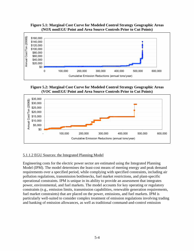
The modeled control strategy for nonEGU Point and Area sources incorporated annualized engineering cost per ton caps. These caps were defined as the upper cost per ton for controls of nonEGU point and area sources. The caps were calculated by examining the marginal cost curves for each pollutant for the geographic areas (approximately 1,300 counties for NOx controls, see Figure 3.5 and approximately 120 counties for VOC controls, see Figure 3.6) being analyzed for this analysis. For reductions of NOx emissions the cap (see Figure 5.1) was set at $23,000/ton (2006$). At this cap, ninety-eight percent of the possible reductions from known measures are achieved at eighty-two percent of the total annualized engineering cost. There were only two controls whose cost per ton were greater than this cap, and subsequently not included in this analysis, due to the large capital component of installing these controls. A similar process was followed for reductions from VOCs. The relative air quality effectiveness of reductions in VOC was considered, and the marginal cost curve (Figure 5.2) was analyzed. Subsequently, the cap was set at approximately $5,000/ton (2006$). At this cap, forty-six percent of the possible reductions are achieved at fifteen percent of the total engineering cost. It is important to note that as part of the extrapolated cost analysis the VOC cap was raised to $15,000/ton (for geographic areas where the supplemental air quality modeling showed VOC control to be beneficial). At this cap (2006$) ninety-eight percent of the possible reductions could be achieved.
1 For more information on this cost methodology and the role of AirControlNET, see Section 6 of the 2006 PM RIA, AirControlNET 4.1 Control Measures Documentation (Pechan, 2006b), or the EPA Air Pollution Control Cost Manual, Section 1, Chapter 2, found at http://www.epa.gov/ttn/catc/products.html#cccinfo.
5-4
Figure 5.1: Marginal Cost Curve for Modeled Control Strategy Geographic Areas (NOX nonEGU Point and Area Source Controls Prior to Cut Points)
$0$20,000$40,000$60,000$80,000
$100,000$120,000$140,000$160,000
0 100,000 200,000 300,000 400,000 500,000 600,000
Cumulative Emission Reductions (annual tons/year)
Ann
ual C
ost/T
on (2
006$
)
Figure 5.2: Marginal Cost Curve for Modeled Control Strategy Geographic Areas (VOC nonEGU Point and Area Source Controls Prior to Cut Points)
$0$5,000
$10,000$15,000$20,000$25,000$30,000$35,000
- 100,000 200,000 300,000 400,000 500,000 600,000
Cumulative Emission Reductions (annual tons/year)
Ann
ual C
ost/T
on (2
006$
)
5.1.1.2 EGU Sources: the Integrated Planning Model
Engineering costs for the electric power sector are estimated using the Integrated Planning Model (IPM). The model determines the least-cost means of meeting energy and peak demand requirements over a specified period, while complying with specified constraints, including air pollution regulations, transmission bottlenecks, fuel market restrictions, and plant-specific operational constraints. IPM is unique in its ability to provide an assessment that integrates power, environmental, and fuel markets. The model accounts for key operating or regulatory constraints (e.g., emission limits, transmission capabilities, renewable generation requirements, fuel market constraints) that are placed on the power, emissions, and fuel markets. IPM is particularly well-suited to consider complex treatment of emission regulations involving trading and banking of emission allowances, as well as traditional command-and-control emission

5-5
policies.2 Applied controls and their respective engineering costs are provided in the docket. IPM is described in further detail in Appendix 3.
5.1.1.3 Onroad and Nonroad Mobile Sources: National Mobile Inventory Model (NMIM) and Various Studies
Engineering cost information for mobile source controls was taken from studies conducted by EPA for previous rulemakings and studies conducted for development of voluntary and local measures that could be used by state or local programs to assist in improving air quality. Applied controls and their respective engineering costs are provided in the docket.3
Engineering costs, in terms of dollars per ton emissions reduced, were applied to emission reductions calculated for the onroad and nonroad mobile sectors that were generated using the NMIM. NMIM is an EPA model for estimating pollution from highway vehicles and nonroad mobile equipment. NMIM uses current versions of EPA’s model for onroad mobile sources, MOBILE6, and nonroad mobile sources, NONROAD, to calculate emission inventories 4.
5.1.2 Modeled Controls—Engineering Cost by Sector
In this section, we provide engineering cost estimates of the control strategies identified in Chapter 3 that include control technologies on nonEGU stationary sources, area sources, EGUs, and onroad and nonroad mobile sources. Engineering costs generally refer to the capital equipment expense, the site preparation costs for the application, and annual operating and maintenance costs.
The total annualized cost of control in each sector in the control scenario is provided in Table 5.1. These numbers reflect the engineering costs across sectors annualized at a discount rate of 7% and 3%, consistent with the guidance provided in the Office of Management and Budget’s (OMB) (2003) Circular A-4. However, it is important to note that it is not possible to estimate both 7% and 3% discount rates for each source (see section 5.1.3). In Table 5.1, an annualized control cost is provided to allow for comparison across sectors, and between costs and benefits. A 7% discount rate was used for control measures applied to nonEGU point, area,
2 The application of the 0.070 EGU control strategy results in annual NOx allowance price decreasing from $1618/ton in the baseline to $641/ton. See Technical Support Document on EGU Control Strategies for more details. Further detailed information on IPM is available in Section 6 of the 2006 PM RIA or at http://www.epa.gov/airmarkets/epa-ipm 3 The expected emissions reductions from SCR retrofits are based on data derived from EPA regulations (Control of Emissions of Air Pollution from 2004 and Later Model Year Heavy-duty Highway Engines and Vehicles published October 2000), interviews with component manufacturers, and EPA’s Summary of Potential Retrofit Technologies available at www.epa.gov/otaq/retrofit/retropotentialtech.htm. For more information on mobile idle reduction technologies (MIRTs) see EPA’s Idle Reduction Technology page at http://www.epa.gov/otaq/smartway/idlingtechnologies.htm. 4 More information regarding the National Mobile Inventory Model (NMIM) can be found at
http://www.epa.gov/otaq/nmim.htm

5-6
and mobile sources. Engineering costs from EGU sources, which are calculated using the IPM model and variable interest rates, are captured in this table at an annualized 7% discount rate.5
5 A different plant-specific interest rate is applied in estimating control costs within IPM. See PM
RIA for details.

5-7
Table 5.1: Annual Control Costs by Sector and Region, for the Modeled Control Strategy (2006$) a, b, e
Modeled Control Strategy
Engineering Cost by Region (M 2006$)
Source Category East West CA
Total Cost (M 2006$)
Average Cost/Ton (2006$)
Electric Generating Units (EGU) Sector Controls for NOx cap and trade program and local measures in projected nonattainment areas for coal units.
$170 $(70) c $66 $160 $1,900 f
Total $170 $(70) $66 $160 Mobile Source Sector
Onroad Sources (Ex: automobiles, buses, trucks, and motorcycles traveling on roads and highways)
$360 $55 $45 $460 $2,100
Nonroad Sources (Ex: railroad locomotives; marine vessels, aircraft, and farm, construction, industrial and lawn/garden equipment)
$150 $21 $16 $190 $3,400
Total $510 $75 $61 $650 NonEGU Sector
Point Sources (Ex: chemical manufacturing, cement manufacturing, petroleum refineries, and iron and steel mills)
$1,400 $57 $4.7 $1,500 $3,800
Area Sector Area Sources (Ex: residential woodstoves, agriculture) $480 $44 $20 $550 $1,900
Total $2,000 Total Annualized Costs (using a 7% interest rate) $2,600 $170 $160 $2,800
Total Annualized Costs (using a 3% interest rate) d
$2,400 $160 $160 $2,600
a All estimates rounded to two significant figures. As such, totals will not sum down columns. The modeled control strategy is that strategy applied to reach attainment of the 0.070 alternate primary standard, and is described in detail in Chapter 3.
b All estimates provided reflect the engineering cost of the modeled control strategy, incremental to a 2020 baseline of compliance with the current standard of 0.084 ppm.
c The total cost is negative in the west for the modeled control strategy due to an electricity generation shift. The west generates less electricity and exports from the east.
d Total annualized costs were calculated using a 3% discount rate for controls which had a capital component and where equipment life values were available. For this modeled control strategy, data for calculating annualized costs at a 3% discount was only available for NonEGU point sources. Therefore, the total annualized cost value presented in this referenced cell is an aggregation of engineering costs at 3% and 7% discount rate.
e These estimates do not reflect benefits or costs for the San Joaquin Valley or South Coast Air Basins. Please see Appendix 7b for analysis of these areas.
5-8
f This average cost/ton estimate is based on ozone season NOx reductions from EGUs from controls that operate year-round as explained in Chapter 3. By counting NOx reductions in the ozone season while operation of NOx controls is modeled as year-round, our cost/ton estimate may spread out reductions and thus affect the average cost/ton estimate. It should be noted that the resulting cost/ton of the controls applied within EGU control strategy is practically the same as that in 2020 for the final CAIR rule ($1,900 in 2006 dollars).
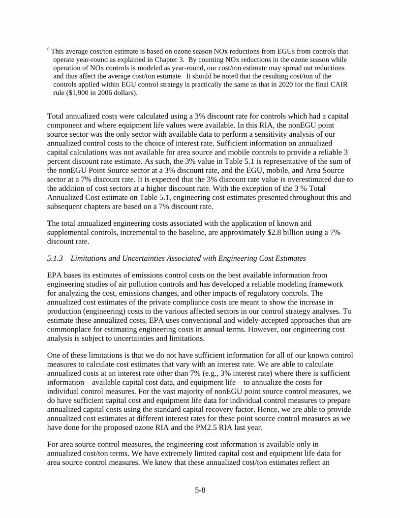
Total annualized costs were calculated using a 3% discount rate for controls which had a capital component and where equipment life values were available. In this RIA, the nonEGU point source sector was the only sector with available data to perform a sensitivity analysis of our annualized control costs to the choice of interest rate. Sufficient information on annualized capital calculations was not available for area source and mobile controls to provide a reliable 3 percent discount rate estimate. As such, the 3% value in Table 5.1 is representative of the sum of the nonEGU Point Source sector at a 3% discount rate, and the EGU, mobile, and Area Source sector at a 7% discount rate. It is expected that the 3% discount rate value is overestimated due to the addition of cost sectors at a higher discount rate. With the exception of the 3 % Total Annualized Cost estimate on Table 5.1, engineering cost estimates presented throughout this and subsequent chapters are based on a 7% discount rate.
The total annualized engineering costs associated with the application of known and supplemental controls, incremental to the baseline, are approximately $2.8 billion using a 7% discount rate.
5.1.3 Limitations and Uncertainties Associated with Engineering Cost Estimates
EPA bases its estimates of emissions control costs on the best available information from engineering studies of air pollution controls and has developed a reliable modeling framework for analyzing the cost, emissions changes, and other impacts of regulatory controls. The annualized cost estimates of the private compliance costs are meant to show the increase in production (engineering) costs to the various affected sectors in our control strategy analyses. To estimate these annualized costs, EPA uses conventional and widely-accepted approaches that are commonplace for estimating engineering costs in annual terms. However, our engineering cost analysis is subject to uncertainties and limitations.
One of these limitations is that we do not have sufficient information for all of our known control measures to calculate cost estimates that vary with an interest rate. We are able to calculate annualized costs at an interest rate other than 7% (e.g., 3% interest rate) where there is sufficient information—available capital cost data, and equipment life—to annualize the costs for individual control measures. For the vast majority of nonEGU point source control measures, we do have sufficient capital cost and equipment life data for individual control measures to prepare annualized capital costs using the standard capital recovery factor. Hence, we are able to provide annualized cost estimates at different interest rates for these point source control measures as we have done for the proposed ozone RIA and the PM2.5 RIA last year.
For area source control measures, the engineering cost information is available only in annualized cost/ton terms. We have extremely limited capital cost and equipment life data for area source control measures. We know that these annualized cost/ton estimates reflect an

5-9
interest rate of 7% because these estimates are typically products of technical memos and reports prepared as part of rules issued by our office (OAQPS) over the last 10 years or so, and the costs estimated in these reports have followed the policy provided in OMB Circular A-4 that recommends the use of 7% as the interest rate for annualizing regulatory costs. Capital cost
Figure 5.3: Total Annualized Costs by Emissions Sector and Region for Modeled Control Strategy in 2020a, b, c, d
-$0.10
$0.10
$0.30
$0.50
$0.70
$0.90
$1.10
$1.30
$1.50
Tota
l Cos
ts (B
200
6$)
East West CA
Area nonEGU Point EGU Onroad Nonroad
a Total costs presented above are for a seven percent discount rate. b All estimates provided reflect the engineering cost of the modeled control strategy, incremental to a
2020 baseline of compliance with the current standard of 0.084 ppm. c The total cost is negative in the west for the modeled control strategy due to an electricity generation
shift. The west generates less electricity and exports from the east. d These estimates do not reflect benefits or costs for the San Joaquin Valley or South Coast Air Basins.
Please see Appendix 7b for analysis of these areas.
information for these area source controls, however, is often limited since these measures are often not the traditional add-on controls where the capital cost is well known and convenient to estimate. Such area source controls can include reformulation of coatings to reduce VOC, as one example. The limited availability of useful capital cost data for such control measures has led to our use of annualized cost/ton estimates to represent the engineering costs of these controls in our cost tools and hence in the PM2.5 and ozone RIAs.

5-10
For mobile source measures, the situation is very much like that for our area source measures. We do not have sufficient capital cost information from what our mobile source office (OTAQ) has sent us to compute annualized costs for different interest rates other than 7%. Finally, It should be noted that the annualized capital costs for EGUs are prepared at an interest rate other than 7%. Information on the annualization of EGU control costs is presented later in this chapter.
There are some unquantified costs that are not adequately captured in this illustrative analysis. These costs include the costs of federal and State administration of control programs, which we believe are less than the alternative of States developing approvable SIPs, securing EPA approval of those SIPs, and Federal/State enforcement. Additionally, control measure costs referred to as “no cost” may require limited government agency resources for administration and oversight of the program not included in this analysis; those costs are generally outweighed by the saving to the industrial, commercial, or private sector. The Agency also did not consider transactional costs and/or effects on labor supply in the illustrative analysis.
The economic impacts of the cost of these modeled control strategy is included in Appendix 5b of this analysis. The illustrative analysis does quantify the potential for advancements in the capabilities of pollution control technologies as well as reductions in their engineering costs over time. This is discussed in Section 5.4.
For purposes of this analysis, we assume attainment by 2020 for all areas except San Joaquin Valley and South Coast air basins in California. The state has submitted plans to EPA for implementing the current ozone standard which propose that these two areas of California meet that standard by 2024. We have assumed for analytical purposes that the San Joaquin Valley and South Coast air basin would attain a new standard in 2030. There are many uncertainties associated with the year 2030 analysis. Between 2020 and 2030 several federal air quality rules are likely to further reduce emissions of NOx and VOC, such as, but not limited to National rules for Diesel Locomotives, Diesel Marine Vessels, and Small Nonroad Gasoline Engines. These emission reductions should lower ambient levels of ozone in California between 2020 and 2030. Complete emissions inventories as well as air quality modeling were not available for this year 2030 analysis. Due to these limitations, it is not possible to adequately model 2030 air quality changes that are required to develop robust controls strategies with associated costs and benefits. In order to provide a rough approximation of the costs and benefits of attaining 0.075 ppm and the alternate standards in San Joaquin and South Coast air basins, we’ve relied on the available data. Available data includes emission inventories, which do not include any changes in stationary source emissions beyond 2020, and 2020 supplemental air quality modeling. This data was used to develop extrapolated costs and benefits of 2030 attainment. To view the complete analysis for the San Joaquin Valley and South Coast air basins see Appendix 7b.3
5.2 Extrapolated Engineering Costs
5.2.1 Methodology
This section presents the methodology and results of the extrapolated engineering cost calculations of attainment of a new ozone standard of 0.075 ppm and analyses of three

5-11
alternative standards, a less stringent 0.079 ppm and two more stringent options (.065 and 0.070 ppm).
As discussed in Chapter 3, the application of the modeled control strategy was not successful in reaching nationwide attainment of the alternate ozone standards. Many areas remained in nonattainment for all four alternate standard scenarios; therefore, the engineering costs detailed in Section 5.1 represent only the costs of partial attainment.
The estimation of engineering costs for unspecified emission reductions needed to reach attainment many years in the future is inherently a difficult issue. As described later in this chapter, our experience with Clean Air Act implementation shows that technological advances and development of innovative strategies can make possible emissions reductions that are unforeseen today, and to reduce costs of emerging technologies over time. But we cannot quantitatively predict the amount of technology advance in the future. For areas needing significant additional emission reductions, much of the control must be for sources that historically haven’t been controlled. The relationship of the cost of such control to the cost of control options available today is not at all clear. Available, current known control measures increase in cost beyond the range of what has ever been implemented and would still not provide the needed additional control for full attainment in the analysis year 2020. In the absence of technological change, the needed control for full attainment in 2020 would not be available.
The degree to which unknown controls are needed to achieve attainment depends significantly upon variables in the analysis, such as attainment date assumptions. We will better understand the true scope of the issue in the future as states conduct detailed area-by-area analyses to determine available controls and attainment dates that are appropriate under the Clean Air Act. We do not attempt to determine specific attainment dates in this analysis. The Clean Air Act provides flexibility for a nonattainment area to receive an attainment date up to 20 years after designation if earlier attainment is not practical based on controls that are reasonably available considering cost. Although we assume attainment in 2020 (except for two California areas), areas that face difficulty attaining could qualify under the Clean Air Act for an attainment date as late as 2030 (assuming designations in 2010). This would give such areas additional time to take advantage for national standards to reduce emissions from onroad and nonroad mobile sources through fleet turnover, and to take advantage of technological innovation in cleaner technologies after 2020.
Prior to presenting the methodology for estimating costs for unspecified emission reductions, it is important to provide information from EPA’s Science Advisory Board Council Advisory,6 dated June 8, 2007, on the issue of estimating costs of unidentified control measures.
812 Council Advisory, Direct Cost Report, Unidentified Measures (charge question 2.a)
“The Project Team has been unable to identify measures that yield sufficient emission reductions to comply with the National Ambient Air Quality Standards (NAAQS) and
6 U.S. Environmental Protection Agency. June 2007. Advisory Council on Clean Air Compliance Analysis (COUNCIL), Council Advisory on OAR’s Direct Cost Report and Uncertainty Analysis Plan. Washington, DC.

5-12
relies on unidentified pollution control measures to make up the difference. Emission reductions attributed to unidentified measures appear to account for a large share of emission reductions required for a few large metropolitan areas but a relatively small share of emission reductions in other locations and nationwide.
“The Council agrees with the Project Team that there is little credibility and hence limited value to assigning costs to these unidentified measures. It suggests taking great care in reporting cost estimates in cases where unidentified measures account for a significant share of emission reductions. At a minimum, the components of the total cost associated with identified and unidentified measures should be clearly distinguished. In some cases, it may be preferable to not quantify the costs of unidentified measures and to simply report the quantity and share of emissions reductions attributed to these measures.
“When assigning costs to unidentified measures, the Council suggests that a simple, transparent method that is sensitive to the degree of uncertainty about these costs is best. Of the three approaches outlined, assuming a fixed cost/ton appears to be the simplest and most straightforward. Uncertainty might be represented using alternative fixed costs per ton of emissions avoided.”
EPA has considered this advice and the requirements of E.O. 12866 and OMB circular A-4, which provides guidance on the estimation of benefits and costs of regulations.
To generate estimates of the costs and benefits of meeting alternative standards, EPA has assumed the application of unspecified future controls that make possible the emissions reductions needed for attainment in 2020 (excluding two California areas). By definition, there is no cost data in existence for unidentified future technologies or innovative strategies.
EPA used two methodologies for estimating the costs of unspecified future controls: a new hybrid methodology and a fixed-cost methodology. Both approaches assume that innovative strategies and new control options make possible the emissions reductions needed for attainment by 2020. The fixed cost methodology was preferred by EPA’s Science Advisory Board over two other options, including a marginal-cost-based approach. The hybrid approach has not yet been reviewed by the SAB.
The hybrid approach creates a marginal cost curve and an average cost curve representing the cost of unknown future controls needed for 2020 attainment. This approach explicitly estimates the average per-ton cost of unspecified emissions reductions assumed for each area, with a higher average cost-per-ton in areas needing a higher proportion of unknown controls relative to known modeled controls. This requires assumptions about the average cost of the least expensive unspecified future controls, and the rate at which the average cost of these controls rises as more extrapolated tons are needed for attainment (relative to the amount of reductions from known, modeled controls). These factors in turn depend on implicit assumptions about future technological progress and innovation in emission reduction strategies.
The fixed cost methodology utilizes a national average cost per ton of future unspecified controls needed for attainment, as well as two sensitivity values (presented in Appendix 5a.4.3). The

5-13
range of estimates reflects different assumptions about the cost of additional emissions reductions beyond those in the modeled control strategy. The alternative estimates implicitly reflect different assumptions about the amount of technological progress and innovation in emission reduction strategies.
The hybrid methodology has the advantage of using the information about how significant the needed reductions from unspecified control technology are relative to the known control measures and matching that with expected increasing per unit cost for going beyond the modeled technology. Under this approach, the relative costs of unspecified controls in different geographic areas reflect the expectation that average per-ton control costs are likely to be higher in areas needing a higher ratio of emission reductions from unspecified and known controls.
The fixed cost methodology reflects a view that because no cost data exists for unspecified future strategies, it is unclear whether approaches using hypothetical cost curves will be more accurate or less accurate in forecasting total national costs of unspecified controls than a fixed-cost approach that uses a range of national cost per ton values.
Technological change will provide new control possibilities that can be employed to provide the additional unspecified control needed to reach attainment. These new technologies will make control possible where control has not been available for estimating our known control. An example might be the development of a new control technology for a type of emissions that have never been controlled. Technological change is also expected to reduce the cost of known controls that currently have prohibitive costs. For example, suppose a source that was not chosen for control because the estimated cost was $60,000 per ton but technological change reduces the cost to $16,000 per ton. Finally, control technologies may change so that higher control efficiencies may be obtained without a significant increase in per unit costs of control.
Both approaches (the hybrid and the fixed) estimate costs using national level parameters and local area information about needed emission reductions. Because cost changes due to technological change will be available on a national level, it makes sense to use national level estimates of these parameters. Local areas have different levels of needed emission reductions and different inventories of uncontrolled emissions and estimates of needed emission reductions are used in both models. The hybrid model also uses information about the amount of modeled control estimated for the local area.
The hybrid approach has yet to be peer reviewed and reflects a range of views about the likely cost of future techniques and strategies that reduce air pollutant emissions. Section 5.4 discusses historical experience which has shown numerous technological advances in emission reduction technologies, and provides a few examples of today’s emerging technologies.
5.2.1.1 Initial Steps
The first step involved identifying supplemental known controls not included in the modeled control strategy. These controls include the controls discussed in Appendix 3a.1.6, as well as additional controls applied to select EGU sources, and VOC controls up to $15,000/ton for select geographic areas. For the more stringent alternative of 0.065 ppm additional geographic areas were included, and therefore additional known measures were available to be applied as well.

5-14
For the other three alternatives, there were geographic areas that were “over controlled” and controls were removed from the analysis. For a complete discussion of the supplemental and “over control” emission reductions and costs see Appendix 5a.4.1 and 5a4.2 respectively. After the supplemental controls are applied, any remaining emission reductions needed are classified as additional tons from unknown control measures.
Supplemental controls were applied in addition to the known controls in this illustrative analysis in order to achieve the highest possible known emission reduction from NonEGU point and Area sources. Supplemental control measures are those controls that are 1) applied in these analyses but are not found in AirControlNET, and 2) are in AirControlNET but whose data have been modified to better approximate their applicability to source categories in 2020. The controls and associated data such as control cost estimates not found in AirControlNET are taken from technical reports prepared to support preliminary 8-hour ozone State Implementation Plans (SIPs) prepared by States and from various reports prepared by the staffs of various local air quality regulatory agencies (e.g., Bay Area Air Quality Management District). The reports that are the sources of additional controls data are included within footnotes in the Chapter 3 Appendix. Modification of control data, including percent reduction levels and control cost data, in AirControlNET occurred as a result of a review of the nonEGU point and area NOx control measures by technical staff. The changes EPA supplied are provided later in the Chapter 3 Appendix.
Next. we classified the areas needing additional controls by attainment date. Because two areas in California require no incremental additional progress towards attainment by 2020 for a more stringent standard (their requirements to reach attainment of the current standard by 2024 will be the requirement that is binding) we separated the requirements to attain more stringent standards for those two areas from the analysis for the rest of the nation. A highly uncertain estimate of the extrapolated engineering cost in 2030 is provided in Appendix 5a.5.
5.2.1.2 Theoretical Model for Hybrid Approach
A simple model of how marginal costs increase with increasing control requirements was developed. The model relies on emission estimates of unspecified emissions (E1) needed to reach attainment and the modeled control emission estimates. These unspecified emissions vary both with the area and standard being analyzed. The modeled emissions vary by area. The ratio (R) of unspecified emissions (E1) to controlled emissions estimates (E0) is thus unique to each area and standard being analyzed. The model of cost also includes two parameters developed for use that don’t vary across analyses of areas and standards. One is a national projected dollar per ton cost for the last ton controlled for the controlled emissions (N or jumping off price). The other is a constant multiplier (M) to determine an average cost per ton that increases as size of the needed unknown controls (E1) increase relative to the modeled controls (R). The following equations show how Average cost (AC), Total Cost (TC), and marginal (MC) are modeled in the hybrid approach. See the appendix for a more detailed explanation.
AC = N(1+RM)
TC = AC(E1)

5-15
MC = N(1+ 2RM)
For the controlled emissions estimated in the modeled control, costs increase at an increasing rate as more control is applied. The shape of the control cost curve for 2020 after technological change is unknown but would also be expected to increase at an increasing rate. With all of the uncertainty and as part of the trade-off between simplicity/transparency and model richness we chose a proportional per unit cost increase. This model assumes per unit costs increase at a constant rate proportional to R.
5.2.1.3 Parameter Estimation for Hybrid Approach
The jumping off price (N) used is $15,000/ton (2006$). To determine this number we calculated the marginal costs for the last control applied in all geographic areas for nonEGU and Area known controls7 and averaged them for both the modeled control strategy and an alternate primary standard of 0.065 ppm, this allowed for consistency with the modeled control strategy marginal costs. These calculations showed a range of $14,500 to $16,000 per ton (2006$), with $15,000 falling in the middle. The February 2007 report, “Direct Cost Estimates for the Clean Air Act Second Section 812,” uses $10,000 (1999$) per ton. For simplicity and comparability we used the $15,000/ton. In addition the marginal cost curve for the modeled control strategy NOx nonEGU and Area, 90% of the controls applied are below $15,000/ton. The jumping off price (N) should be interpreted as the cost of the very first ton needed from the unknown control8. We chose the value $15,000/ton and not the $23,000/ton applied for NOx nonEGU point and Area source controls because the $23,000/ton was calculated as an extreme upper limit for NOx nonEGU controls and is not representative of the upper limit of controls applied across all emissions sectors. It is important to note that the cost/ton numbers calculated above are specific to this scenario. In an ideal world, we would have more complete information about the available control options in each area and we would be able to estimate what the next control to be employed (the “jumping off” control) would be for each area needing control beyond the modeled known control.
We have to estimate R and E information for each area and each standard. Figure 5.4 shows how for phase 1 supplemental air quality modeling areas how R varies based upon the level of the standard and the local geographic area emissions.
We have no way to econometrically estimate M. The constant multiplier (M) incorporates many different influences on the unit costs of control such as technological change in control technology, change in energy technology, learning by doing, relative price changes, and distribution of sources with uncontrolled emissions. Using a high value for marginal cost we can solve for M based on this value and our parameter estimate of $15,000 for N, and our highest
7 NOx NonEGU point and Area controls were used for this calculation due to availability of detailed data across all emission sectors. 8 Although $15,000/ton (2006$) represents the cost of the very first ton of unknown control needed, marginal costs for the last ton of unknown control are assumed to be no higher than $46,000/ton (2006$)

5-16
value of R9 (2.19)for areas meeting the current standard in 2020. For the modeled control we used a maximum marginal cost of control of $23,000 dollars/ton. At this cost 98% of the possible reductions NOx from nonEGU point and area were applied. To arrive at a high value we doubled the maximum marginal cost value ($46,000). A number this high is rarely seen in either implemented controls or other RIAs (e.g. the 1997 Ozone RIA highest cost per ton was $10,000 (1990$) which is $14,000 (2006$)). This leads to our estimate of M of 0.47. To arrive at a low value we used the maximum marginal cost from the modeled control strategy ($23,000). This leads to our estimate of M of 0.12. We calculated an M of 0.24 for the middle estimate based upon the higher and lower M values described above. The results reported in this chapter are for an M of 0.24, the estimates using the high and low value of M are reported in Appendix 5a.
9 The R for Eastern Lake Michigan was 2.19 for the 0.065 ppm alternative standard. The R for Houston was higher, yet this value was not used when calculating the highest value of M because Houston is the only area in our analysis for 2020 that did not meet the current standard, and therefore not representative of the majority of areas needing to reach a new ozone standard.

5-17
Figure 5.4: Ratio of Unspecified Emission Reductions to Known Emission Reductions Across Various Standards for Phase 1 Areasa, b, c
0.00
0.40
0.80
1.20
1.60
2.00
2.40
Rat
io o
f Unk
now
n E
mis
sion
Red
uctio
ns to
K
now
n E
mis
sion
Red
uctio
ns
0.065 ppm 0.070 ppm 0.075 ppm 0.079 ppm
Eastern Lake Michigan, IL-IN-WI (NOX) Eastern Lake Michigan, IL-IN-WI (VOC)Northeast Corridor, CT-DE-MD-NJ-NY-PA (NOX) Houston, TX (NOX)Sacramento Metro, CA (NOX)
a Phase 1 Areas are defined in Chapter 4 Section 4.1.1 b There are values of R for both NOx and VOC for the Eastern Lake Michigan, IL-IN-WI. This is the only geographic area where unknown control costs were calculated for VOC. c Houston did not meet the current standard after the modeled control strategy.
The cost of the last ton needed for the unknown control is N(1+2RM). Thus, the per unit control cost for the unspecified tons in an area starts with N and linearly increases with R. The ratio of needed unknown control to modeled control (R) can be interpreted as a measure of “the degree of difficulty” (see Figure 5.4). For example, the per unit control costs would be expected to be higher if the unknown control needed is twice the modeled control than if it is half the modeled control. Table 5.2 shows how the cost of the last ton controlled for the highest R value would vary with different values of M. Figure 5.5 also depicts how the average cost per ton would vary.
Table 5.2: Marginal Cost and Average Cost Values Used in Calculating Ma
Highest Annual Cost/Ton Values (2006$), Given R = 2.19
M = 0.12 M = 0.24 M = 0.47 Marginal Cost (MC) $23,000 $31,000 $46,000 Average Cost (AC) $19,000 $23,000 $30,000 a Marginal and average costs could be higher than the values presented above for tighter ozone standards.
Figure 5.5 shows the range of average cost/ton values across geographic areas and standards. This helps graphically illustrate the interplay of all the variables to create a geographically

5-18
specific average cost/ton that is then multiplied by the amount of unspecified emissions reductions needed to attain. These average cost per ton values
Figure 5.5: Ranges of Hybrid (Mid) Average Cost/Ton Values across Geographic Areas and Standards
$15,000
$16,000
$17,000
$18,000
$19,000
$20,000
$21,000
$22,000
$23,000
$24,000
0.065 ppm 0.070 ppm 0.075 ppm 0.079 ppm
Ave
rage
Cos
t/Ton
Hyb
rid A
ppro
ach
(Mid
) (20
06$)
Ada Co., ID Atlanta, GA Boston-Lawrence-Worcester, MACharlotte-Gastonia-Rock Hill, NC-SC Dallas-Fort Worth, TX Denver-Boulder-Greeley-Ft Collins-Love, CODetroit-Ann Arbor, MI Baton Rouge, LA Cleveland-Akron-Lorain, OHBuffalo-Niagara Falls, NY Dona Ana CO., NM Huntington-Ashland, WV-KYJefferson Co, NY Las Vegas, NV Memphis, TN-ARNorfolk-Virginia Beach-Newport News Pittsburgh-Beaver Valley, PA Sacramento Metro, CA (NOX)Houston, TX (NOX) Northeast Corridor, CT-DE-MD-NJ-NY-PA (NOX) Eastern Lake Michigan, IL-IN-WI (NOX)Salt Lake City, UT San Juan Co., NM St Louis, MO-IL
5.2.1.4 Fixed Cost Approach
As discussed above the Science Advisory Board advice favored a fixed cost per ton approach as the simplest and most straightforward. The extrapolated cost equation involves only unspecified emissions (E1) and Fixed Cost per ton (F). Thus the total cost (TC) equation is:
TC= E1F
The primary estimate of F is $15,000. The $15,000 per ton amount is commensurate with that used in the 1997 RIA in using current dollars. It is also consistent with what an advisory committee to the Section 812 second prospective analysis on the Clean Air Act Amendments suggested.
Values of $10,000/ton and $20,000/ton are used for the sensitivity analyses found in Appendix 5a.4.3.
5-19
5.2.2 Results
5.2.2.1 Emission Reductions Needed to Attain Various Standards
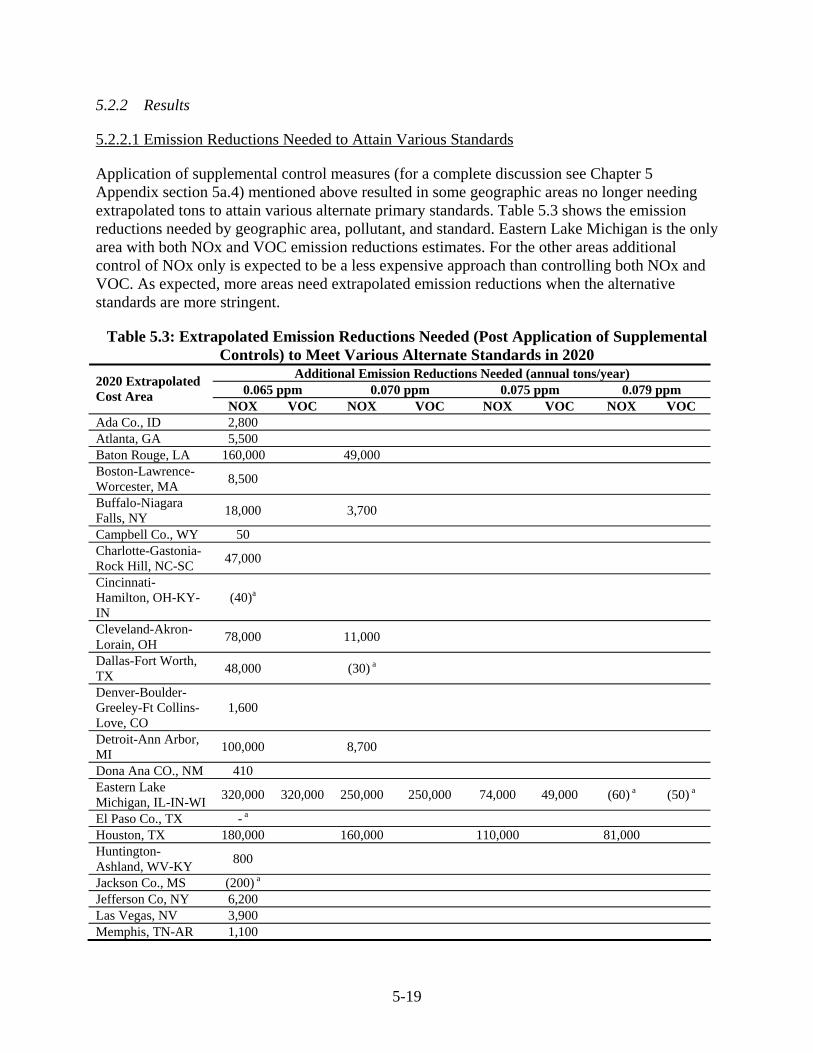
Application of supplemental control measures (for a complete discussion see Chapter 5 Appendix section 5a.4) mentioned above resulted in some geographic areas no longer needing extrapolated tons to attain various alternate primary standards. Table 5.3 shows the emission reductions needed by geographic area, pollutant, and standard. Eastern Lake Michigan is the only area with both NOx and VOC emission reductions estimates. For the other areas additional control of NOx only is expected to be a less expensive approach than controlling both NOx and VOC. As expected, more areas need extrapolated emission reductions when the alternative standards are more stringent.
Table 5.3: Extrapolated Emission Reductions Needed (Post Application of Supplemental Controls) to Meet Various Alternate Standards in 2020
Additional Emission Reductions Needed (annual tons/year) 0.065 ppm 0.070 ppm 0.075 ppm 0.079 ppm 2020 Extrapolated
Cost Area NOX VOC NOX VOC NOX VOC NOX VOC
Ada Co., ID 2,800 Atlanta, GA 5,500 Baton Rouge, LA 160,000 49,000 Boston-Lawrence-Worcester, MA 8,500
Buffalo-Niagara Falls, NY 18,000 3,700
Campbell Co., WY 50 Charlotte-Gastonia-Rock Hill, NC-SC 47,000
Cincinnati-Hamilton, OH-KY-IN
(40)a
Cleveland-Akron-Lorain, OH 78,000 11,000
Dallas-Fort Worth, TX 48,000 (30) a
Denver-Boulder-Greeley-Ft Collins-Love, CO
1,600
Detroit-Ann Arbor, MI 100,000 8,700
Dona Ana CO., NM 410 Eastern Lake Michigan, IL-IN-WI 320,000 320,000 250,000 250,000 74,000 49,000 (60) a (50) a
El Paso Co., TX - a Houston, TX 180,000 160,000 110,000 81,000 Huntington-Ashland, WV-KY 800
Jackson Co., MS (200) a Jefferson Co, NY 6,200 Las Vegas, NV 3,900 Memphis, TN-AR 1,100

5-20
Additional Emission Reductions Needed (annual tons/year) 0.065 ppm 0.070 ppm 0.075 ppm 0.079 ppm 2020 Extrapolated
Cost Area NOX VOC NOX VOC NOX VOC NOX VOC
Norfolk-Virginia Beach-Newport News
21,000
Northeast Corridor, CT-DE-MD-NJ-NY-PA
340,000 220,000 65,000
Phoenix-Mesa, AZ (60) a Pittsburgh-Beaver Valley, PA 13,000
Richmond-Petersburg, VA (600) a
Sacramento Metro, CA b 130,000 89,000 44,000 1,800
Salt Lake City, UT 430 San Juan Co., NM 1,300 St Louis, MO-IL 17,000 Toledo, OH (90) a a negative or zero values indicate the supplemental measures applied yielded equal or greater emission
reductions than were needed for the geographic area to attain the standard being analyzed. b Sacramento Metro, CA geographic area also contains the South Coast and San Joaquin Valley Areas.
These two areas will still be reducing emissions to meet the 0.08 ozone standard, and therefore the costs of these emission reductions are not incurred as part of meeting a new ozone standard. The difference between the emission reductions needed in Table 4.7a and this table are accounted for by the tons that South Coast and San Joaquin need to reduce to reach the current standard, and to help Sacramento attain a new ozone standard.
5.2.2.2 Fixed Cost Approach Extrapolated Costs
Figure 5.6 and Table 5.4 presents the extrapolated cost estimates regionally for the various alternative standards for a fixed cost approach of $15,000/ton. These costs are the values from Table 5.3 multiplied by $15,000. See the Appendix 5a.4.3 for sensitivity analyses of varying the fixed dollar per ton to values other than $15,000. When we evaluate the portion of costs for the extrapolated costs fixed approach by supplemental air quality modeling phase (as described in Chapter 4), 100% of the costs are allocated to phase 1 geographic areas for the 0.075 ppm and 0.079 ppm standard. For the 0.065 ppm and 0.070 ppm standards 73% to 94% are allocated to phase 1 areas, 22% to 6% in phase 2 areas, and only 5% to 0% for phase 3 areas. The sensitivity analysis for the fixed cost approach at $10,000/ton and $20,000/ton resulted in extrapolated costs of $3.4 to $6.8 billion dollars for the 0.075 ppm standard.
5.2.2.3 Hybrid Approach Extrapolated Cost Results
Table 5.5 presents the extrapolated cost estimates regionally for the various alternative standards for the hybrid approach (mid). See the Appendix 5a.4.4 for sensitivity analyses of values of M of 0.47 and 0.12. A value of 0.24 is used for M because R goes up with the stringency of the standard, the differences in costs between cost areas increase with the stringency of the

5-21
Figure 5.6: Extrapolated Cost by Region to Meet Various Alternate Standards Using Fixed Cost Approach ($15,000/ton)
0.065 ppm0.070 ppm
0.075 ppm0.079 ppm
CA
West
East
$0
$5
$10
$15
$20
$25
$30
$35
$40
Extr
apol
ated
Cos
t (B
200
6$)
Table 5.4: Extrapolated Cost by Region to Meet Various Alternate Standards Using Fixed Cost Approach ($15,000/ton) a, b
Fixed Cost Approach Extrapolated Cost (M 2006$) 2020 Extrapolated Cost by Region 0.065 ppm 0.070 ppm 0.075 ppm 0.079 ppm
East $25,000 $14,000 $4,500 $1,200 West $160 - - - California $2,000 $1,300 $660 $28 Total Extrapolated Cost $27,000 $16,000 $5,100 $1,200 a All estimates rounded to two significant figures. As such, totals will not sum down columns. b These estimates do not reflect benefits or costs for the San Joaquin Valley or South Coast Air Basins.
Please see Appendix 7b for analysis of these areas.
alternative being considered. When we evaluate the portion of costs for the extrapolated costs fixed approach by supplemental air quality modeling phase (as described in Chapter 4), 100% of the costs are allocated to phase 1 geographic areas for the 0.075 ppm and 0.079 ppm standard. For the 0.065 ppm and 0.070 ppm standards 74% to 95% are allocated to phase 1 areas, 21% to 5% in phase 2 areas, and only 5% to 0% for phase 3 areas.

5-22
Figure 5.7: Extrapolated Cost by Region to Meet Various Alternate Standards Using Hybrid Approach (Mid)
0.065 ppm0.070 ppm
0.075 ppm0.079 ppm
CA
West
East
$0
$5
$10
$15
$20
$25
$30
$35
$40
Extr
apol
ated
Cos
t (B
200
6$)
Table 5.5: Extrapolated Cost by Region to Meet Various Alternate Standards Using Hybrid Approach (Mid) a, b
Hybrid Approach Extrapolated Cost (M 2006$) 2020 Extrapolated Cost by Region 0.065 ppm 0.070 ppm 0.075 ppm 0.079 ppm
East $36,000 $20,000 $5,500 $1,700 West $170 California $2,800 $1,700 $770 $28 Total Extrapolated Cost $39,000 $22,000 $6,300 $1,800 a All estimates rounded to two significant figures. As such, totals will not sum down columns. b These estimates do not reflect benefits or costs for the San Joaquin Valley or South Coast Air Basins.
Please see Appendix 7b for analysis of these areas.
5-23
5.3 Summary of Costs
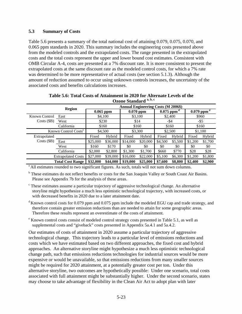
Table 5.6 presents a summary of the total national cost of attaining 0.079, 0.075, 0.070, and 0.065 ppm standards in 2020. This summary includes the engineering costs presented above from the modeled controls and the extrapolated costs. The range presented in the extrapolated costs and the total costs represent the upper and lower bound cost estimates. Consistent with OMB Circular A-4, costs are presented at a 7% discount rate. It is more consistent to present the extrapolated costs at the same discount rate as the modeled control costs, for which a 7% rate was determined to be more representative of actual costs (see section 5.1.3). Although the amount of reduction assumed to occur using unknown controls increases, the uncertainty of the associated costs and benefits calculations increases.
Table 5.6: Total Costs of Attainment in 2020 for Alternate Levels of the Ozone Standard a, b, c
Annual Engineering Costs (M 2006$) Region 0.065 ppm 0.070 ppm 0.075 ppm d 0.079 ppm d
East $4,100 $3,100 $2,400 $960 West $230 $14 -$4 -$5
Known Control Costs ($B)
California $160 $160 $160 $160 Known Control Costse $4,500 $3,300 $2,500 $1,100
Fixed Hybrid Fixed Hybrid Fixed Hybrid Fixed Hybrid East $25,000 $36,000 $14,000 $20,000 $4,500 $5,500 $1,200 $1,700 West $160 $170 $0 $0 $0 $0 $0 $0
Extrapolated Costs ($B)
California $2,000 $2,800 $1,300 $1,700 $660 $770 $28 $28 Extrapolated Costs $27,000 $39,000 $16,000 $22,000 $5,100 $6,300 $1,200 $1,800 Total Cost Range $32,000 $44,000 $19,000 $25,000 $7,600 $8,800 $2,400 $2,900
a All estimates rounded to two significant figures. As such, totals will not sum down columns. b These estimates do not reflect benefits or costs for the San Joaquin Valley or South Coast Air Basins.
Please see Appendix 7b for the analysis of these areas. c These estimates assume a particular trajectory of aggressive technological change. An alternative
storyline might hypothesize a much less optimistic technological trajectory, with increased costs, or with decreased benefits in 2020 due to a later attainment date.
d Known control costs for 0.079 ppm and 0.075 ppm include the modeled EGU cap and trade strategy, and therefore contain greater emission reductions than are needed to attain for some geographic areas. Therefore these results represent an overestimate of the costs of attainment.
e Known control costs consist of modeled control strategy costs presented in Table 5.1, as well as supplemental costs and “giveback” costs presented in Appendix 5a.4.1 and 5a.4.2.
Our estimates of costs of attainment in 2020 assume a particular trajectory of aggressive technological change. This trajectory leads to a particular level of emissions reductions and costs which we have estimated based on two different approaches, the fixed cost and hybrid approaches. An alternative storyline might hypothesize a much less optimistic technological change path, such that emissions reductions technologies for industrial sources would be more expensive or would be unavailable, so that emissions reductions from many smaller sources might be required for 2020 attainment, at a potentially greater cost per ton. Under this alternative storyline, two outcomes are hypothetically possible: Under one scenario, total costs associated with full attainment might be substantially higher. Under the second scenario, states may choose to take advantage of flexibility in the Clean Air Act to adopt plan with later

5-24
attainment dates to allow for additional technologies to be developed and for existing programs like EPA’s Onroad Diesel, CAIR, Nonroad Diesel, and Locomotive and Marine rules to be fully implemented. If states were to submit plans with attainment dates beyond our 2020 analysis year, benefits would clearly be lower than we have estimated under our analytical storyline. However, in this case, state decision makers, seeking to maximize economic efficiency, would not impose costs, including potential opportunity costs of not meeting their attainment date, when they exceed the expected health benefits that states would realize from meeting their modeled 2020 attainment date. In this case, upper bound costs are difficult to estimate because we do not have an estimate of the point where marginal costs are equal to marginal benefits plus the costs of nonattainment.
Figure 5.8 shows the total costs for both the fixed and hybrid approaches broken out by region.
Figure 5.8: Annual Total Costs by Regiona
$0
$5
$10
$15
$20
$25
$30
$35
$40
$45
Tota
l Cos
t (B
200
6$)
0.065
ppm
0.070
ppm
0.075
ppm
0.079
ppm
0.065
ppm
0.070
ppm
0.075
ppm
0.079
ppm
Total Cost - Fixed ($15,000/ton) Total Cost - Hybrid (Mid)
West CA East
a These estimates assume a particular trajectory of aggressive technological change. An alternative storyline might hypothesize a much less optimistic technological trajectory, with increased costs, or with decreased benefits in 2020 due to a later attainment date.
Figure 5.9 separates the total cost under both the fixed and extrapolated cost approaches into the known control costs and the extrapolated costs. This shows graphically the increasing portion of costs that comes from unknown controls as the standard tightens. Depending upon the standard and extrapolated cost methodology (fixed or hybrid) the costs from unknown control technologies ranges from 50% to 89% of the total costs.

5-25
Figure 5.9: National Known Control Costs and Extrapolated Costs for Various Standardsa, b
$0
$5
$10
$15
$20
$25
$30
$35
$40
$45To
tal C
osts
(B 2
006$
)
0.065
ppm
0.070
ppm
0.075
ppm
0.079
ppm
0.065
ppm
0.070
ppm
0.075
ppm
0.079
ppm
Total Cost ($15,000/ton) Total Cost (Mid)
Known Control Costs Fixed Extrapolated Cost ($15,000/ton) Hybrid Extrapolated Cost (Mid)
a Known control costs consist of modeled control strategy costs presented in Table 5.1, as well as supplemental costs and “giveback” costs presented in Appendix 5a.4.1 and 5a.4.2.
c These estimates assume a particular trajectory of aggressive technological change. An alternative storyline might hypothesize a much less optimistic technological trajectory, with increased costs, or with decreased benefits in 2020 due to a later attainment date.
Lastly, Figure 5.10 shows the total cost range by standard. For the final standard of 0.075 ppm the total cost ranges from $7.6 to $8.8 billion.

5-26
Figure 5.10: Total Cost Ranges for Various Standardsa
$0
$5
$10
$15
$20
$25
$30
$35
$40
$45
Tota
l Ann
ual C
osts
(B 2
006$
)
0.065 ppm 0.070 ppm 0.075 ppm 0.079 ppm
Total Cost - Fixed ($15,000/ton) Total Cost - Hybrid (Mid) a These estimates assume a particular trajectory of aggressive technological change. An alternative
storyline might hypothesize a much less optimistic technological trajectory, with increased costs, or with decreased benefits in 2020 due to a later attainment date.
5.4 Technology Innovation and Regulatory Cost Estimates
There are many examples in which technological innovation and “learning by doing” have made it possible to achieve greater emissions reductions than had been feasible earlier, or have reduced the costs of emission control in relation to original estimates. Studies10 have suggested that costs of some EPA programs have been less than originally estimated due in part to inadequate inability to predict and account for future technological innovation in regulatory impact analyses.
Technological change will affect baseline conditions for our analysis. This change may lead to potential improvements in the efficiency with which firms produce goods and services, for example, firms may use less energy to produce the same quantities of output. In addition, technological change may result in improvements in the quality of health care, which can have impacts on the baseline health of the population, potentially reducing the susceptibility of the population to the effects of air pollution. While our baseline mortality incidence rates account for
10 Harrington et al. (2000) and previous studies cited by Harrington.

5-27
increasing life expectancy, and thus reflect projected improvements in health care, our baseline incidence rates for other health endpoints such as hospital admissions do not reflect any future
advances in health care, and thus, our estimates of avoided health impacts for these endpoints will potentially be overstated. For other endpoints, such as asthma, there has been an observed upward trend in prevalence, which we have not captured in our incidence rates. For these endpoints, our estimates will potentially be understated. In general, for non-mortality endpoints, there is increased uncertainty in our estimates due to our use of current baseline incidence and prevalence rates.
Constantly increasing marginal costs are likely to induce the type of innovation that would result in lower costs than estimated early in this chapter. Breakthrough technologies in control equipment could by 2020 result in a rightward shift in the marginal cost curve for such equipment (Figure 5.11)11 as well as perhaps a decrease in its slope, reducing marginal costs per unit of abatement, and thus deviate from the assumption of one constantly increasing marginal cost curve. In addition, elevated abatement costs may result in significant increases in the cost of production and would likely induce production efficiencies, in particular those related to energy inputs, which would lower emissions from the production side.
Figure 5.11: Technological Innovation Reflected by Marginal Cost Shift
MC0 MC1
Cumulative NOx Reductions
Cos
t/Ton
Induced Technology Shift
Slope = β 0
Slope = β 1
5.4.1 Examples of Technological Advances in Pollution Control
There are numerous examples of low-emission technologies developed and/or commercialized over the past 15 or 20 years, such as:
• Selective catalytic reduction (SCR) and ultra-low NOx burners for NOx emissions
11 Figure 5.2 shows a linear marginal abatement cost curve. It is possible that the shape of the marginal abatement cost curve is non-linear.

5-28
• Scrubbers which achieve 95% and even greater SO2 control on boilers
• Sophisticated new valve seals and leak detection equipment for refineries and chemical plans
• Low or zero VOC paints, consumer products and cleaning processes
• Chlorofluorocarbon (CFC) free air conditioners, refrigerators, and solvents
• Water and powder-based coatings to replace petroleum-based formulations
• Vehicles far cleaner than believed possible in the late 1980s due to improvements in evaporative controls, catalyst design and fuel control systems for light-duty vehicles; and treatment devices and retrofit technologies for heavy-duty engines
• Idle-reduction technologies for engines, including truck stop electrification efforts
• Market penetration of gas-electric hybrid vehicles, and clean fuels
These technologies were not commercially available two decades ago, and some were not even in existence. Yet today, all of these technologies are on the market, and many are widely employed. Several are key components of major pollution control programs.
What is known as “learning by doing” or “learning curve impacts” have also made it possible to achieve greater emissions reductions than had been feasible earlier, or have reduced the costs of emission control in relation to original estimates. Learning curve impacts can be defined generally as the extent to which variable costs (of production and/or pollution control) decline as firms gain experience with a specific technology. Such impacts have been identified to occur in a number of studies conducted for various production processes. Impacts such as these would manifest themselves as a lowering of expected costs for operation of technologies in the future below what they may have been.
The magnitude of learning curve impacts on pollution control costs has been estimated for a variety of sectors as part of the cost analyses done for the Draft Direct Cost Report for the second EPA Section 812 Prospective Analysis of the Clean Air Act Amendments of 1990.12 In that report, learning curve adjustments were included for those sectors and technologies for which learning curve data was available. A typical learning curve adjustment example is to reduce either capital or O&M costs by a certain percentage given a doubling of output from that sector or for that technology. In other words, capital or O&M costs will be reduced by some percentage for every doubling of output for the given sector or technology.
12 E.H. Pechan and Associates and Industrial Economics, Direct Cost Estimates for the Clean Air Act Second Section 812 Prospective Analysis: Draft Report, prepared for U.S. EPA, Office of Air and Radiation, February 2007. Available at http://www.epa.gov/oar/sect812/mar07/direct_cost_draft.pdf.
5-29
T.P. Wright, in 1936, was the first to characterize the relationship between increased productivity and cumulative production. He analyzed man-hours required to assemble successive airplane bodies. He suggested the relationship is a log linear function, since he observed a constant linear reduction in man-hours every time the total number of airplanes assembled was doubled. The relationship he devised between number assembled and assembly time is called Wright’s Equation (Gumerman and Marnay, 2004).13 This equation, shown below, has been shown to be widely applicable in manufacturing:
Wright’s Equation: CN = Co * Nb,
where
N = cumulative production
CN = cost to produce Nth unit of capacity
Co = cost to produce the first unit
B = learning parameter = ln (1-LR)/ln(2), where
LR = learning by doing rate, or cost reduction per doubling of capacity or output.
The percentage adjustments can range from 5 to 20 percent, depending on the sector and technology. Learning curve adjustments were prepared in a memo by IEc (2007) supplied to US EPA and applied for the mobile source sector (both onroad and nonroad) and for application of various EGU control technologies within the Draft Direct Cost Report.14 Advice received from the SAB Advisory Council on Clean Air Compliance Analysis in June 2007 indicated an interest in expanding the treatment of learning curves to those portions of the cost analysis for which no learning curve impact data are currently available. Examples of these sectors are non-EGU point sources and area sources. The memo by IEc outlined various approaches by which learning curve impacts can be addressed for those sectors. The recommended learning curve impact adjustment for virtually every sector considered in the Draft Direct Cost Report is a 10% reduction in O&M costs for two doubling of cumulative output, with proxies such as cumulative fuel sales or cumulative emission reductions being used when output data was unavailable.
For this RIA, we do not have the necessary data for cumulative output, fuel sales, or emission reductions for sectors included in our analysis in order to properly generate control costs that reflect learning curve impacts. Clearly, the effect of including these impacts would be to lower
13 Gumerman, Etan and Marnay, Chris. Learning and Cost Reductions for Generating Technologies in the National Energy Modeling System (NEMS), Ernest Orlando Lawrence Berkeley National Laboratory, University of California at Berkeley, Berkeley, CA. January 2004, LBNL-52559. 14 Industrial Economics, Inc. Proposed Approach for Expanding the Treatment of Learning Curve Impacts for the Second Section 812 Prospective Analysis: Memorandum, prepared for U.S. EPA, Office of Air and Radiation, August 13, 2007.

5-30
our estimates of costs for our control strategies in 2020, but we are not able to include such an analysis in this RIA.
5.4.2 Influence on Regulatory Cost Estimates
Studies indicate that it is not uncommon for pre-regulatory cost estimates to be higher than later estimates, in part because of inability to predict technological advances. Over longer time horizons, such as the time allowed for areas with high levels of ozone pollution to meet the ozone NAAQS, the opportunity for technical advances is greater.
• Multi-rule study: Harrington et al. of Resources for the Future (2000) conducted an analysis of the predicted and actual costs of 28 federal and state rules, including 21 issued by EPA and the Occupational Safety and Health Administration (OSHA), and found a tendency for predicted costs to overstate actual implementation costs. Costs were considered accurate if they fell within the analysis error bounds or if they fall within 25 percent (greater or less than) the predicted amount. They found that predicted total costs were overestimated for 14 of the 28 rules, while total costs were underestimated for only three rules. Differences can result because of quantity differences (e.g., overestimate of pollution reductions) or differences in per-unit costs (e.g., cost per unit of pollution reduction). Per-unit costs of regulations were overestimated in 14 cases, while they were underestimated in six cases. In the case of EPA rules, the agency overestimated per-unit costs for five regulations, underestimated them for four regulations (three of these were relatively small pesticide rules), and accurately estimated them for four. Based on examination of eight economic incentive rules, “for those rules that employed economic incentive mechanisms, overestimation of per-unit costs seems to be the norm,” the study said.
Based on the case study results and existing literature, the authors identified technological innovation as one of five explanations of why predicted and actual regulatory cost estimates differ: “Most regulatory cost estimates ignore the possibility of technological innovation … Technical change is, after all, notoriously difficult to forecast … In numerous case studies actual compliance costs are lower than predicted because of unanticipated use of new technology.”15
It should be noted that many (though not all) of the EPA rules examined by Harrington had compliance dates of several years, which allowed a limited period for technical innovation. Much longer time periods (ranging up to 20 years) are allowed by the statute for meeting the ozone NAAQS in areas with high ozone levels, where a substantial fraction of the estimated cost in this analysis is incurred.
• Acid Rain SO2 Trading Program: Recent cost estimates of the Acid Rain SO2 trading program by Resources for the Future (RFF) and MIT have been as much as 83 percent lower than originally projected by EPA.16 Note that the original EPA cost analysis also relied on an optimization model like IPM to approximate the results of emissions trading.
15 Harrington et al., 2000. 16 Carlson et al., 2000; Ellerman, 2003.

5-31
As noted in the RIA for the Clean Air Interstate Rule, the ex ante numbers in 1989 were an overestimate in part because of the limitation of economic modeling to predict technological improvement of pollution controls and other compliance options such as fuel switching. The fuel switching from high-sulfur to low-sulfur coal was spurred by a reduction in rail transportation costs due to deregulation of rail rates during the 1990’sHarrington et al. report that scrubbing turned out to be more efficient (95% removal vs. 80-85% removal) and more reliable (95% vs. 85% reliability) than expected, and that unanticipated opportunities arose to blend low and high sulfur coal in older boilers up to a 40/60 mixture, compared with the 5/95 mixture originally estimated.
Phase 2 Cost Estimates Ex ante estimates $2.7 to $6.2 billiona Ex post estimates $1.0 to $1.4 billion a 2010 Phase II cost estimate in $1995.
• EPA Fuel Control Rules: A 2002 study by two economists with EPA’s Office of Transportation and Air Quality17 examined EPA vehicle and fuels rules and found a general pattern that “all ex ante estimates tended to exceed actual price impacts, with the EPA estimates exceeding actual prices by the smallest amount.” The paper notes that cost is not the same as price, but suggests that a comparison nonetheless can be instructive.18 An example focusing on fuel rules is provided:
Table 5.7: Comparison of Inflation-Adjusted Estimated Costs and Actual Price Changes for EPA Fuel Control Rules A
Inflation-adjusted Cost Estimates (c/gal) EPA DOE API Other
Actual Price Changes (c/gal)
Gasoline Phase 2 RVP Control (7.8
RVP—Summer) (1995$) 1.1 1.8 0.5
Reformulated Gasoline Phase 1 (1997$)
3.1-5.1 3.4-4.1 8.2-14.0 7.4 (CRA) 2.2
Reformulated Gasoline Phase 2 (Summer) (2000$)
4.6-6.8 7.6-10.2 10.8-19.4 12 7.2 (5.1, when corrected to 5yr MTBE price)
30 ppm sulfur gasoline (Tier 2) 1.7-1.9 2.9-3.4 2.6 5.7 (NPRA), 3.1 (AIAM)
N/A
Diesel 500 ppm sulfur highway diesel
fuel (1997$) 1.9-2.4 3.3
(NPRA) 2.2
15 ppm sulfur highway diesel fuel
4.5 4.2-6.0 6.2 4.2-6.1 (NPRA)
N/A
a Anderson et al., 2002.
17 Anderson et al, 2002. 18 The paper notes: “Cost is not the same as price. This simple statement reflects the fact that a lot happens between a producer’s determination of manufacturing cost and its decisions about what the market will bear in terms of price change.”

5-32
• Chlorofluorocarbon (CFC) Phase-Out: EPA used a combination of regulatory, market based (i.e., a cap-and-trade system among manufacturers), and voluntary approaches to phase out the most harmful ozone depleting substances. This was done more efficiently than either EPA or industry originally anticipated. The phaseout for Class I substances was implemented 4-6 years faster, included 13 more chemicals, and cost 30 percent less than was predicted at the time the 1990 Clean Air Act Amendments were enacted.19
The Harrington study states, “When the original cost analysis was performed for the CFC phase-out it was not anticipated that the hydrofluorocarbon HFC-134a could be substituted for CFC-12 in refrigeration. However, as Hammit (1997) notes, ‘since 1991 most new U.S. automobile air conditioners have contained HFC-134a (a compound for which no commercial production technology was available in 1986) instead of CFC-12” (p.13). He cites a similar story for HCFRC-141b and 142b, which are currently substituting for CFC-11 in important foam-blowing applications.”
• Additional examples of decreasing costs of emissions controls include: SCR catalyst costs decreasing from $11k-$14k in 1998 to $3.5k-$5k in 2004, and improved low NOx burners reduced emissions by 50% from 1993-2003 while the associated capital cost dropped from $25-$38/kw to $15/kw (ICF, 2005).
We can not estimate the interplay between EPA regulation and technology improvement, but it is clear that a priori cost estimation often results in overestimation of costs because changes in technology (whatever the cause) make less costly control possible.
5.5 References
Anderson, J.F., and Sherwood, T., 2002. “Comparison of EPA and Other Estimates of Mobile Source Rule Costs to Actual Price Changes,” Office of Transportation and Air Quality, U.S. Environmental Protection Agency. Technical Paper published by the Society of Automotive Engineers. SAE 2002-01-1980.
Babiker, M.H., and T.F. Rutherford. 1997. “Input Output and General Equilibrium Estimates of Embodied CO2: A Data Set and Static Framework for Assessment.” University of Colorado at Boulder, Working Paper 97 2. Available at http://debreu.colorado.edu/papers/gtaptext.html.
Babiker, M.H., J.M. Reilly, M. Mayer, R.S. Eckaus, I.S. Wing, and R.C. Hyman. 2001. “The MIT Emissions Prediction and CO2 Policy Analysis (EPPA) Model: Revisions, Sensitivities, and Comparisons of Results.” MIT Joint Program on the Science and Policy of Global Change, Report No. 71. Available at http://web.mit.edu/globalchange/www/eppa.html.
Bovenberg, L.A., and L.H. Goulder. 1996. “Optimal Environmental Taxation in the Presence of Other Taxes: General Equilibrium Analysis.” American Economic Review 86(4):985-1000. Available at <http://www.aeaweb.org/aer/>.
19 Holmstead, 2002.

5-33
Brooke, A., D. Kendrick, A. Meeraus, and R. Raman. 1998. GAMS: A User’s Guide. GAMS Development Corporation. Available at http://www.gams.com.
Carlson, Curtis, Dallas R. Burtraw, Maureen, Cropper, and Karen L. Palmer. 2000. “Sulfur Dioxide Control by Electric Utilities: What Are the Gains from Trade?” Journal of Political Economy 108(#6):1292-1326.
Ellerman, Denny. January 2003. Ex Post Evaluation of Tradable Permits: The U.S. SO2 Cap-and-Trade Program. Massachusetts Institute of Technology Center for Energy and Environmental Policy Research.
Feenberg, D., and E. Coutts. 1993. “An Introduction to the TAXSIM Model.” Journal of Policy Analysis and Management 12(1):189 194. Available at http://www.nber.org/~taxsim/.
Fullerton, D., and D. Rogers. 1993. “Who Bears the Lifetime Tax Burden?” Washington, DC: The Brookings Institute. Available at http://bookstore.brookings.edu/ book_details.asp?product%5Fid=10403.
Goulder, L.H., and R.C. Williams. 2003. “The Substantial Bias from Ignoring General Equilibrium Effects in Estimating Excess Burden, and a Practical Solution.” Journal of Political Economy 111:898 927. Available at http://www.journals.uchicago.edu/JPE/home.html
Harrington, W., R.D. Morgenstern, and P. Nelson. 2000. “On the Accuracy of Regulatory Cost Estimates.” Journal of Policy Analysis and Management 19(2):297-322.
Hammit, J.K. (1997). “Are the costs of proposed environmental regulations overestimated? Evidence from the CFC phaseout.” Unpublished paper, Center for Risk Analysis, Harvard School of Public Health, Cambridge, MA.
Holmstead, Jeffrey, 2002. “Testimony of Jeffrey Holmstead, Assistant Administrator, Office of Air and Radiation, U.S. Environmental Protection Agency, Before the Subcommittee on Energy and air Quality of the committee on Energy and Commerce, U.S. House of Representatives, May 1, 2002, p. 10.
ICF Consulting. October 2005. The Clean Air Act Amendment: Spurring Innovation and Growth While Cleaning the Air. Washington, DC. Available at http://www.icfi.com/Markets/Environment/doc_files/caaa-success.pdf.
Minnesota IMPLAN Group. 2003. State Level Data for 2000. Available from http://www.implan.com/index.html.
Nestor, D.V., and C.A. Pasurka. 1995. The U.S. Environmental Protection Industry: A Proposed Framework for Assessment. U.S. Environmental Protection Agency, Office of Policy, Planning, and Evaluation. EPA 230-R-95-001. Available at http://yosemite.epa.gov/ee/epa/eermfile.nsf/11f680ff78df42f585256b45007e6235/41b8b642ab9371df852564500004b543/$FILE/EE 0217A 1.pdf.

5-34
U.S. Department of Energy, Energy Information Administration. Undated (b). State Energy Price and Expenditure Report. Washington DC. Available at http://www.eia.doe.gov/emeu/states/price_multistate.html.
U.S. Department of Energy, Energy Information Administration. 2001. Manufacturing Energy Consumption Survey 1998. Washington DC. Available at http://www.eia.doe.gov/emeu/mecs/.
U.S. Department of Energy, Energy Information Administration. January 2003. Annual Energy Outlook 2003. DOE/EIA 0383(2003). Washington DC. Available at http://www.eia.doe.gov/oiaf/archive/aeo03/pdf/0383(2003).pdf.
U.S. Department of Energy, Energy Information Administration. January 2004. Annual Energy Outlook 2004. DOE/EIA-0383(2003). Washington, DC. Available at http://www.eia.doe.gov/oiaf/aeo/pdf/0383 (2001).
U.S. Environmental Protection Agency. June 2007. Advisory Council on Clean Air Compliance Analysis (COUNCIL), Council Advisory on OAR’s Direct Cost Report and Uncertainty Analysis Plan. Washington, DC. http://www.epa.gov/sab/pdf/council-07-002.pdf.