Chapter 5 DETERMINANTS OF FDI IN INDIA: AN...
41
Chapter 5 DETERMINANTS OF FDI IN INDIA: AN ECONOMETRIC ANALYSIS The aim of this chapter is to identify the determinants of FDI inflows in vanous industries and states of India, as well as those for aggregate inflows, by employing tools of applied econometrics. We employ panel models for examining the determinants of FDI across industries and states of India. FDI inflows across industries and states over a period of time are examined in terms of various industry and state-specific explanatory variables. Accordingly, panels ofFDI inflows across industries and states are constructed. We also analyse the determinants of aggregate FDI inflows in India in terms of specific macroeconomic parameters using simple time series data. The chapter is organised into four sections. Section 1 sets up the testable hypotheses. Section 2 specifies the econometric models for estimation, discusses the data and variables and explains the econometric methodology employed. Section 3 reports and analyses the results. Section 4 gives a synthesis of the main findings. 5.1 TESTABLE HYPOTHESES We categorise our hypotheses into three groups. The first group looks at industry- specific determinants of FDI. The second group focuses on state-level characteristics. The third and final group comprises macro-level determinants of aggregate FDI flows. 106
Transcript of Chapter 5 DETERMINANTS OF FDI IN INDIA: AN...

Chapter 5
DETERMINANTS OF FDI IN INDIA: AN ECONOMETRIC
ANALYSIS
The aim of this chapter is to identify the determinants of FDI inflows in vanous
industries and states of India, as well as those for aggregate inflows, by employing tools
of applied econometrics.
We employ panel models for examining the determinants of FDI across industries and
states of India. FDI inflows across industries and states over a period of time are
examined in terms of various industry and state-specific explanatory variables.
Accordingly, panels ofFDI inflows across industries and states are constructed. We also
analyse the determinants of aggregate FDI inflows in India in terms of specific
macroeconomic parameters using simple time series data.
The chapter is organised into four sections. Section 1 sets up the testable hypotheses.
Section 2 specifies the econometric models for estimation, discusses the data and
variables and explains the econometric methodology employed. Section 3 reports and
analyses the results. Section 4 gives a synthesis of the main findings.
5.1 TESTABLE HYPOTHESES
We categorise our hypotheses into three groups. The first group looks at industry
specific determinants of FDI. The second group focuses on state-level characteristics.
The third and final group comprises macro-level determinants of aggregate FDI flows.
106

5.1.1 Industry-level hypotheses
Industry size
Among various industry-level characteristics that are likely to be significant
determinants of inward FDI, we identify the size of the industry as a crucial factor.
Larger industries have well-developed markets for final products in the host country,
along with established input suppliers and skilled labour, resulting in several external
economies of scale ( orindustry size). These industries also perhaps belong to sectors in
which the host nation enjoys comparative advantage. Accordingly, we may expect more
FDI to flow into these sectors.
Empirical research on role of industry size as a determinant of FDI has been relatively
limited. This is, because, the thrust of the empirical literature on determinants of FDI
has been largely on macro-level country-specific determinants (e.g. size of the host
country market). Industry-specific studies, however, have found evidence of industry
size being a significant and positive determinant of FDI (e.g. Morgan and Wakelin
(1999), in an empirical study of the determinants of FDI in different categories of the
U.K. food industry).
Labour intensity
Given the intrinsic features of FDI in terms of specific ownership attributes (e.g. money
capital, advanced know-how, managerial expertise, marketing skills etc.), FDI flows are
expected to be directed towards relatively capital-intensive industries for better
exploitation of these ownership advantages. We may, therefore, expect less FDI flow in
relatively labour-intensive sectors. However, it must be clarified that both theoretical
107
and empirical literature has pointed out that industries usmg skilled labour more
intensively are also likely to attract more FDI. Thus, the significance of labour-intensity
in determining FDI needs to be judged by making a clear distinction between the skilled
and unskilled components of labour.
The role of relative labour-intensity, as an industry-specific characteristic in
determining FDI, has hardly been empirically examined. There are, however, instances
of empirical studies on India focusing on factors governing entry mode choices for
foreign firms in the pre-economic reform period, which have pointed to greater
concentration ofFDI in skill-intensive industries (Kumar, 1987).
Export-orientation
Empirical studies on the causality between FDI and exports have tried to ascertain
whether FDI moves into export-oriented sectors. Studies on developing countries
identify manufacturing exports as significant and positive determinants of FDI (Narula
and Wakelin, 1995; Singh and Jun, 1995). For India, however, FDI has been found to be
more biased towards the domestic market, rather than exports, as compared to
developing economies attracting high FDI, like China (Guha and Ray, 2001).
Export-orientation of industries as a determinant of FDI should be analysed to gather
insights on the nature of FDI flows, namely, whether they are more of the 'domestic
market-oriented' variety, or of an 'export-oriented' nature.
Import-intensity
Industries with higher import-intensities indicate greater dependence on imported inputs
like raw materials, stores, capital goods, know-how etc. More import-intensive
industries are likely to attract more FDI, since foreign firms have better access to
108

imports through global production and marketing networks. In many LDCs, industries
using advanced production techniques· rely heavily on technological imports due to
unavailability of quality indigenous import substitutes. FDI is expected to respond
favourably to these industries due to the oliogopolistic advantages enjoyed by foreign
firms in form of possession of advanced technology. Empirical evidence on t~e effect of
import-intensity of industries on FDI in India is very limited. We hypothesise import
intensity to have a positive impact on FDI.
Profitability
Industries earning higher profits retain larger surpluses for future investment. Moreover,
these industries are also likely to offer greater scope to foreign firms for higher
remittances to home countries. Accordingly, we expect FDI to flow into more profitable
industries.
Advertisement-intensity
Advertisement-intensity is a common feature for industries, where development of
brand loyalties through market promotion assumes considerable significance. These
industries are characterised by product differentiations through innovations. Innovations
and their successful applications are typical attributes of multinational firms.
Advertisement-intensity, therefore, is salient to industries, where ownership advantages
of FDI acquire meaningful dimensions. FDI in India has been found to have a greater
concentration in advertising-intensive industries (Kumar, 1987). We hypothesise FDI
flows to be positively related to advertisement-intensity.
109
5 .1.2 State-level hypotheses
Market size
Both theoretical and empirical literature has identified size of the host-country market
as a key determinant of FDI flows. Large markets enable foreign firms to lower their
costs of production by exploiting scale economies. Several empirical studies indicate
market size as a significant and positive determinant of FDI for both developed and
developing countries (Horst, 1972b, Root and Ahmad, 1979; Dunning, 1980, 1998a;
Schneider and Fray, 1985; Wheeler & Mody, 1992; Tsai, 1994; Taylor, 2000;
Chakraborti, 2001 ). Similar conclusions have been reached for India as well (Anand and
Delios, 1996, Guha and Ray, 2001). We propose to examine the effect of market sizes
of states on FDI flows in this study. We expect states with larger markets to attract
greater FDI.
Infrastructure
Availability of quality infrastructure facilities (e.g. rail and road transport, electricity
and telecommunication) plays an important role in attracting FDI flows. Well
developed physical and communication infrastructure helps in efficient distribution of
goods and services by lowering transaction costs. The issue of infrastructure is
particularly significant for low-income countries, which often lack in infrastructural
facilities.
Empirical studies have identified availability of infrastructure as a significant
determinant for FDI in developing countries (Wheeler & Mody, 1992; Collier, 1998,
Urata and Kawai, 1999). Shortage of quality infrastructure services has been identified
as a deterrent to FDI flows for India as well (Sachs and Bajpai, 2001), compared to
110
China and other developing economies. We hypothesise that states with better
infrastructural facilities will attract more FDI. We will also try to ascertain the
significance of transport, electricity, and telecommunication, separately, for FDI
inflows.
Industrial relations
The quality of industrial relations, reflected in the number of workdays lost, has been
found to be a significant determinant of FDI flows for developing countries receiving
low FDI (Rana, 1988; Lucas, 1993; Singh and Jun, 1995). Better industrial relations
assure foreign investors about regular participation of labour in production, apart from
indicating fewer disruptions in production schedules. We expect states with better
industrial relations to attract more FDI.
Degree of industrialisation
Ownership advantages of FDI can be exploited more meaningfully in manufacturing
and service sectors. More industrialised locations have larger presence of manufacturing
and service activities. These locations also offer a more enabling environment for FDI.
Accordingly, we hypothesise that FDI will show a higher propensity to flow into the
states that are more industrialised.
Technological capabilities and infrastructure
R&D initiatives undertaken at the state-level reflect the quality of technological
infrastructure available in the states. Higher R&D initiatives not only improve the
quality of existing technological infrastructure, but also enhance technological
capabilities. These are expected to act as 'pull' factors for FDI, since availability of
indigenous technological capabilities can help foreign firms in exploiting their
111

ownership advantages better. We hypothesise FDI flows to be positively related to the
level of technological capability and infrastructure of the states.
5.1.3 Macro-level hypotheses
Market size
We have already discussed the importance of host country market size as a determinant
for incoming FDI. Earlier, in chapter 3, we have mentioned various empirical studies
that have identified market size as a significant factor influencing FDI flows for
developed countries, LDCs, as well as the Indian economy. In the present study, we
would like to study the effect of the domestic market size on aggregate FDI inflows into
India. We expect FDI to be positively related to the size of the domestic market.
Returns to Capital
We attempt to study three related determinants ·in this category. These are stock market
returns, FII investment and non-resident deposits.
Stock market returns
Higher returns from domestic stock markets indicate higher returns on the equity capital
invested in the host economy. Though returns from stock markets are not considered
traditional determinants of FDI, neo-classical trade theory identifies differences in rates
of return as the main reason behind movement of capital across nations. In that sense,
stock market returns may reflect the incentive for capital movement. We would like to
study the impact of returns from stock markets on incoming FDI. We expect stock
market returns to have a positive relationship with FDI flows.
112
FII inflows
FII inflows into a host economy are intricately linked to returns from stock markets.
Portfolio investments by Fils are determined on the basis of their perceptions regarding
risks and returns from the host economy. These inflows usually increase if the risk··
return expectations are favourable. Higher FII inflows, reflecting positive expectations
about returns from the host economy, can encourage FDI flows. Accordingly, we
hypothesise FDI flows to be positively related to FII inflows.
Inflows of non-resident bank deposits
Bank deposits by expatriates respond favourably to the difference in interest rates
between source and host countries. Host country deposit rates reflect the nature of
returns to capital in that country. Higher inflows of non-resident deposits in response to
higher deposit rates (i.e. higher returns on capital) can motivate FDI flows, according to
the principle of capital arbitrage. We expect FDI flows to be positively related to
inflows of non-resident deposits.
( Export-orientation
Greater export-orientation of the host economy is expected to attract more FDI of the
'export-oriented' variety (Singh and Jun, 1995), Studies on India, however, suggest
greater inflow ofFDI ofthe 'domestic market-oriented' variety, rather than the 'export
oriented' type (Guha and Ray, 2001). We would like to revisit the issue in the present
study.
113

5.2 ECONOMETRIC MODEL SPECIFICATION, DATA AND VARIABLES,
AND ECONOMETRIC METHODOLOGY
5.2.1 Econometric model specification
We specify econometric models for testing our three sets of hypotheses.
Industry and state-level hypotheses
For industry and state-level hypotheses, we posit the following panel regression model:
(1) i=l,2, ....... N; t=l,2, ...... T; where
yit: FDI inflow in i-th industry in period 't'(or in i-th state in period 't').
xit: Vector of specific characteristics for i-th industry in period 't' (or i-th state in
period 't').
a1: the individual effect for the ith industry (or state) assumed to be constant
over time.
Eit : the stochastic error term.
Macro-level hypotheses
We propose a simple time series model for our macro-level analysis.
Yt= a+ f3xt + Et; (2) t=l,2, ...... T;,where
Yt : Aggregate FDI inflow in period t .
x1 : Vector of specific macro-economic parameters for period t.
E 1 : the stochastic error terriL
5.2.2 Data and variables
Our study employs panel models for identifying the determinants of FDI at the industry,
state and country levels. The variables are constructed accordingly.
114
5.2.2.1 Dependent variable (FDI)
We use actual FDI inflows as the dependent variable for testing our industry-level
hypothese~. Data on annual FDI inflows on an industry-wise basis are compiled by the
Secretariat for Industrial Assistance (SIA), Department of Industrial Promotion and
Policy, Ministry of Industry, Government of India. FDI data has been obtained from
annual issues of the SIA newsletters (2000 and 2002).
Unlike industry, data on actual FDI inflows on a state-wise basis, however, are not
available before the year 2000. Due to this data constraint, we proxy actual FDI inflows
by approved FDI flows. Approvals indicate investment intentions of foreign investors.
These intentions are influenced by the various state-level characteristics that we have
hypothesised. Accordingly, we expect results obtained by using FDI approvals to reflect
accurately the nature of relationship between incoming FDI and various explanatory
variables. Data on FDI approvals is also maintained by the SIA and was obtained from
the same sources mentioned above.
We take aggregate FDI inflows as the dependent variable for our country-level analysis.
Information on aggregate FDI inflows into India is available with both the SIA and the
RBI. On the present occasion, we use the RBI data. 38
5.2.2.2 Explanatory variables
5.2.2.2a Industry-level analysis
Industry size
We employ three variables for capturing industry size. The first of these is share of sales
of a particular industry in total industrial sales (salesxsales) for a given year.
38 See RBI (2002).
115

salesxsa/esu = (Sales of i-th industry in year 't') I Total industrial sales in year
't'.
Industry size is also measured by Sales, which reflects the value of total sales for
industry 'i' in year 't'.
The third variable used for industry size is GV AXGVA, which is the share of Gross
Value Added (GVA) by industry 'i' in year 't" in total industry GVA for year 't'.
GVAxGVAu = (GV A for i-th industry in year't')l Total industrial GV A in year
't'.
The data for industry-wise sales39 and GV A 40 have been obtained from the Corporate
Sector (May 2002) report brought out by the Centre for Monitoring Indian Economy
(CMIE).
Labour intensity
We measure labour-intensity of an industry by the share of wages and salaries of a
particular industry, i.e. the total wage bill, in industrial GV A. The variable is expressed
as wsxGVA, where,
wsxGVAit =(Wages and salaries for i-th industry in year 't') I (Total GVA fori-
th industry in year 't')
This variable fails to make a distinction between skilled and unskilled labour intensity.
Due to Jack of disaggregated data on wages and salaries for skilled and unskilled labour,
our variable reflects labour-intensity as a whole. The result, therefore, may be distorted
39 Sales are defined as Income generated from main business activities like sale of goods and services, fiscal benefits, trading income. It also includes internal transfers but excludes expenses capitalized. See CMIE (2002).
116

in reporting the essence of the labour-intensity hypothesis. We_would like to clarify that
though we expect FDI to flow more into capital-intensive industries, given the
significance of skilled labour as a determinant of FDI, we should ideally employ
variables that measure labour-intensities separately in terms of skilled and unskilled
components.
Data on wages and salaries have been taken from the CMIE data source cited earlier.
Export-orientation
Export-orientation is measured by the volume of exports from a particular industry as a
proportion of total industrial sales. The variable is expressed as expxsales, where
expxsalesit = (Total export earnings41 for i-th industry in year 't') I (Total sales
for i-th industry in year 't')
Data on export earnings and industrial sales have been obtained from the CMIE data
source.
Import-intensitv
We measure import-intensity by the volume of imports for an industry as a proportion
of total industrial sales. The variable is expressed as impxsales, where
impxsalesit = (Total import expenses42 for i-th industry in year 't') I (Total sales
for i-th industry in year 't')
Data for import earnings have been taken from the CMIE data source.
40 GV A is defmed as the sum of wages and salaries, interest payments, rent paid, profit before tax, and depreciation. Interest and rent payments are net of receipts, while profit before tax is net of non-recurring transactions. See CMIE (2002) 41 Total exports are defined as total forex earnings, including earnings from export of goods on FOB value, as well as forex earnings from services. See CMIE (2002).
117

Profitability
Profitability of industries is measured by the share of profit after tax (PAT) (net of non-
recurring transactions) in total sales of an industry. The variable is expressed as
pat.xsales, where,
Pat.xsalesit = (Total profits after tax for i-th industry in year 't') I (Total sales for
i-th industry in year 't')
Data on profit after tax has been taken from CMIE.
Advertisement-intensitv
We use the share of advertising expenses, as a proportion of total industrial sales, as a
measure of advertisement-intensity. The variable is expressed as advtxsales, where
advtxsalesit = (Total advertising expenditure for i-th industry in year 't') /
(Total sales for i-th industry in year 't')
Data on advertising expenses43 has also been collected from the CMIE.
A note on the CMIE data source is given in Appendix 1.
For the industry-level analysis, we estimate the panel regression model specified in the
earlier section for two different data sets. The first data set comprises eighteen
manufacturing industries. These are: metallurgical, fuels, electrical equipment,
transportation, non-electrical machinery, fertilizers, chemicals, drugs &
phmmaceuticals, textiles, paper; sugar, fermentation, food processing, vegetable oi1s,
rubber, soaps & cosmetics, leather and cement.
42 Total import expenses include the CIF value of import of raw materials, stores, import of capital goods and also foreign exchange outgo on royalty, know-how, fees, dividend, interest etc. See CMIE (2002). 43 Advertising cost is defmed as the expenditure incurred on advertising. It also includes marketing expenditure such as rebates, discounts and commissions. See CMIE (2002).
118
The second data set includes services, hotel & tourism, and trading, in addition to the
eighteen manufacturing industries. However, due to lack of data on advertising cost for
services, we had to drop advtxls as an explanatory variable from the second variation.
The time period for estimation is 1994-95 to2000-01.
5.2.2.2b State-level analysis
Market size
We capture the size of domestic market for states through annual per capita net state
domestic product (SDP) at current prices. The variable is expressed as pcnsdp. Per
capita net SDP is an income proxy of the market size, reflecting the purchasing power.
Market size can also be measured in terms of the absolute value of net SDP. However,
we have constructed pcnsdp after normalising absolute values ofNSDP by population.
Values of pcnsdp have been obtained from the annual Economic Survey (2002-03)
published by the Ministry of Finance, Government of India.
Infrastructure
In our analysis, we focus specifically upon three major components of infrastructure.
These are transport infrastructure, electricity, and telecommunication, respectively. We
measure transport infrastructure through two variables: raildensity and rddensity. While
raildensity indicates the state-wise density of rail route length per '000 sq. km. of area,
rddensity is state-wise density of road length per '000 sq. km. of geographical area.
Data for both these variables have been obtained from the Infrastructure report44
brought out by the CMIE.
44 See CMIE (2003).
119

We measure availability of electricity through per capita electricity consumption in
states. The variable is expressed as pcelecon. Data on state-level per capita electricity
consumption has been taken from the Annual Report (2001-02) on the Working of State.
Electricity Boards & Electricity Departments brought out by the Planning Commission.
Finally, we try to capture the availability of telecommunication services by delciricle,
which measures circle-wise direct exchange lines (provided by BSNL & MTNL) in
'000 numbers for every state. Data on number of circle-wise direct exchange lines has
also been obtained from the CMIE database cited above.
Quality of industrial relations
Quality of industrial relations in various states is measured by number of mandays lost
on account of strikes and lockouts. The variable is expressed as mtmdays. Information
on number of mandays lost annually, state-wise, has been obtained from various issues
of the Handbook of Indhstrial Statistics published by the Department of Industrial
Promotion & Policy (DIP&P), Government oflndia.
Degree of industrialisation
We use the share of non-agricultural domestic product in net SDP at current prices, as a
measure for degree of industrialisation. The variable is expressed as nonagrdp.
nonagrdpit = 1- (Net domestic product from agriculture in i-th state in year
't')/(Total net domestic product in i-th state in year 't')
Values of nonagrdp for different states have been calculated on the basis of sectoral and
aggregate estimates for SDPs from the National Accounts Statistics compiled by the
Central Statistical Organisation (CSO).
120
Technological Capabilities and Infrastructure
We have tried to quantify the level of technological capabilities and infrastructure at
state-level in terms of share of R&D expenditure as a proportion of per capita net SDP
for each state. The variable is expressed as rdpcnsdp.
rdpcnsdpu = (Total R&D expenditure by state 'i' m year 't') I (Per capita
NSDP for state 'i' in year 't')
The values of rdpcnsdp has been estimated on the basis of data on state-level R&D
expenditure, compiled from statistics released by the Department of Science and
Technology in various issues of the Handbook of Industrial Statistics brought out by the
Ministry of Industry, Government of India.
The panel regression model specified in the earlier section has been estimated for
sixteen states of the country. These are: Andhra Pradesh, Assam, Bihar,, Gujarat,
Haryana, Himachal Pradesh, Karnataka, Kerala, Madhya Pradesh, Maharashtra, Orissa,
Punjab, Rajasthan, Tamilnadu, Uttar Pradesh and West Bengal.
Due to lack of data for one or more of the explanatory variables, other states and Union
Territories could not be included. The sixteen states figuring in our estimation account
for more than eighty per cent of total FDI approvals during the 'period 1993-94 to 2000-
01. Among the states excluded, only Delhi has sizeable FDI approvals. However, we
could not include Delhi due to lack of data on mandays lost and R&D expenditure.
The time period for the estimation exercise is 1993-94-2000-01.
121
5.2.2.2c Macro-level analysis
Market size
Various measures have been used in empirical literature for measuring market size.
These have been discussed in detail in chapter 3. In the present instance, we measure
market size by annual growth rates in real GDP at factor cost, and express the variable
asgdpgr.
Data on GDP growth has been obtained from the Economic Survey (2002-03).
Returns to capital
Stock market returns
We measure returns from stock markets by the annual average price-earning ratios for
scrips included in the Sensitive Index (Sensex) of the Bbmbay Stock Exchange (BSE).
The variable is expressed as peratio and reflects the inverse of returns. The data has
been collected :from the RBI data source.
FII inflows
The variable is expressed asjiiinvnet and measures the volume of net annual FII inflows
into India. Data on net FII investment has been obtained from the RBI data source.
Non-resident deposits
The variable expressed as nridepnet, measures net annual inflows under various non
resident schemes. Data has been collected from the RBI .source.
Export-orientation
We measure export-orientation of the Indian economy in terms of share of exports as a
proportion of GDP on BOP basis. The variable is expressed as exportgdp. Data is
obtained from the RBI source.
122

We estimate a simple time series model with the above explanatory variables for the
period 1992-93 - 2001-02.
5.2.3 Econometric Methodology
We had posited the following panel regression· model in section 2.1 for examining our
industry and state-level hypotheses:
Yit = ai + f3'xit + Eit; (I)
Depending upon the assumptions made for ai, the model can be analysed under two
different frameworks. These frameworks are referred to as fixed effects and random
effects respectively.
Under fixed effects, a; is assumed to be a group-specific constant term. The assumption
implies that differences across various cross-section units can be captured thro,ugh the
differences in the constant term. It further implies that each aris an unknown parameter
to be estimated. Assuming fixed effects, Yi and Xi as T observations for the i - th unit,
and E i as the associated error term with T x I vector of disturbances, (I) above can be
reformulated as:
Yi = iai + XiJ3 + Ei; (I a), which can be further written as
y = ia + XJ3 + E; (1 b) where y: an X I vector matrix; a: an X 1 vector matrix; X: a n
X 1 vector matrix; E: a n X 1 vector matrix;
After assembling for all hT rows, we can rewrite (I b) as,
Y = Da + XJ3 + E (I c), whereD: a 1 X n matrix of d dummy variables with di being the
dummy variable for the i-th unit. The a;s are estimated as coefficients of the dummy
123

variables. This model is popularly referred to as the Least Squares Dummy Variable
Model (LSDV) in econometric literature. The process of estimation in this case,
therefore, becomes similar to . that in the classical regression model. Consistent and
efficient estimates of the coefficients can be obtained by applying Ordinary Least
Squares (OLS) technique.
Under the assumption of random effects, the ais are treated as random variables rather
than fixed constants, and are assumed to be randomly distributed across the different
cross-section units. They are mutually independent and also independent of the error
term i.e. Eit·
For random effects, ( 1) can be reformulated as
y;1 =a;+ f3'xit + u; +Eit (la*); where u; is the random disturbance characterizing the i-th
observation and is unchanged over time.
The presence of the random u;s introduces correlations among the errors of the same
cross-section units, though the errors from the different cross-section units are
independent (Maddala, 2001). This violation of the orthogonality condition creates
some difficulties with OLS estimates. While the fixed effects model can be transformed
into the classical regression model, and OLS can produce consistent and efficient
estimates, under random effects, applying OLS results in consistent, but inefficient
estimators due to correlation of errors within cross-section units. For obtaining efficient
estimators under random effects, it is necessary to apply feasible generalised least
squares (FGLS) technique, instead of OLS ..
There have been debates in applied econometrics literature over the assumption of fixed
effects and random effects in estimating panel data (Mundlak, 1978; Chamberlain,
124
1978; Hausman and Taylor, 1981). The commonly accepted point of distinction is that
if inferences are to be confined to only the cross-sectional units included in the study,
and not to the population from which they are drawn, then it is logical to treat the ais as
constant, and assume fixed effects. However, if inferences are also to be drawn about
the population· from which the sample of cross-section units have been selected, then
ais should be taken as randomly distributed, and the random effects model should be
chosen (Greene, 1997; Maddala, 2001).
The decision regarding the application of fixed effects, or random effects, can be
decided on the basis of the results produced by the Breusch and Pagan Test45 and the
Hausman Test46•
Breusch and Pagan Test
The Test devises a Lagrange Multiplier (LM) test for the random effects model based
on OLS residuals (Greene, 1997). It frames the following null and alternative
hypotheses:
Ho: Var(u) = 0,
H1: Var (u) :t:. 0;
I
Under H0, the LM is distributed as a chi-square statistic with one degree of freedom.
Rejection ofH0 implies acceptance of random effects.
Hausman Test
This specification test has the following hypotheses:
Ho: ais are uncorrelated with Xit
45 See Breusch and Pagan (1980). 46 See Hausman (1978)
125
H,: ais are correlated with xit
The test proceeds on the notion that under H0, both OLS and FGLS will give consistent
estimates, but OLS will be inefficient. Thus, random effects will be accepted, if H0 is
accepted. The test statistic is asymptotically distributed as a chi-square with k degrees
of freedom (where k relates to the dimensionality of fJ) based on the Wald criterion.
With respect to the panel regression models estimated in this chapter, we have applied
both Breusch and Pagan and Hausman Tests for checking the presence of fixed versus
random effects on each occasion. Accordingly, equation (la) or (la*) has been accepted
for estimation.
We had posited the following model for estimating our macro-level hypotheses:
Yr= a+ fJxr + Er (2)
We have applied OLS to (2), usmg 'robust' estimation method, for correcting
heteroscedastic disturbances.
5.3 RESULTS AND ANALYSIS
5. 3.1 Industry-level analvsis
Before estimating the model, we obtained a matrix of pair-wise correlation coefficients
between the explanatory variables for checking multicollinearity. The correlation matrix
is given in'Table 5.1.
126

Table 5 1 · Pair-wise Correlation Matrix (industry) .. Sales Salesxsales GVAx Wsxgv Expxs Impxsal Patxsa Advtxs
GVA a ales es les ales Sales 1.000 Salesxsales 0.9225 1.000
0.0000 GVAxGV 0.7842 0.8856 1.000 A 0.0000 0.0000 Wsxgva -0.2320 -0.3726 -0.2341 1.000
0.0090 0.0000 0.0083
Expxsales -0.2298 -0.2368 -0.1919 0.5405 1.000 0.0096 0.0076 0.0314 0.0000
Impxsales 0.3419 0.3596 0.2845 -0.1139 -0.0651 1.000 0.0001 0.0000 0.0012 0.2040 0.4689
Patxsales 0.1776 0.2412 0.2695 -0.5508 -0.2719 0.0401 1.000 0.0467 0.0065 0.0023 0.0000 0.0021 0.6554
Advtxsales -0.3373 -0.3149 -0.3271 -0.1012 0.1702 -0.1815 0.2488 1.000 0.0001 0.0003 0.0002 0.2594 0.0567 0.0419 0.0050
Note: Values m Itahcs md1cate levels of s1gmficance
The pair-wise correlation values indicate that salesxsales, sales, and GVAxGVA, are
highly correlated. These variables, therefore, were included separately for avoiding
multicollinearity.
We performed Breusch-Pagan and Hausman tests to examme the presence of
fixed/random effects in all the three models. The results of the Breusch-Pagan and
Hausman tests confirm the presence of random effects for all the three models.
The results of our estimation are given in Table 5.2 (manufacturing industries) and
Table 5.3 (manufacturing and services industries).
127

Table 5 2· FDI Inflows· Industry (Manufacturing) . Specification Modella Modellb Modellc
FGLS FGLS FGLS Dependent variable FDI (actual) FDI (actual) FDI (actual) Independent variables Salesxsales
Coefficient 3378.207 t-value 4.72***
Sales Coefficient .0028616
t-value 3.97*** GVAxGVA
Coefficient 2143.889 t-value 2.19**
Wsxgva Coefficient 1488.986 1166.425 1092.352
t-value 4.29*** 3.40*** 3.07*** Expxsales
Coefficient -623.8598 -466.9627 -543.5306 t-value -1.75* -1.28 -1.43
Impxsales Coefficient 713.0394 793.2203 993.1239
t-value 2.29** 2.50** 3.06***
Patxsales Coefficient 2737,668 2789.736 2768.908
t-value 2.96*** 2.95*** 2.73*** Advtxsls
Coefficient 6356.21 4974.742 3194.783 t-value 1.69* 1.31 0.79
Intercept Coefficient -576.7105 -440.2317 -367.0364
t-value -3.76*** -2.95*** -2.38*** Log-likelihood -906.9406 -909.7771 -914.8432 Breusch & Pagan chi2 75.66 84.80 97.16 (1) Hausman chi2 ( 6) 15.033** 11.93* 12.61**
Note:***,** and *denote 1%,5% and 10% level ofs1gmficance respectively.
128

Industry size
We find that all the three variables capturing industry size, i.e. salesxsales, sales, and
GVAxGVA, have positive coefficients. Two of the variables, salesxsales and sales, are
statistically significant at 1-% level. The third variable, GVAxGVA, is significant at 5%
level. Thus, there is clear evidence of FDI flows being attracted by larger industries.
Our finding in this regard is consistent with similar conclusions reached by empirical
research elsewhere (e.g. Morgan and Wakelin, 1999).
Labour-intensity
We had hypothesised that FDI is likely to move into more capital-intensive industries.
Accordingly, we expected labour-intensity to be negatively related to FDI flows.
However, we find the coefficient of Wsxgva to be positively significant at 1-% level of
significance in all the three specifications. We feel that this apparently surprising
finding is on account of non-separation of labour intensity into skilled and unskilled
components. The variable captures the effect of combined skilled and unskilled labour
intensity. Indeed, a positive coefficient of this variable perhaps indicates greater
concentration of FDI in industries using skilled labour more intensively. These
industries have higher share of wages in total value added on account of higher rewards
for their skilled labour.
Export-orientation
The coefficient of expxsales is statistically significant only at 10% level of significance
in one of the formulations. The coefficient is also negative. It appears that FDI in India
does not have a distinct 'export-orientation'. Viewed together with the results on
industry size, it appears that FDI in India is more of the 'domestic market-oriented'
129

variety. The finding is consistent with other studies reaching similar conclusions
(Anand and Delios, 1996; Guha and Ray, 2001; Banga, 2003).
Import-intensity
The coefficient of impxsales is positively significant at 5% level of significance in two
formulations and at 1% in another. The results confirm our hypothesis. There is clear
evidence of FDI moving into industries deploying significant volume of imported
inputs. Our data set reveals that industries with relatively higher import-intensities are:
metallurgical, fuels, electrical equipment, transportation, non-electrical machinery,
fertilisers, chemicals, drugs and pharmaceuticals, textiles and food processmg.
Advanced technical know-how is a critical input for these industries. It is obvious that
these industries offer scope for optimal exploitation of the ownership advantages of
FDI.
J>rofitabilitv
The coefficient of patxsales is positively significant at 1-% level in all the three
formulations. The results are on the expected lines of our hypothesis. We find that FDI
has a clear tendency to move into more profitable sectors.
Advertisement-intensity
The coefficient of advtxsales is positively significant at 10% level of significance in
only one of the formulations. Thus, while there is no unambiguous evidence in favour
of our hypothesis, our results do not contradict earlier findings of empirical research,
which suggest that FDI tends to concentrate in advertising-intensive industries (Kumar,
1987).
130

. . . Table 5 3· FDI Inflows· Industry (manufacturing and services) Specification Modella Modellb Modellc
fgls, p(h) fgls fgls, p(h) Dependent variable FDI (actual) FDI (actual) FDI (actual) Independent variables Salesxsales
Coefficient 2458.012 t-value 5.35***
Sales Coefficient .0025483
t-value 4.59*** GVAxGVA
Coefficient 1414.64 t-value 5.45***
Wsxgva Coefficient 524.5442 552.8381 400.3735
t-value 3.28*** 2.09** 2.47**
Expxsales Coefficient -375.0712 -478.2772 -394.4834
t-value -3.95*** -1.79* -3.85***
Impxsales Coefficient 287.9373 666.4868 655.3724
t-value 1.23 2.24** 2.53**
Patxsales Coefficient 1268.954 1906.05 948.9522
t-value 3.97*** 2.64*** 3.22***
Intercept Coefficient -148.7607 -126.6658 -95.01934
t-value -2.31 *** -1.10 -1.51 Log-likelihood -973.6492 -1062.789 -977.3279 Breusch & Pagan 99.52 106.07 104.90 chi2 (1) Hausman chi2 (?) 19.95*** 23.94*** 22.33***
Note: ***, **and *denote 1%, 5% and 10% level of s1gmficance respectively.
Like in the previous exercise, we estimated three different model specifications for the
data set comprising manufacturing and services, in order to avoid the problem of
multicollinearity.
131

We also performed the Breusch-Pagan and Hausman tests. The tests were found to yield
contradictory results. While the Breusch-Pagan tests confirmed random effects, the
Hausman tests indicated otherwise. However, given the very strong conclusions of the
Breusch-Pagan 'tests, we assumed random effects, and estimated the models using the
fgls technique. The regressions were found to yield more robust estimations under the
assumption of heteroskedasticity between panels for models 1 a and 1 c.
The results obtained after including services are broadly similar to those obtained
earlier. Industry size, profitability, and import-intensity, emerge as positively significant
determinants of FDI for both manufacturing and services. Our earlier findings with
respect to labour-intensity also remain unchanged.
The coefficient of expxsales is found to be negative and statistically significant on two
occasions at 1-% level. This result can be partly explained by inclusion of non
tradeables ( eg. services, hotels & tourism, and trading) in the data set, which do not
have any export-orientation. However, the thrust of the result points to confirmation of
our earlier finding that FDI in India is largely domestic market-oriented.
5.3.2 State-level analysis
The pair-wise correlation matrix obtained in this case points to high correlation between
pcnsdp,pcelecon and delcircle, as shown in Table 5.4.
132

.. -Table 54· Pair wise Correlation Matrix (States) Pcnsdp Pcelecon Delcirc Rail den Rddens Mdaysl Nonagr Rdpcns
le sity ity ost dp dp Pcnsdp 1.000 Pcelecon 0.7118 1.000
0.0000 Delcircle 0.5756 . 0.3602 1.000
0.0000 0.0000 Raildensit 0.0966 0.1202 -0.0260 1.000 y 0.2799 0.1764 0.7704 Rddensity 0.1409 -0.0761 0.1478 0.1141 1.000
0.1125 0.3931 0.0959 0.1998 Mdayslost 0.0851 -0.1410 0.0285 0.3541 0.0223 1.000
0.3394 0.1124 0.7495 0.0000 0.8030 Nonagrdp 0.4886 0.2511 0.3872 -0.3346 0.1181 0.2354 1.000
0.0000 0.0043 0.0000 0.0001 0.1844 0.0075 Rdpcnsdp -0.2056 -0.0539 0.3576 0.0865 -0.1076 -0.1062 -0.2035 1.000
0.0199 0.5433 0.0000 0.3317 0.2266 0.2327 0.0212 Note. Values m Italics md1cate levels of s1gmficance
We included pcnsdp in one of the model specifications, omitting the other two
variables, since it was felt that the market size variable was too important to be dropped.
Moreover, we also felt that it is possible for the three variables to jointly determine FDI.
Accordingly, a principal component of pcnsdp, pcelecon, and de/circle, which was
named as pcelecle, was constructed for estimation.
A note on the method for constructing principal components is given in Appendix 2.
Both model specifications were initially tested for the presence of fixed effects/random
effects. The results of the Breusch and Pagan and Hausman tests confirmed the presence
of random effects for both the models.
The models were estimated by employing feasible generalised least squares (FGLS)
method for obtaining the most efficient and consistent estimators. However, when we
tried estimation, for one model, we found the regression output to be more robust under
133
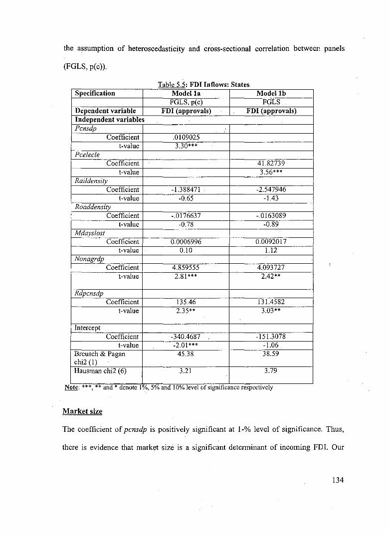
the assumption of heteroscedasticity and cross-sectional correlation between panels
(FGLS, p(c)).
Table 5 5· FDI Inflows· States .. Specification Modella Modellb
FGLS, p(c) FGLS Dependent variable FDI (approvals) FDI (approvals) Independent variables Pcnsdp
Coefficient .0109025 t-value 3.30***
Pcelecle Coefficient 41.82739
t-value 3.56*** Raildensity
Coefficient -1.388471 -2.547946 t-value -0.65 -1.43
Roaddensity Coefficient -.0176637 -.0163089
t-value -0.78 -0.89 Mdayslost
Coefficient 0.0006996 0.0092017 t-value 0.10 1.12
Nonagrdp Coefficient 4.859555 4.093727
t-value 2.81 *** 2.42**
Rdpcnsdp Coefficient 135.46 131.4582
t-value 2.35** 3.03**
Intercept Coefficient -340.4687 -151.3078
t-value -2.01 *** -1.06 Breusch & Pagan 45.38 38.59 chi2 (1) Hausman chi2 ( 6) 3.21 3.79
Note:***,** and* denote 1%,5% and 10% level ofs1gmficance respectively
Market size
The coefficient of pcnsdp is positively significant at 1-% level of significance. Thus,
there is evidence that market size is a significant determinant of incoming FDI. Our
134
findings clearly indicate that advantages of scale economies offered by larger domestic
markets positively influence FDI flows.
Infrastructure
The coefficient of the principal component of pcnsdp, pcelecon, and delcircle, viz.
pcelecle, is positively significant at 1-% level of significance. There are two
implications of this finding. Firstly, it reinforces the earlier finding regarding market
size. Secondly, it also indicates that availability of electricity and well-developed
communication networks are important determinants of FDI. It can be further concluded
that states with larger markets are likely to have greater presence of these infrastructural
facilities and are in more advantageous positions for attracting FDI.
Raildensity and rddensity are far from being significant. It appears that physical
infrastructure in terms of rail and road networks are not significant in determining
incoming FDI, as against electricity and telecommunications, which are strongly
significant. The insignificance of road and rail infrastructure probably imply that FDI in
India is geographically locating itself close to final product markets, thereby
overcoming the requirements of physical shipment of goods. The significant presence of .
FDI in non-tradeables can also partly explain the result. However, at the same time, it is
also clear that FDI is concentrating in activities requiring ready availability of electricity
and communication services, which are likely to be more IT -intensive sectors.
Degree of industrialisation
As per our hypothesis, the coefficients of nonagrdp appear with positive coefficients.
They are also statistically significant at 1% and 5% level of significance respectively.
·We therefore, conclude that more industrialised states are likely to attract greater FDI.
135
Quality of industrial relations
The coefficient of Mdayslost is not significant. This indicates that the quality of
industrial relations in states is perhaps not a deterrent for incoming FDI. It appears that
despite opinions expressed to the contrary (e.g. Lucas, 1993, Singh and Jun, 199.5),
incidence of strikes and lockouts, as reflected in workdays lost, has not acted as a
deterrent to FDI, at least in India.
Technological Capabilities and Infrastructure
The coefficients of rdpcnsdp are positively significant at 5% level of significance. The
results confirm our hypothesis. There is, thus, evidence of FDI flowing into states that
possess better technological infrastructure and indigenous technological capabilities.
Evidently, these locations offer greater opportunities for exploiting the ownership
advantages of FDI, much of which arise from possession of advanced technology and
know-how.
5.3.3 Macro-/eve/ analysis
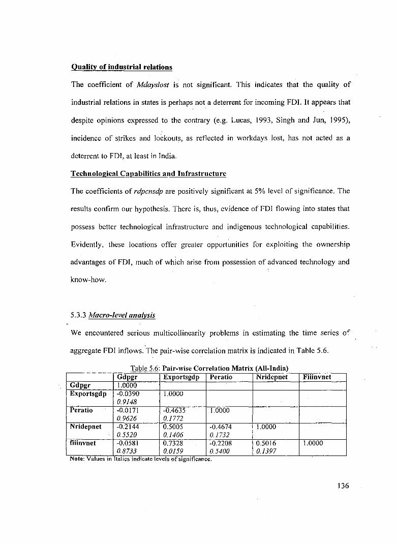
We encountered serious multicollinearity problems in estimating the time senes of
' aggregate FDI inflows. The pair-wise correlation matrix is indicated in Table 5.6.
Table 5 6· Pair-wise Correlation Matrix (All-India) Gdpgr Exportsgdp Peratio Nridepnet Fiiinvnet
Gdpgr 1.0000 Exportsgdp -0.0390 1.0000
0.9148 Peratio -0.0171 -0.4635 1.0000
0.9626 0.1772 Nridepnet -0.2144 0.5005 -0.4674 1.0000
0.5520 0.1406 0.1732 fiiinvnet -0.0581 0.7328 -0.2208 0.5016 1.0000
0.8733 0.0159 0.5400 0.1397 Note: Values m Italics md1cate levels ofs1gmficance.
136

In order to avoid multicollinearity, some variables were dropped, and the model was
estimated separately under different specifications. The estimations were carried out on
the basis of Ordinary Least Squares (OLS) technique. Robust estimation was used for
correcting heteroscedastic disturbances.
The results of our estimation are given in Table 5.7.
Table 5 7· FDI Inflows· All-India .. Modella Modellb Modellc OLS, robust OLS, robust OLS, robust
Dependent variable FDI (actual) FDI (actual) FDI (actual) Independent variable Gdpgr
Coefficient -525.9686 -795.5293 -796.9182 t-value -1.00 -1.11 -1.01
Peratio Coefficient -332.3093 -382.6154 -330.3041
t-value -2.86*** -3.60** -3.42**
Nridepnet Coefficient 0.4803497
t-value 1.30 Fiiinvnet
Coefficient 0.3969847 t-value 2.03*
Exportsgdp Coefficient 2686.51
t-value 1.81
Intercept 16236.89 20247.71 -1974.193 F-test F (3,6) =3.63*** F (3,6) =5.33** F (3.6) =7.07**
R-square 0.7568 0.7433 0.7695 RootMSE 3282.6 3320.7 3146.6 Note:***,** and* denote 1%,5% and 10% level ofs1gmficance respectively
137
Market size
We find that the coefficient of gdpgr is statistically insignificant. The result does not
confirm our hypothesis that FDI in India responds positively to growth in domestic
market size and also contradicts the findings of several empirical studies. The short
length of the time series can probably explain the result. Variations in real GDP growth
during this period (1992-93 - 2001-02) have been in the range of only around 3 .. 5
percentage points. Estimation of GDP growth over a longer time series might produce
different results.
Returns to capital
Stock market returns
The coefficient of peratio is found to be negatively significant. The result confirms our
hypothesis and indicates that FDI flows respond positively to lower values of peratio,
which arise when earnings from stock rrtarkets increase relative to prices. There is
therefore clear evidence ofFDI inflows being sensitive to returns from stock markets.
FII inflows
The coefficient of jiiinvnet is positively significant confirming our hypothesis. Thus,
there' is evidence that higher FII inflows, which occur from favourable expectations of
returns from the host economy, appear to encourage FDI also, through a 'demonstration
effect'. Since FII inflows are· strongly related to returns from stock markets, the latter
appear to be a major factor behind not only higher FII inflows, but also FDI flows.
Non-resident deposits
The coefficient of nridepnet is statistically insignificant. Thus, higher inflows of NRI
deposits are not a significant determinant for FDI
138
Export-orientation
The coefficient of exportGDP is also insignificant, The result corroborates the earlier
findings from the panel regression analysis, which suggest that export-intensity is not a
significant determinant ofFDI in India. FDI in India, therefore, is not export--oriented.
5.4 A SYNTHESIS
In this section, we try to present a synthesis of the results that we have obtained from
our industry-level, state-level and country-level analyses.
Industry-level analysis
Industry size is clearly a significant determinant of FDI in India. Industries with larger
sizes are seen to attract more FDI.
Although we expected FDI to flow into more capital-intensive industries, the positive
and significant coefficient of labour-intensity perhaps reflects the propensity of foreign
firms to invest in skill-intensive activities. These industries offer foreign firms ample
scope for exploiting their ownership advantages.
Import-intensity also emerges as a significant determinant of incoming FDI. Like skill
intensive industries, industries using more imported inputs in production offer foreign
firms considerable opportunities for better exploiting their ownership advantages again.
On account of better access to foreign inputs like imported raw materials, stores, capital
goods, know-how etc. multinationals are expected to be much more competitive than
domestic firms in import-intensive industrie~ and hence these are the sectors which may
attract larger FDI.
139

We had expected FDI to flow into more profitable industries. The results vindicate our
expectation. Profitability has a positive and significant impact on the level of FDI.
Results appear to be somewhat inconclusive with respect to advertising-intensity. If at
all, our results show that FDI is likely to be attracted to relative advertisement-intensive
· industries in India.
We have, however, obtained fairly clear evidence of FDI in India not being export-
oriented. Our results in this regard appear to confirm earlier findings of empirical
research, which point to FDI in India being more of the 'domestic market-oriented'
variety. The direction of causality between FDI and exports in India remains an
important agenda for future research47.
State--level analysis
The 'domestic market-oriented' nature of FDI in India gathers stronger evidence from
the results obtainkd in our state-level analysis. Market size is found to be a highly
significant locational determinant for FDI flows. It is clear that the advantages of scale
economies offered by large markets are important factors influencing FDI decisions in
India.
We have obtained interesting results regarding the role of infrastructure in motivating
FDI. We find that availability of electricity and communication facilities are critical
factors in deciding FDiflows. Rail and road networks, however, are not significant: Our
findings indicate that FDI has a clear tendency to locate close to markets for final
products. This tendency strengthens the decision to enter large markets and reinforces
47 Though FDI has not been found to be attracted to export-oriented industries, there is empirical evidence indicating that FDI has led to diversification of exports from traditional to non-traditional sectors in India. See Banga (2003).
140
the significance of market size~ We further argue that FDI in India probably has a larger
concentration in non-tradeables, for which, the locations of producers and consumers
are usually the same, thereby reducing the importance of facilities required for physical
shipment of goods. The significance of electricity and communication facilities also
points to the entry of FDI into sectors where the availability of these inputs is vital, i.e.
high technology, knowledge-intensive activities.
We hypothesised that more industrialised states are likely to attract greater FDI. Our
results point to similar conclusions. Degree of industrialisation of states is found to be a
significant determinant of FDI flows.
We did not find FDI flows to be sensitive to the quality of industrial relations.
The role of technological capabilities and infrastructure in attracting FDI is indeed ·a
significant result of our study., The positive significance of R&D expenditure at the
state-level to FDI flows clearly demonstrates the importance of possessing quality
teclmological infrastructure and technological capabilities at the local level for
attracting FDI. Our earlier results from the industry-level analysis, which point to the
inclination of FDI to move into skill-intensive industries, also acquire significance in
this regard. Availability of indigenous technological capabilities certainly enables
foreign firms to better utilise their ownership advantages.
Macro-level analysis
Our study of determinants of aggregate FDI inflows does not indicate market size to be
a significant determinant ofFDI. We attribute this result to the limited span of the time
series. However, it is important to mention in this context that we had employed growth
in GDP as our measure of market size. This measure is an indicator of potential market
141

size, rather than current size. It is possible that the results might have been different had
we used measures for the current size.
With respect to returns to capital, our findings regarding response of FDI flows to stock
market returns are indeed interesting. We find FDI flows to be positively related to
stock market returns. The results indicate that among other things, the returns earned on
equity capital deployed are important factors behind FDI decisions. We also find FII
inflows to positively encourage FDI through a 'demonstration effect'. This finding
corroborates our results on stock market returns. Indeed, buoyant domestic stock
markets and higher FII inflows are likely to encourage greater FDI flows into India. We
do not find inflows of non-resident deposits to be a significant determinant ofFDI.
We also find that FDI in India does not respond to exports. This reinforces our earlier
results that market size acts as a strong 'pull' factor for FDI in India. Our results appear
to confirm that FDI in India is essentially 'domestic market-oriented'.
142
A Note on the Data
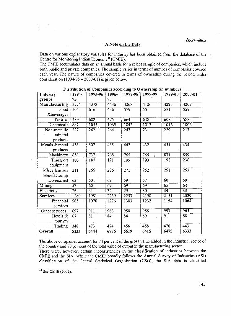
Data on various explanatory variables for industry has been obtained from the database of the Centre for Monitoring Indian Econom/8 (CMIE). The CMIE accumulates data on an annual basis for a select sample of companies, which include both public and private companies. The sample varies in terms of number of companies covered each year. The nature of co~panies covered in terms of ownership during the period under consideration (1994-95- 2000-01) is given below:
Distribution of Companies according to Ownership (in numbers) Industry 1994- 1995-96 1996- 1997-98 1998-99 1999-00 2000-01 groups 95 97 Manufacturing 3774 4372 4436 4268 4126 4225 4207
Food 505 616 636 579 551 581 559 &beverages
Textiles 589 682 675 664 638 608 588 Chemicals 887 1055 1069 1042 1017 1016 1002
Non-metallic 227 262 264 247 231 229 217 mineral
products Metals & metal 456 507 485 442 432 451 434
products Machinery 656 737 768 765 755 ' 831 859 Transport 180 187 191 199 193 198 236
equipment Miscellaneous 211 266 286 271 252 251 253 manufacturing
Diversified 63 60. 62 59 57 60 59 Mining 53 60 69 69 69 65 64 Electricity 26 31 32 29 30 34 33 Services 1280 1981 2239 2253 2190 2151 2029
Financial 583 ' 1070 1276 1303 1232 1154 1064 services
Other services 697 911 963 950 958 997 965 Hotels & 67 81 84 84 89 91 88
tourism Trading 348 473 474 456 458 470 443
Overall 5133 6444 6776 6619 6415 6475 6333
The above companies account for 74 per cent of the gross value added in the industrial sector of the country and 78 per cent of the total value of output in the manufacturing sector. There were, however, certain inconsistencies in the classification of industries between the CMIE and the SIA. While the CMIE broadly follows the Annual Survey of Industries (ASI) classification of the Central Statistical Organisation (CSO), the SIA data is classified
48 See CMIE (2002).
143

differently. In order to make the two sets of data compatible, the following matching exercise has been carried out:
Industries: SIA Industries: CMIE Modified format (1) (2) (3)
Metallurgical (ferrous, non- Ferrous metals, non-ferrous The four industries m (2) ferrous, special alloys, metals, mmmg, metals & have been grouped together mining & miscellaneous) metal products under metallurgy. Fuels (power, oil refinery, Petroleum products and The two industries in (2) have fuels) electricity been grouped together under
fuels. Electrical equipment Electrical equipment and The two industries in (2) have (electrical equipment, electronics (including been grouped together under computer software, computer computer) electrical equipment. hardware, electronics) Transportation industry Automobiles (including The two industries in (2) have (air/sea transport, passenger cars) and auto been grouped together under automobiles, passenger cars, ancillaries transportation. auto ancillaries, ports) Industrial machinery, Non-electrical machinery FDI for industries in ( 1) has machine tools, agricultural been accumulated to machinery, earth-moving represent FDI Ill non-machinery, miscellaneous 1 electrical machinery mechanical and engineering, commercial office & household equipment Fertilisers Fertilisers No change Chemicals (other than Chemicals No change fertilisers) Drugs & phannaceuticals Drugs & pharmaceuticals No change Textiles Textiles No change Paper & pulp including paper Paper & paper products No change products Sugar Sugar No change Fennentation industries Beverages & tobacco The industry in (2) has been
represented under fermentation industries
Food processing (food Food products Food products in (2) has been products & marine products) represented under food
processing Vegetable oils & vanaspati Vegetable oils & products No change Rubber goods Rubber and rubber products No change Soaps, cosmetics & .toiletries Soaps and detergents Industry Ill (2) has been
represented as soaps & detergents
Leather, leather goods & Leather products Industry m (2) has been pickers represented as leather. Cement & gypsum Cement Industry in (2) has been
represented as cement Services Services No change Hotel & tourism Hotel & tourism No change Trading Trading No change
144

Some industries from SIA had to. be excluded, as they could not be matched with the CMIE industries. These are: boilers & steam generating plants, prime movers other than electrical, telecommunication, medical and surgical appliances, industrial instruments, scientific instruments, photographic raw film and paper, dye stuffs, glue & gelatine, glass, ceramics and consultancy.
145
Appendix2 A Note on Principal Component Regression Method
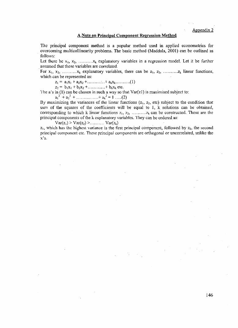
The principal component method is a popular method used in applied econometrics for overcoming multicollinearity problems. The basic method (Maddala, 2001) can be outlined as follows: Let there be x 1, x2, .......... xk explanatory variables in a regression model. Let it be further assumed that these variables are correlated. For x~, x2, .......... xk explanatory variables, there can be z1, z2, .......... zk linear functions, which can be represented as:
z, = a,x, + azXz + ............ + akxk .......... (1) Zz = b,x, + bzXz + ............ + bkxk etc.
The a's in (1) can be chosen in such a way so that Var(zl) is maximised subject to: 2 2 2 1 (2) a, +a2 + ............... +ak = .... .
By maximizing the variances of the linear functions (z1, z2, etc) subject to the condition that sum of the squares of the coefficients will be equal to 1, k solutions can be obtained, corresponding to which k linear functions z 1, z2, .......... zk can be constructed. These are the principal components of the k explanatory variables. They can be ordered as:
Var(z1) > Var(z2) > .......... Var(zk) z1, which has the highest variance is the first principal component, followed by z2, the second principal component etc. These principal components are orthogonal or uncorrelated, unlike the x's.
146