Chapter 5 Degradation of organic material

To appear in “Processes in Microbial Ecology”

To be published by Oxford University Press David L. Kirchman Draft: Feb 24, 2010

Chapter 5

Degradation of organic material

The previous chapter discussed the synthesis of organic material by autotrophic microbes,

the primary producers. This chapter will discuss the degradation of that organic material by

heterotrophic microbes. These two processes are large parts of the natural carbon cycle. Nearly

all of the 120 gigatons of carbon dioxide fixed each year into organic material by primary

producers is returned back to the atmosphere by heterotrophic microbes, macroscopic animals

and even autotrophic organisms (Chapter 4). Note the “nearly” in the last sentence. While

primary production is mostly balanced by degradation, imbalances occur, affecting many aspects

of the ecosystem. It is these imbalances that set whether the biota is a net producer or consumer

of atmospheric carbon dioxide. Since these imbalances depend on degradation as well as

primary production, so too do both primary production and organic matter degradation determine

the net contribution of the biota to fluxes of carbon dioxide to and from the atmosphere.

As with all biogeochemical cycles, the carbon cycle consists of reservoirs (concentrations

or amounts of material) connected by fluxes (time-dependent rates) made of both natural and

anthropogenic processes (Fig. 1). The natural rates of exchange between carbon reservoirs are

much larger than the anthropogenetic ones. In particular, the natural production of carbon

dioxide by heterotrophs is much higher than the anthropogenic production due to the burning of

fossil fuels and other human activities. The problem is that, because the anthropogenetic

production of carbon dioxide is not balanced by carbon dioxide consumption, concentrations in

the atmosphere are increasing and our planet is warming up (Chapter 1). Many of the natural

Chapter 5 OM degradation

2

processes in the carbon cycle are huge and variable. This complicates the efforts of

biogeochemists to understand how human activity is affecting the carbon cycle and to determine

the implications for climate change. One example is the missing carbon problem. Of the eight

petagrams of carbon burned by human activity every year, “only” about three stay in the

atmosphere. Some of the remaining five petagrams goes into the ocean or is taken up by plants

on land, but about three petagrams per year were missing until recently (Stephens et al. 2007).

While the missing carbon problem may be solved, many parts of the carbon cycle remain

mysteries, greatly complicating predictions of how the biosphere will respond to climate change

over the coming decades.

Figure 1 Global carbon cycle. The units for the numbers next to the reservoir names are Pg of carbon (Pg = 1015 g) and next to the arrows are PgC y-1. The numbers in parentheses are the yearly changes. Some features not shown here include the CO2 produced by land use change (2 PgC y-1) and the biggest carbon reservoir, carbonate rocks (Chapter 13). Some budgets use higher fluxes into and out of the oceans, closer to the rates seen for terrestrial systems (Sarmiento and Gruber 2006). Based on data presented in (Houghton 2007).


3

The carbon cycle has several reservoirs of both inorganic and organic material (Fig. 1).

The largest reservoirs are dissolved inorganic carbon (DIC), mostly bicarbonate, in the ocean,

and calcium carbonate (a major mineral in limestone) on land and in oceanic sediments.

Compared to the dissolved pools, the amount of carbon in organisms and in

non-living particulate organic is small. Aquatic ecologists call this dead material detritus, while

terrestrial ecologists also use the terms plant litter or simply litter when discussing material that

is still recognizable as coming from plants. Another large dissolved pool is dissolved organic

carbon (DOC), and there is also much organic carbon in sediments of the oceans. The largest

reservoir of organic carbon, however, is in soils and in other terrestrial compartments. These

organic reservoirs are as large (oceanic DOC) or larger (soil organic material) than the

atmospheric reservoir of CO2 which was 391 parts per million in January 2011, or over 760

gigatons for the entire atmosphere. Microbes are very important in setting the fluxes between

these large carbon reservoirs.

In this chapter, we discuss aerobic respiration and degradation of particulate detritus,

litter, and dissolved organic material (DOM) in oxic environments, leaving anaerobic respiration

in anoxic environments to later chapters. A simple equation for aerobic respiration is:

CH2O + O2 -> CO2 + H2O (1)

where CH2O symbolizes generic organic material, not a specific compound. In oxic

environments, the complete degradation of organic matter is due to aerobic respiration which

consumes oxygen and produces carbon dioxide and water. But degradation involves more than

just carbon because organic material nearly always has several other elements. Consequently,

organic matter degradation releases several other inorganic or mineral nutrients, such as

ammonium and phosphate, in addition to CO2 (Fig. 2). Some authors use “remineralization” to


4

highlight the never ending cycle of uptake and release of compounds containing essential

elements like N and P. The degradation and mineralization of detritus is the traditional role

assigned to heterotrophic microbes.

Figure 2. Mineralization of organic material by heterotrophic bacteria and fungi. LMW and HMW refer to low and high molecular weight material, respectively. Catabolism is the energy-producing parts of microbial metabolism whereas anabolic reactions lead to synthesis of cellular components and eventually growth. Some inorganic (“mineral”) compounds are potentially used by heterotrophic microbes (NH4

+, PO43- and Fe) whereas others (CO2, Ca2+

and Si) are not used substantially for energy production or biomass synthesis.

Mineralization of organic material in various ecosystems

Before discussing mineralization at the microbial scale, let us take a global view and

examine where mineralization and respiration are the highest. In the previous chapter, we saw

that roughly half of primary production was by land plants and the other half by microbes in the


5

ocean. As a first approximation, respiration is also split evenly between land and the sea. As

with primary production, respiration rates for the oceans, especially the open oceans, are rather

low when expressed per unit volume (m-3) or per unit area (m-2), but they add up to a large

number for the entire ecosystem because the oceans cover so much area and are so deep.

Likewise, respiration rates for lakes and rivers are low when averaged over the entire ecosystem,

but the per unit volume rates are actually quite high. Finally, in spite of covering only about

30% of the earth, soils account for nearly as much respiration as the oceans because of very high

per area rates.

As a general rule, degradation rates follow primary production, and the same ecosystems

with high primary production also have high rates of respiration (Fig. 3). Overall, there is an

excellent correlation between the two processes and the regression analysis indicates that

respiration and net primary production are in balance overall. However, there are important

exceptions when the two rate processes are not in balance. When primary production exceeds

respiration, the system is said to be net autotrophic, one example being spring blooms in aquatic

habitats (Chapter 4). Subsurface environments are net heterotrophic because primary production

is zero where light cannot reach. More intriguing to microbial ecologists and biogeochemists

are net heterotrophic aquatic systems in which respiration exceeds primary production. These

systems cannot long persist without the input of carbon from outside sources (allochthonous

carbon). A good example is a lake receiving large amounts of terrestrial organic material. These

lakes are often supersaturated with carbon dioxide and have much higher levels


6

of bacterial respiration and biomass production than expected from the in situ rates of primary

production. Like lakes, the oceans also receive organic material from land via rivers and rainfall.

Consequently, the oceans can be said to be slightly heterotrophic, although this input of

allochthonous organic carbon to the oceans on a global scale is so small that its contribution to

net heterotrophy would be difficult to measure directly. More controversial is whether large

regions of the oceans can be substantially heterotrophic for long (Robinson 2008), as mentioned

in Chapter 4. It is not clear why respiration is higher than net primary production for nine of the

twelve biomes in Figure 3. The difference between the two processes may not be significant

Figure 3. Respiration rates (R) and net primary production (NPP) in the major biomes of the world.The line is the 1:1 line. The slope and intercept of the regression line are not significantly different from one and zero, respectively (R=0.868NPP +11.6; r2 = 0.68), indicating that respiration follows net primary production. D=desert; U=tundra, G=temperate grassland, B=boreal forest, W=Mediterranean woodland, A=agriculture, S=tropical savannahs, F=temperate forest, T=moist tropical forest, O=open ocean, C=continental shelf, L=lakes. Data from(HPace and Prairie 2005H(HRaich and Schlesinger 1992H), (HBond-Lamberty and Thomson 2010H) and (HField et al

), .

Net Primary Production (mol C m-2 y-1)

0 20 40 60 80 100

Res

pira

tion

(mol

C m

-2 y-1

)

0

20

40

60

80

100

120

D

U

GB

W

AS F

T

O

C

L


7

considering the huge spatial and temporal variation in these numbers.

Who does most of the respiration on the planet?

In Chapter 4, we saw that microbes were responsible for about half of global primary

production due to photosynthesis by eukaryotic phytoplankton and cyanobacteria in the oceans.

Microbes account for much more than half of global respiration, although the precise percentage

is difficult to estimate. The global estimate may be less important than the percentages for

individual ecosystems. These percentages indicate the importance of microbes in structuring the

flow of carbon and other elements in these ecosystems.

In aquatic environments, respiration by microbes can be estimated by incubations in

which large organisms are removed by filtration, leaving only microbes in the water. The

consumption of oxygen is then measured over time in the dark (to stop photosynthesis and

oxygen production), sometimes along with the consumption of DOM. Simultaneously,

respiration by all organisms is estimated from changes in oxygen in other, dark incubations with

unfiltered water. This experiment has shown that nearly all of the respiration is by organisms <

200 μm in size (Fig. 4), which would include zooplankton and phytoplankton. Of more interest,

nearly half of total respiration is by organisms passing through a filter with 0.8 μm pores. The

exact percentage varies with the environment, but usually it is very high, 50% or greater. Other

analyses show that these organisms are mostly bacteria. Several other methods and approaches

support the conclusion that over half of total respiration in aquatic ecosystems is by bacteria.


8

Primary Production

0

20

40

60

80

100Respiration

%

of T

otal

<200 <53 <20 <2<5 <0.8Size Fraction (microns)

Figure 4. The size distribution of respiration and photosynthesis, expressed as a percentage of rates in unfiltered samples. Data from (HWilliams 2000H ).

It is much harder to compare respiration by microbes versus macroorganisms in

sediments and by bacteria versus fungi in soils. For macroorganisms in sediments the only way

devised so far has been to combine data on abundance and on rates per organism determined in

laboratory experiments. These studies indicate that macroorganisms account for 5-30% of total

respiration in freshwater and coastal marine sediments (Canfield et al. 2005). For soils,

respiration has been measured before and after removing plant roots. These studies found that

roughly half of total respiration is by roots (called autotrophic respiration) and associated

microbes in the rhizosphere (Andrews et al. 1999; Raich and Mora 2005), and nearly all of the

rest is by other microbes. Little respiration in soils is by large organisms, such as nematodes,

earthworms, and insect larvae, as their biomass is a small fraction (<5%) of total biomass in soils

(Fierer et al. 2009). Large soil organisms have a much more important role in breaking up large

pieces of plant litter and detritus, in the process creating more surface area for microbes to grow


9

and to degrade detrital organic material.

In contrast to aquatic ecosystems, on land fungi contribute substantially to soil

respiration. Here we focus on fungi living on dead organic material (saprophytic fungi), and

leave discussion of root-associated fungi (mycorrhizal fungi) to Chapter 14. According to

experiment using antibiotics and other inhibitors, bacteria and fungi account for about 35 and

65% of microbial respiration in soils, respectively (Joergensen and Wichern 2008). These

percentages may be inaccurate due to inefficiencies in stopping activity with inhibitors, and the

contributions by fungi and bacteria certainly vary among soils, depending on environmental

factors such as water content and temperature. Fungi do better than bacteria in dry soils, and

may also contribute more to respiration than bacteria at low temperatures (Pietikåinen et al.

2005). More so than bacteria, fungi degrade dead plants still standing above soil or water.

Like their contribution to respiration, the biomass of fungi as a fraction of total biomass is

much higher in soils than in aquatic habitats (Table 1). The exact percentage varies with the soil

type, geographical location, and method for estimating microbial biomass. It is possible to

examine both bacteria and fungi by epifluorescence microscopy (Chapter 1), yielding direct

counts of individual bacterial cells and estimates of total length of fungal hyphae. Both are then

converted to common units of grams of cellular carbon per gram of soil or sediment or per

milliliter of water. Other methods for estimating bacterial and fungal biomass also rely on

conversion factors and are imperfect. Regardless, the data indicate that fungi make up on the

order of 50% of microbial biomass in soils (Joergensen and Wichern 2008), but they are hard to

detect at all in lakes and oceans. Some fungi are indigenous to aquatic systems, and they may be

abundant on large particles and fresh detritus (Findlay et al. 2002), but their overall biomass is

low compared to bacteria in aqueous environments.


10

________________________________________________________________

Table 1 Abundance and biomass of bacteria and fungi in various habitats. “ND” is not detectable. The values depend on the location and time of sampling, varying as much as 10-fold. Data taken from (Frey et al. 1999), (Busse et al. 2009) and (Whitman et al. 1998).

Habitat

Bacterial abundance (106 cells ml-1 or g-1)*

Fungal length (m g-1)

Bacteria as % of Total Microbial Biomass

Soil, agriculture 900 164 71 Soil, forest 300 330 35 Lakes 1 ND 100 Ocean 0.5 ND 100 Marine Sediments 460 ND 100

* Abundance in lakes and oceans is expressed as 106 cells ml-1 (here surface waters) whereas in soils and sediments the units are g-1.

__________________________________________________________________

Bacteria and saprophytic fungi appear to have the same ecological role in nature, but their

abundance and contribution to total degradation are quite different in aquatic habitats versus in

soils. Why? Bacteria win out in the water column of aquatic habitats because their small size

makes them superior competitors for dissolved compounds. This competitive edge is less

important in soils, unless they are water-logged. In terrestrial environments, the hyphae life

form taken on by many fungi allows them to cross dry gaps between moist micro-habitats and to

access organic material not available to water-bound bacteria. Some bacteria also grow as

filaments, but the resemblance to fungal hyphae is superficial. Unlike bacteria, the cytoplasm of

fungi moves within the rigid hyphae to take advantage of favorable growth conditions. A

microbial ecologist in the 19th century thought of fungi as tube-dwelling amoeba (Klein and

Paschke 2004). The hyphal body form goes a long way to explaining the success of fungi in

soils.


11

Slow and fast carbon cycling pathways The amount of respiration, biomass, and biomass

production (Chapter 6) by bacteria versus fungi has several important implications for

understanding soil ecosystems (Moore et al. 2005). One is that bacteria are thought to mediate a

fast carbon cycling pathway while fungi are responsible for a slow pathway, reflecting the types

of organic matter used by the two microbial groups (Rinnan and Baath 2009). In soils bacteria

use labile organic compounds, while fungi degrade refractory material, the most important being

ligno-cellulose, as discussed below. These differences in organic carbon use have effects on

growth rates; as discussed in Chapter 6 in more detail, bacteria appear to grow more quickly than

fungi in soils. As a result of these growth rates, bacteria are said to mediate a fast pathway for

carbon mineralization while fungi do the same for a slow pathway. As with all generalizations,

there are exceptions, such as fungi growing quickly on labile organic material and bacterial

growing slowly on refractory detritus in aquatic habitats. But the slow-fast pathway model is

still a useful simplification for thinking about the implications of microbial growth.

High mineralization and respiration rates by microbes, whether bacteria or fungi, have

many implications for the flow of carbon in ecosystems, and radically transform the view of a

world with just plants, herbivores and carnivores. High respiration usually means high

degradation of organic material (Equation 1). Unless the organic material fueling respiration is

old and was synthesized by primary producers in the distant past, respiration by microbes

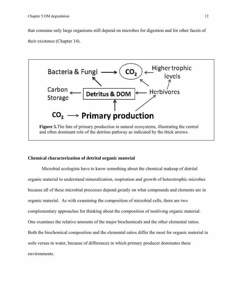
represents primary production not being used by herbivores whether on land or in water (Fig. 5).

So, when microbes account for most of total respiration, it implies that most of primary

production is routed through them and not through larger organisms. Given such high microbial

activity, it is sometimes amazing that large herbivores and carnivores exist on the planet. They

do exist because some take advantage of microbe-based food webs (Chapter 7). Even others


12

that consume only large organisms still depend on microbes for digestion and for other facets of

their existence (Chapter 14).

Figure 5.The fate of primary production in natural ecosystems, illustrating the central and often dominant role of the detritus pathway as indicated by the thick arrows.

Chemical characterization of detrital organic material

Microbial ecologists have to know something about the chemical makeup of detrital

organic material to understand mineralization, respiration and growth of heterotrophic microbes

because all of these microbial processes depend greatly on what compounds and elements are in

organic material. As with examining the composition of microbial cells, there are two

complementary approaches for thinking about the composition of nonliving organic material.

One examines the relative amounts of the major biochemicals and the other elemental ratios.

Both the biochemical composition and the elemental ratios differ the most for organic material in

soils versus in water, because of differences in which primary producer dominates these

environments.


13

While they share with phytoplankton many traits necessary for carrying out

photosynthesis, higher plants had to evolve several additional structures that are necessary for

success on land. Terrestrial plants need these structures in order to grow up and out into air

away from soil and to fend off attack by herbivores. Both problems are partially solved by plants

having lots of cellulose, related complex carbohydrates, and lignin, the latter being especially

abundant in wood. Cellulose is a polymer of glucose linked by β1,4 bonds whereas lignin is a

very complex, ill-defined structure consisting of several phenol groups (Fig. 6). Lignin is the

major component of wood and its strength explains why trees can grow so high. Lignin also

explains why wood is so hard for herbivores to eat. Although some phytoplankton and other

aquatic primary producers have cellulose in their cell walls, they do not make lignin. Suspended

by water, phytoplankton and macroalgae do not need lignin and woody structures to survive.

Figure 6. The structure of common subunits of lignin, the main structural element of wood. The amounts of these and other subunits vary with the type of lignin..

Consequently, phytoplankton are rich in protein, much more so than terrestrial plants,

because they lack many of the carbohydrates and all of the lignin required for life on land (Table

2). Some macroalgae have more carbohydrates, such as alginate, than phytoplankton, but still


14

not as much as terrestrial plants. Likewise, the particulate detritus in aquatic environments is

protein-rich whereas detritus on land reflects the carbohydrate make-up of terrestrial plants. The

chemical properties of carbohydrates and lignin that give terrestrial plants structural strength also

make them hard to degrade by microbes.

Other than the main biochemicals just listed, many components of detritus cannot be

assigned a chemical name. Unidentified components make up 50% or much more of detrital

mass, depending on the age of the detritus and stage of decomposition. The unidentified fraction

is low in fresh detritus and plant litter, but then increases with detritus age and as degradation

proceeds. Characterizing these unidentified organic compounds and determining how they are

formed are major topics in organic geochemistry.

Table 2. Biochemical composition of plant detritus and organisms in terrestrial and aquatic ecosystems. Data from (Canfield et al. 2005) and (Randlett et al. 1996). % of Total Lignin Carbohydrate Protein Lipid C:N Ratio Terrestrial Straw 14 81 1 2 80 Tree leaves 12 77 7 12 50 Pine wood 27 72 0 1 640 Aquatic Kelp 0 91 7 <1 50 Diatom 0 32 58 7 6.7 Zooplankton 0 14 46 <1 6.7

Biochemical composition drives the relative abundance of crucial elements making up

detritus and plant litter. Examining elements (usually C, N, and P) is the second approach for

studying DOM and particulate detritus. Aquatic organisms and detritus are rich in nitrogen

because of their high protein content whereas the opposite is true for terrestrial plants and

detritus. Another crucial element, phosphorus, is also more abundant in aquatic material relative


15

to its total mass. There is some nitrogen and phosphorus in plant detritus because, of course,

terrestrial plants have proteins, nucleic acids and lipids, but these N and P-rich compounds are

diluted by the high amounts of carbon in carbohydrates and lignin. Consequently, C:N and C:P

ratios are very high for terrestrial organic material, in contrast to the much lower ratios for

detritus in aquatic environments (Table 2).

Dissolved Organic Material As seen in Figure 1, the reservoir of DOC in the biosphere is

very large, much larger than that of particulate detritus, plant liter or of the biota. DOC is a large

component of DOM. In aquatic habitats, DOM is defined as whatever passes a filter with pore

sizes about 0.5 μm (Chapter 3). So, the DOM reservoir may have several things in it that are not

truly dissolved. As with particulate detritus, concentrations of DOM are usually expressed in

terms of key elements, mostly C, N and P. We know the most about DOC and less about

dissolved organic nitrogen (DON) and phosphorus (DOP). Soil ecologists focus on plant litter

and particulate detritus, but DOC and other DOM compounds are present in pore water of soils

and in aquifers. In soils the term “soluble organic material” is sometimes used instead of DOM.

Concentrations of DOC generally follow phytoplankton biomass levels (chlorophyll) and

primary production in aquatic habitats (Fig. 7). Surface waters of the open ocean have much

lower DOC concentrations than in euphotic reservoirs and lakes. Concentrations range from

about 50 μM-C in the winter of the Ross Sea (Antarctica) to over 500 μM-C in some eutrophic

lakes and reservoirs. Some of the DOC found in freshwaters comes from land, which explains

why concentrations are higher in freshwater than in marine habitats with similar phytoplankton

biomass levels. Terrestrial organic carbon makes its way to the oceans as well, but that input is

small compared to the marine DOC pool. Concentrations are usually higher in the euphotic


16

zones of both lakes and the oceans and then decrease with depth. In the deep ocean, DOC is

present at a minimum of about 35 μM-C. Most of the DOC in the biosphere is in the deep ocean

because its volume is so large.

Only about 10% of the DOM reservoir can be identified chemically. Some of the largest

components with known, defined structures include polysaccharides and proteins. The

concentrations of these two DOM components are usually estimated by measuring the monomers

resulting from acid hydrolysis of a DOM sample. The acid breaks up, for example, protein and

any amino acids complexed with other material, yielding “free” amino acids, which can be

measured by high performance liquid chromatography (described below). The difference then in

amino acid concentrations before and after acid hydrolysis gives an estimate of the dissolved

combined amino acid concentrations. The same procedure is used to estimate free and combined

carbohydrates. Great progress is being made in characterizing DOM using techniques such as

mass spectrometry- Fourier transform ion cyclotron resonance (FT-ICR-MS) (Dittmar and Paeng

2009).

Chlorophyll (μg liter-1)

0.1 1 10

DO

C (μ

M-C

)

50

75

250

500

750

100

LakesMarine

Figure 7. DOC in the surface layer of some lakes and oceans. Data are from (HDel Giorgio et al. 1999H) and (HKirchman et al.

2009H)


17

The concentrations of simple monomers like free amino acids and sugars are usually very

low, about 10-fold lower than combined forms. In aquatic habitats, the concentration of each

free amino acid may range from <1 to 20 nM and the total concentrations are usually <100 nM.

To put this concentration in perspective, there are more amino acids on your fingertips than there

are in a liter of water. Concentrations in soils are much higher, in the micromolar range (Jones et

al. 2009), perhaps because some of the measured monomers are released during the extraction of

soil pore waters. Even in soils, however, concentrations of simple monomers are much lower

than concentrations of the polymers they occur in. That is, concentrations of free glucose, other

sugars, and amino acids are much lower than concentrations of polysaccharides, peptides, and

proteins.

Much of soil organic material and DOM in aquatic habitats is said to be humic material.

This and related terms came from soil chemists examining fractions of soil organic material

isolated by acid and base extractions and other simple procedures. The fractions are defined by

the isolation procedure, resulting in material with predictable bulk characteristics (Fig. 8). The

structure of humic material is often depicted as being incredibly complicated with many aromatic

rings, studded with phenolic (-OH) and organic acid (-COOH) moieties (Stevenson 1994). The

ligno-cellulose detritus from terrestrial plants has humic-like properties and some classic humic

moieties. This detritus can be abundant in small lakes and rivers receiving large inputs of

terrestrial organic material. But the classic model of humic substances probably does not

accurately reflect the chemical composition of organic material in soils and aquatic habitats

(Kleber and Johnson 2010). It is difficult for any single model to capture the complexity of

natural organic material in soils and aquatic habitats.


18

Figure 8. Classic definitions of organic material fractions isolated from soils. The terms, especially humic acids, are often used to describe DOM in aquatic habitats. Based on (HStevenson 1994H).

Detrital food webs

Detritus and plant litter are produced when phytoplankton, higher plants, and animals

senesce and die. Detritus also can be a byproduct of herbivore grazing or of lysis by viruses.

One type of detritus is the fecal material from metazoan grazers, which varies in size depending

on the grazer and the prey concentration. Even protists can produce submicron particles

(“picopellets”), although many of these particles would be included in the DOM reservoir.

Dissolved compounds can also stick together--coagulate-- and form particulate detritus in aquatic

systems. The detritus produced by these different mechanisms differs in composition and rates

of degradation.


19

Detritus supports a complicated food web of bacteria, fungi, protists and metazoans, all

living directly or indirectly on particulate dead organic material rather than on live plants or

algae. Detrital food webs are especially important in detritus-rich habitats, such salt marshes,

many estuaries, bogs, and all soils. In addition to large reservoir sizes, the flux of detritus and

plant litter is also very high. Nearly all primary production from trees is routed through detrital

food webs while roughly half is in the case of grasslands (Cebrian 1999). The percentage may

be equally high in detritus-rich aquatic habitats, such as small ponds and salt marshes, but it is

low (<10%) in the open ocean and large lakes without high amounts of particulate detritus.

Many types of organisms are able to ingest detritus and potentially obtain some carbon,

other elements, and energy, if not use it as a sole food source (Table 3). These organisms are

called detritivores. Marine benthic ecologists use the term deposit-feeders, reflecting the fact

that detritus is deposited onto sediments from plankton production in overlying

surface waters. In the water column of aquatic habitats, relatively few metazoans seem to

specialize on detritus, as the grazers there are more selective and ingest individual food items,

although some filter-feeding zooplankton do appear to ingest all particles of the certain size. In

contrast, in sediments and soils where detritus, plant litter, and inorganic particles are much more

Table 3. Some examples of detritivores, which are eukaryotes able to consume detritus and use it for carbon, other elements, and energy. Bacteria and other microbes associated with the detritus may be as important as or more so than the detrital carbon itself to these organisms.

Habitat Organism Comments Aquatic water column Zooplankton Most are mainly herbivores and carnivores

Aquatic sediments Nematodes Aquatic sediments Harpacticoid copepods Aquatic sediments Polychaetes Mainly marine Soils Enchytraeids Microdrile annelids, commonly known as

“potworms” Soils Oligochaetes Megadrile annelids, including earthworms Soils Nematodes Soils Collembola Small arthropods (<5 mm)


20

abundant, detritivores feed more indiscriminately. Many of these organisms are classified by

size (Fig. 9).

Figure 9. Organisms are often grouped by size set by the nets and sieves used for collection. Only a few of many possible organisms are given here as examples. “Meiofauna” is used by sediment ecologists while soil ecologists prefer “mesofauna”. Many of these organisms are capable of feeding on detritus and detritus-associated microbes. See also Table 3 for more examples.

In all cases, microbes, which otherwise are too small to be grazed on by these animals,

are included with the detritus as it is ingested. Which is more important nutritionally to the

animal, the detritus or the attached microbes? With few exceptions, the detritus has more

organic carbon than the microbes in terms of sheer mass. However, microbes may be more

nutritious because of their high protein content, whereas detritus consists largely of structural

polysaccharides, such as ligno-cellulose, depending on its age and source. Even with the help of


21

symbiotic bacteria (Chapter 14), these polysaccacharides are difficult for metazoans to digest and

are low in nitrogen. So, there is no simple answer to the microbes versus detritus question. The

relative contribution of each to animal nutrition depends on the detritus and the detritivore.

A B

Figure 10. Effect of macrofauna-like worms on the degradation of organic material and on the structure of soils and sediments. Panel A illustrates a worm-less world in which large pieces of detritus are not broken down. In contrast, in the environment depicted by Panel B, worms and other macrofauna help to break up detritus and facilitate the mineralization of the organic material to inorganic nutrients like ammonium and phosphate. The burrows of these large organisms also allow faster diffusion of gases in soils and of dissolved compounds in aquatic sediments.

Detritivores are very important in effecting the degradation of particulate detritus in both

terrestrial and aquatic ecosystems, even though their direct contribution to detritus mineralization

is small. Rather than accounting for much respiration, the more important role of detritivores is

to physically break up detritus and plant litter, which decreases the size of detrital particles and

as a result increases the surface area where microbes can adhere and degrade the exposed organic

compounds (Fig. 10). Macrofauna (organisms larger than 2 mm) can have additional effects on

the microbial environment. In soils, these large animals (large in the microbial world) break up

aggregates and increase aeration and water flow. Earthworms in particular constitute a

“geomorphic force” orders of magnitude stronger than other, purely physical processes (Chapin


22

et al. 2002). Likewise, in sediments, burrows of macrofauna allow penetration of oxygen into

otherwise anoxic environments, greatly affecting sediment chemistry. In both soils and

sediments, macrofauna disrupt the orderly layers, horizons and gradients in geochemical

properties that would otherwise form in a world without animals. The end result is that

detritivores and other macroscopic organisms help to speed up the degradation of detritus even

though most of the actual mineralization is done by bacteria and fungi.

DOM and the microbial loop

In addition to particulate detritus, plant and algal organic material becomes available to

microbes when it is transferred from cells and particulate detritus to dissolved reservoirs. In

soils and sediments with rooted plants, this release is part of below-ground production, in

contrast to the more visible above-ground production. Although difficult to estimate, below-

ground production can be a very large fraction (as high as 50%) of total primary production by

higher plants (Högberg and Read 2006). Dissolved or soluble organic material released by roots

fuels soil microbial activity while bypassing herbivores.

Like excretion by plant roots, DOM is released directly by phytoplankton in aquatic

ecosystem, but it is also produced by many heterotrophic organisms. The release of DOC by

phytoplankton can be measured by tracing 14CO2 into phytoplankton cells and eventually into the

DOM reservoir. These experiments indicated that as much as 50 % of primary production can be

released as DOM, although the overall average is probably closer to 10%. Some of the 14C-

labeled DOC comes directly from phytoplankton cells, while other components may be released

inadvertently by herbivores trying to eat phytoplankton cells, a process sometimes called sloppy

grazing. Still other DOM is released during excretion by herbivores and carnivores in aquatic


23

ecosystems. The internal content of cells lysed by viruses also adds to the DOM reservoir

(Chapter 8). Since bacterial respiration amounts to about 50% of primary production but only

10% of it comes from direct phytoplankton excretion, most of the DOM production must be by

mechanisms involving organisms other than phytoplankton. This complicates efforts to compare

bacterial production and respiration with primary production (Chapter 6).

In addition to containing large amounts of carbon and other elements (large reservoir

size), fluxes through the DOM reservoir are also quite large and can support much microbial

growth and respiration. In soils, it is difficult to compare the relative importance of DOM with

that of particulate detritus in supporting microbial activity, but DOM accounts for at least 50%,

on average, of soil respiration because that is the percentage attributable to root exudation and

below-ground production. This is a high percentage even if we assume that the other 50% is

from particulate detritus. In aquatic habitats, it is easier to compare the activity of “free-living”

and particle-associated bacteria. 3H or 14C-labeled dissolved compounds, such as glucose or

amino acids, are added to a water sample and incubated for an hour or so. Then the radioactivity

in attached microbes is collected by filtration using large pore-sized filters (1 or 3 μm) and

compared to the radioactivity going through these filters.

This type of experiment demonstrates that usually >75% of total bacterial activity is by

free-living cells rather than the particle-associated ones. Any uptake by non-bacterial microbes,

such as fungi, large phytoplankton, and other protists, which are in the large size fraction, would

lead to even higher estimates for the free-living cells relative to the attached bacteria. The

percentage may be lower if some of the particles are broken up by the filtration process. Also,

the apparently free cells may in fact be associated with small particles that pass through GF/F

filters (Chapter 3) used to separate the dissolved and particulate pools.


24

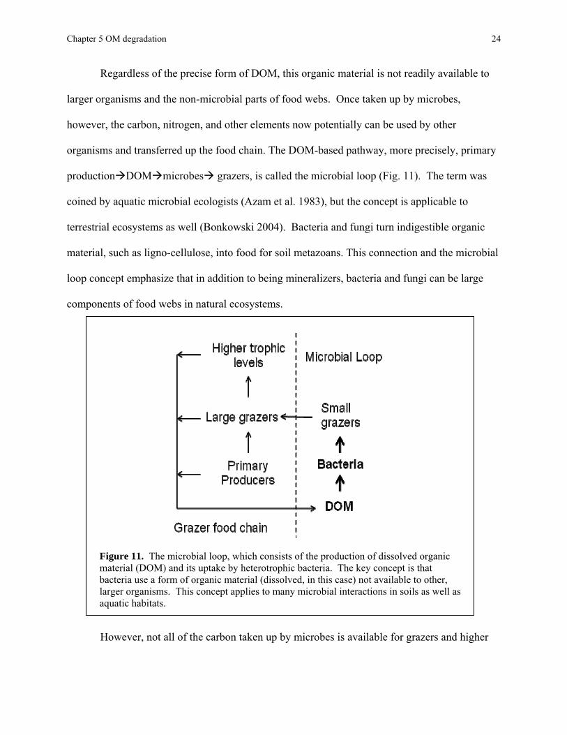
Regardless of the precise form of DOM, this organic material is not readily available to

larger organisms and the non-microbial parts of food webs. Once taken up by microbes,

however, the carbon, nitrogen, and other elements now potentially can be used by other

organisms and transferred up the food chain. The DOM-based pathway, more precisely, primary

production DOM microbes grazers, is called the microbial loop (Fig. 11). The term was

coined by aquatic microbial ecologists (Azam et al. 1983), but the concept is applicable to

terrestrial ecosystems as well (Bonkowski 2004). Bacteria and fungi turn indigestible organic

material, such as ligno-cellulose, into food for soil metazoans. This connection and the microbial

loop concept emphasize that in addition to being mineralizers, bacteria and fungi can be large

components of food webs in natural ecosystems.

Figure 11. The microbial loop, which consists of the production of dissolved organic material (DOM) and its uptake by heterotrophic bacteria. The key concept is that bacteria use a form of organic material (dissolved, in this case) not available to other, larger organisms. This concept applies to many microbial interactions in soils as well as aquatic habitats.

However, not all of the carbon taken up by microbes is available for grazers and higher


25

trophic levels. Some of it may be respired as CO2 and thus is lost from the system until it is

fixed again by primary production. The rest of the carbon taken up by microbes would be used

for biomass production and would be available as food for grazers. Figuring out which of these

two fates of carbon—respiration or biomass production—is most important has been called the

“sink or link” question (Pomeroy 1974). Is the microbial loop a sink in which the carbon is

mostly respired and lost from the system? Or is it a link, meaning that organic carbon taken up

by microbes is passed on to higher trophic levels? Which fate dominates?

For aquatic ecosystems, the sink-link question was answered experimentally by

examining the use of 14C-glucose by bacteria and the rest of the plankton. This radioactive form

of glucose was added to large mesocosms (big bags containing 10 to >1000 liters of water) and

the radioactivity was then followed in organisms with various sizes over several days.

Figure 12. The fate of 14C-glucose added to a mesocosm. Note the large amount of 14C radioactivity (given here as dpm) in the small size fraction (0.2 to 1.0 μm) and small amount in the larger size fractions, indicating that most of the organic carbon was assimilated by bacteria and then respired rather being transferred to larger organisms and higher trophic levels. This experiment indicated that the microbial loop is a sink. Data from (HDucklow et al. 1986H).

0

1

2

3

4

5

6

7

Time (d)

14C

radi

oact

ivity

(104 d

pm L

-1)

0.2 - 1.0 μm1-3 μm 10-35 μm

0 2 4 6 8 10 12 14


26

Microbial ecologists found that little of the radioactivity appeared in large organisms, implying

that little of the glucose taken up by bacteria was transferred to other food chains (Fig. 12). The

link between the microbial loop and larger organisms was weak. Most of the radioactivity was

simply respired to CO2, indicating that the microbial loop is mainly a sink.

This conclusion was later supported by data on the bacterial growth efficiency (BGE).

This parameter is the ratio of biomass production (P) to the sum of production and respiration

(R):

BGE = P/(P + R) * 100 (2).

When the sink-link question was first posed, microbial ecologists thought that the growth

efficiency of bacteria was high, on the order of 50%. Growth efficiencies of fungi were also

thought to be high. However, results from new experiments with natural microbial communities

indicated that the growth efficiency was much less than 50%, ranging from 15% in the oceans to

35% in estuaries (Fig. 13). Even less is known about growth efficiencies of microbes in soils,

aside from respiration of simple compounds like glucose and acetic acid (Six et al. 2006)(Herron

et al. 2009), which suggest perhaps higher efficiencies for soil microbes than for aquatic bacteria.

There is little reason to believe that fungi and bacteria differ in growth efficiency, if they use the

same organic material, since heterotrophic metabolic pathways are the same in both. In any case,

growth efficiencies less than 50% mean that most of the carbon is released as CO2 and little

remains in biomass available to be eaten and passed onto higher trophic levels. So, the low

growth efficiency estimates indicate that the microbial loop is mainly a sink.

Still, the microbial loop is also a link, transferring otherwise unavailable material and

energy, starting as DOM or complex detritus, to larger organisms and higher trophic levels. The

link percentage is similar to the percentage of C transferred by small other, traditional food webs.


27

This question has been examined by adding 14CO2 or 14C-glucose to separate incubations of lake

water and then tracing the 14C into large zooplankton (Wylie and Currie 1991). The labeled

glucose traces transfers by the microbial loop as discussed below while 14CO2 is used to follow

carbon fixed by primary producers and then transferred by a traditional grazer food chain. When

normalized to the initial 14C uptake, roughly equal amounts of 14C ended up in the large

zooplankton, suggesting transfer of bacterial carbon to large organisms was similar to the

transfer of phytoplankton carbon. The key is the number of trophic levels and transfer steps

before the top of the food chain is reached (Berglund et al. 2007). It does not matter whether

those steps are taken by bacteria and other microbial loop components or by metazoans. The

effect of the number of trophic levels on transfer up food chains is discussed again in Chapter 7.

0

10

20

30

40Ocean Rivers Lakes Estuaries

Organic carbon availability

Gro

wth

Effi

cien

cy

Figure 13. Growth efficiencies for natural ecosystems. One hypothesis to explain variation in growth efficiency is the amount and quality of organic carbon. Data from (Del Giorgio and Cole 1998).


28

Hydrolysis of high molecular weight organic compounds

Even after detritus and plant litter is broken up by metazoans, organic compounds may

need to be reduced in size even further before use by microbes. Organic compounds larger than

about 500 Da must be transformed somehow to smaller compounds which can then be

transported across cell membranes. This transformation usually consists of hydrolysis of

polymers to monomers; hydrolysis, which literally means “lysis by water”, is the breaking of

bonds that link monomers together into a polymer. For example, hydrolysis of protein releases

amino acids and oligopeptides, but not CO2 nor NH4+. Hydrolysis is often said to be the rate-

limiting step or the slowest reaction in the degradation pathway, one piece of evidence being that

concentrations of polymers are higher than that of monomers.

The 500 Da cutoff for transport is largely set by the capacity of transport proteins

embedded in cell membranes to ferry substrates from the environment across the membrane and

into the cell. The 500 Da limit applies to other organisms, not just bacteria. Although metazoans

and protists can capture and retain food in a digestive tract or food vacuole, they still must use

enzymes to hydrolyze high molecular weight (HMW) compounds, which make up the bulk of

their food, before the organic material can be used. In metazoans and protists, these enzymes are

excreted into digestive tracts and food vacuoles where they work on HMW compounds. The

released compounds <500 Da are then transported into the protist cell or into cells lining the

metazoan digestive tract.

Several types of enzymes, collectively called hydrolases, are needed to hydrolyze

polymers found in HMW pool (Table 4). Specific enzymes are necessary for each biopolymer,

with the enzyme name usually containing the polymer name, such as cellulases for cellulose and

proteases for protein. For most polymers, effective hydrolysis requires enzymes that work on


29

different parts of the polymer chain. The breakdown of protein is a good example (Fig. 14).

Protein must first be hydrolyzed by exoproteases, which cleave off amino acids or dipeptides

(two amino acids) at the ends of the polypeptide, and endoproteases, which cleave the peptide

chain far from the ends. Exoproteases can be further divided into those that work at the N

terminus (aminopeptidases) or at the C terminus (carboxypeptidases) of the peptide chain. Any

oligopeptides must then be hydrolyzed further by peptidases, although this hydrolysis step may

be inside the cell if the oligomer is <500 Da, or roughly a pentapeptide. Finally, the monomers

can be used to synthesize new polymers or they are catabolized to provide energy. Note that

only during catabolism of monomers, the final step in biopolymer degradation, is organic carbon

oxidized to CO2 and nitrogen mineralized to NH4+.

Table 4. Some polymers, associated hydrolase, and fluorogenic analogues used to study hydrolyase activity.

Biopolymer Hydrolyase Analog*

Proteins leucine aminopeptidase, Leu-MCA Chitin, glycoproteins N-acetyl-β-D-

glucosaminidase MUF-N-acetylglucosamine

Peptidoglycan

Lysozyme MUF-N- tri-N-acetyl-β-chitotrioside

Chitin Chitinase MUF-N- tri-N-acetyl-β-chitotrioside

Organic phosphate Phosphatase MUF-phosphate Cellulose Cellulase MUF-β-D-cellobioside Polysaccharides with alpha-linkage

α-D-glucosidase MUF- α-D-glucoside

Lipids Lipases Various *MCA= methylcoumaryl; MUF= methylumbelliferyl

Enzymes that catalyze the initial hydrolysis of biopolymers into low molecular weight

(LMW) byproducts must be located outside of the outer cell membrane, hence their name


30

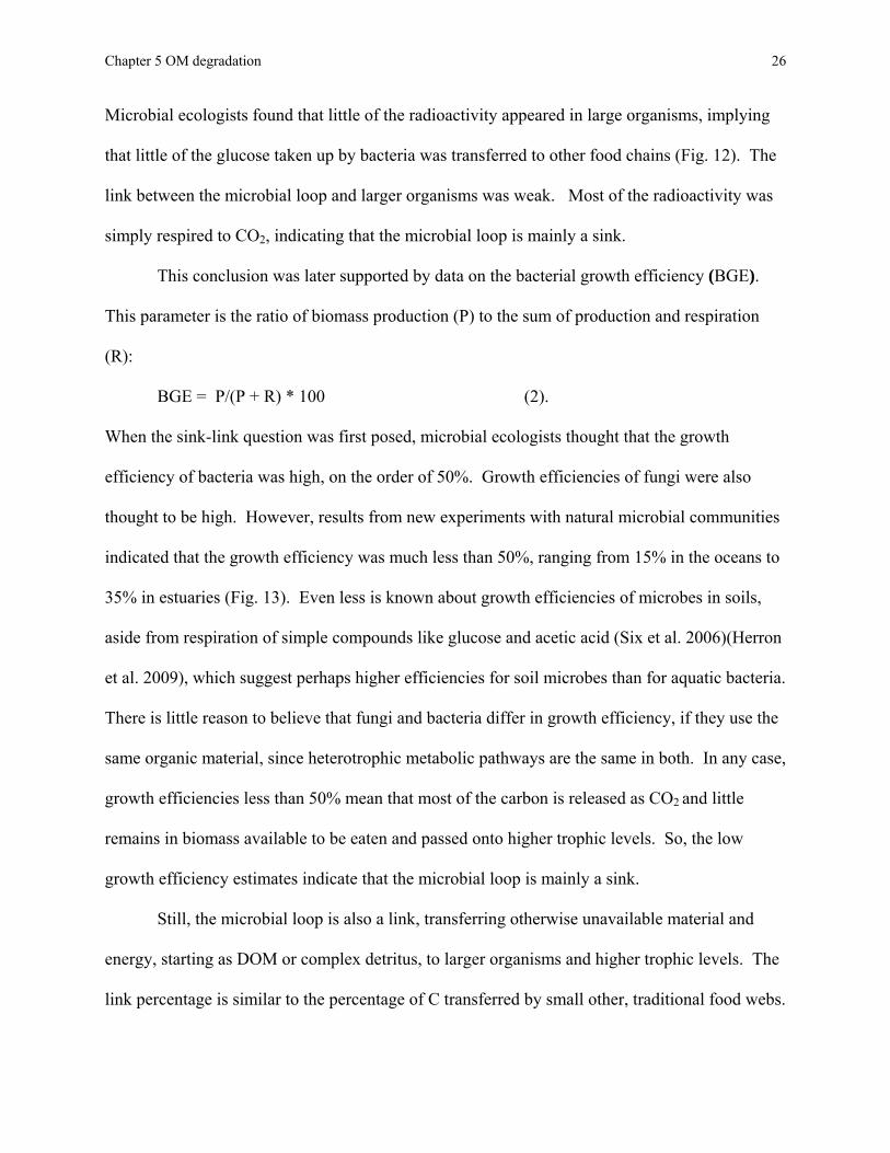
extracellular enzymes. Another term is ectoenzymes. Analogous to the food vacuole of protists

and the digestive system of metazoans, releasing extracellular enzymes to the outer environment

is an effective strategy for bacteria in biofilms or in particulate detritus. Likewise for microbes

in a soil aggregate. In these cases, the released enzyme has a good chance of reaching the

targeted biopolymer (concentrations are high) and in turn, the LMW byproducts cannot diffuse

away before uptake by the cell originally releasing the enzyme.

+NH3

COO-

aminopeptidase endopeptidase carboxypeptidase

. . . .

+NH3 COO-

AA AA1-AA2-AA3-AA4AA1-AA2

peptidases

AA1-AA2 AA1-AA2-AA3-AA4

catabolism or protein synthesis

AA

Figure 14. Example of the enzymes needed to degrade high molecular weight organic material. AA is a free amino acid.

Most free-living bacteria, especially in aquatic environments, must use a different

mechanism. In these environments, any LMW byproducts resulting from biopolymer hydrolysis

would diffuse away from the cell synthesizing and releasing the hydrolase. Other cells may

“cheat” and utilize the LMW byproducts without incurring the cost of enzyme synthesis. The

released enzyme itself would be a good carbon and nitrogen source for other microbes. Rather


31

than releasing enzymes, free-living bacteria in natural environments seem to have these enzymes

somehow attached or tethered to the outer membrane. Nearly all biopolymer-hydrolyzing

enzymes are cell-associated and little enzyme activity is found in the dissolved reservoir in

aquatic environments. There are times, however, when activity of some enzymes in the

dissolved phase is high for unknown reasons.

Lignin degradation One of the most abundant types of HMW organic material is lignin.

Although composed of characteristic compounds (Fig. 8), lignin is not a polymer with regular,

repeating bonds like a protein or carbohydrate. Consequently, it is broken down by a mechanism

quite different from how other biopolymers are degraded. One key to lignin degradation is the

production of hydrogen peroxide (H2O2) by a variety of mechanisms, such as the excretion of

aldehydes which are oxidized by extracellular enzymes to hydrogen peroxide. This highly

reactive compound then serves as a co-substrate for several enzymes, such as lignin peroxidase,

manganese-dependent peroxidase, and copper-dependent laccase, to attack lignin. The exact

details of lignin degradation remain unclear.

In soils, white rot fungi are the main degraders of lignin, with Phanerochaete

chrysosporium, belonging to the homobasidiomycetes being the best studied example (Cullen

and Kersten 2004). The name includes “white” because degradation of the brown, lignin-rich

parts has the net effect of bleaching the wood. In contrast, brown rot fungi focus mainly on the

white parts rich in cellulose and hemicelluloses, leaving behind the darker, lignin-rich

components. Studies using both radioactive 14C and stable 13C indicate that lignin carbon is not

used for biosynthesis by fungi, nor is it likely broken down to generate energy, given that lignin


32

degradation occurs extracellularly. Rather, white rot fungi appear to degrade lignin to gain

access to more easily degraded cellulose and hemicelluloses in wood detritus.

Bacteria are not important in degrading lignin in soils, and no bacterium has been isolated

so far that completely degrades wood (Zimmermann 1990). Fungi are probably superior

degraders of wood and lignin specifically because of their enzymes and hyphal growth form.

However, bacteria may be more important than fungi in aquatic environments where their sheer

numbers give them an advantage. This question has been examined by following the fate of the

recalcitrant (lignin) or the more labile part (cellulose) of lignocellulose complexes labeled with

14C in incubations with added inhibitors that act against either bacteria or fungi (Benner et al.

1986). Bacteria account for what little lignin degradation occurs in anoxic environments where

fungi and most other eukaryotes cannot survive.

Uptake of low molecular weight organic compounds: turnover versus reservoir size

After hydrolysis or the breakdown of large compounds, the next step in organic material

degradation is the assimilation of monomers and other LMW compounds. These compounds

could come from microbial hydrolysis of biopolymers, but monomers and other LMW

compounds can also be released by plant roots in soils and by phytoplankton and zooplankton in

aquatic environments. We know the most about the fate of free amino acids and glucose. These

compounds have been examined extensively because proteins and polysaccharides are large

components of cells and of the known fraction of organic material. In addition, the use of amino

acids and some sugars can be followed easily because their concentrations can be measured by

high pressure liquid chromatography (Fig. 15) and they are available labeled with 13C, 14C, or 3H


33

Fig. 15. Quantifying compounds in complex mixtures by high performance liquid chromatography (HPLC). Microbial ecologists use HPLC to estimate concentrations of one or more compounds in mixtures of several compounds. As with all types of chromatography, the basic principle is that compounds differ in their affinity for the solid material in the column versus the solvent or mobile phase carrying the compounds. This difference in affinity results in differences in the time (elution time) that the compound is retained in the column. Because the small bead size results in high pressure, sometimes the “p” in HPLC means “pressure”.

If judged by concentrations alone, LMW compounds would not seem very important in

fueling microbial growth and in overall degradation of organic material. However, in spite of low

concentrations, the flux of amino acids and other monomers can be quite high. Flux refers to

both production and uptake, which are equal at steady state (dS/dt =0). The change in a

compound (or substrate, S) over time is:

dS/dt = P - λS (3)


34

where P is the production rate and λ the turnover rate constant. The units of flux combine the

units of both concentration (mass per unit area or volume, such as nanomol liter-1) and of the

turnover rate constant (per time, such as per day). In spite of very low concentrations, turnover

is fast enough to result in very high fluxes (Fig. 16). Microbial ecologists often use the inverse

of turnover rate constants, the turnover time, to quantify the relationship between fluxes and

reservoir size. Geochemists use “residence time” for the same concept.

Figure 16. Relationship between reservoir size and fluxes. Not shown are cases in which a low flux is due to a small reservoir and a high flux due to a large reservoir.

The turnover time of LMW compounds like amino acids can range from minutes to

hours, even at the high concentrations found in soils (Jones et al. 2009). The end result is that

the flux of free amino acids or of glucose alone can support a high fraction, sometimes all of

bacterial growth in natural environments (Kirchman 2003). More generally, low concentrations

of a compound may result from low production, but they may also result from high production


35

and rapid use by microbes.

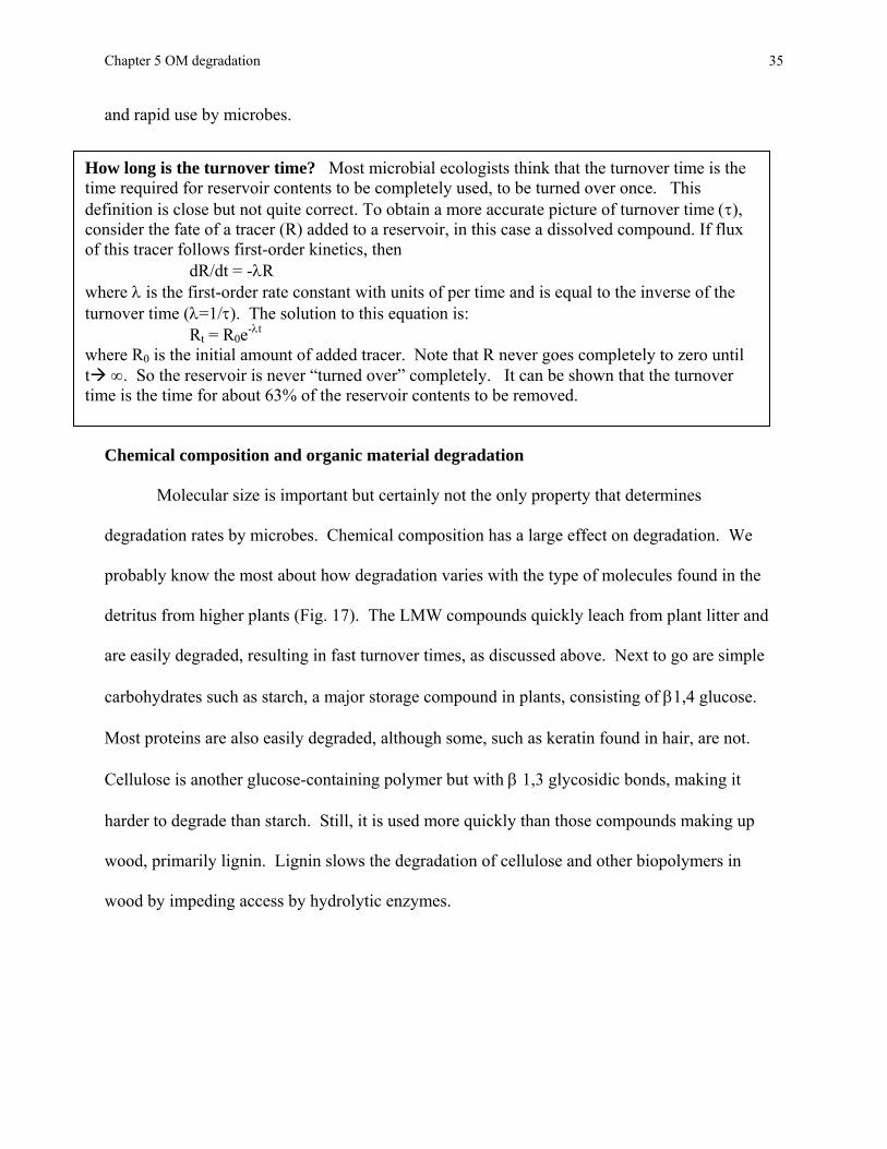
How long is the turnover time? Most microbial ecologists think that the turnover time is the time required for reservoir contents to be completely used, to be turned over once. This definition is close but not quite correct. To obtain a more accurate picture of turnover time (τ), consider the fate of a tracer (R) added to a reservoir, in this case a dissolved compound. If flux of this tracer follows first-order kinetics, then dR/dt = -λR where λ is the first-order rate constant with units of per time and is equal to the inverse of the turnover time (λ=1/τ). The solution to this equation is: Rt = R0e-λt where R0 is the initial amount of added tracer. Note that R never goes completely to zero until t ∞. So the reservoir is never “turned over” completely. It can be shown that the turnover time is the time for about 63% of the reservoir contents to be removed.

Chemical composition and organic material degradation

Molecular size is important but certainly not the only property that determines

degradation rates by microbes. Chemical composition has a large effect on degradation. We

probably know the most about how degradation varies with the type of molecules found in the

detritus from higher plants (Fig. 17). The LMW compounds quickly leach from plant litter and

are easily degraded, resulting in fast turnover times, as discussed above. Next to go are simple

carbohydrates such as starch, a major storage compound in plants, consisting of β1,4 glucose.

Most proteins are also easily degraded, although some, such as keratin found in hair, are not.

Cellulose is another glucose-containing polymer but with β 1,3 glycosidic bonds, making it

harder to degrade than starch. Still, it is used more quickly than those compounds making up

wood, primarily lignin. Lignin slows the degradation of cellulose and other biopolymers in

wood by impeding access by hydrolytic enzymes.


36

We can draw some generalizations from studies of the plant litter degradation and of

organic pollutants about how chemical structure affects degradation rates. In general, the bonds

of large, naturally-occurring polymers with many branches are difficult for microbes to

hydrolyze. Also difficult to degrade are compounds with many aromatic and heterocyclic rings,

the prime example being lignin. Many organic pollutants in natural environments also contain

aromatic components, making them persistent and potentially toxic to larger organisms. One

example is polycyclic aromatic hydrocarbons (PAH), which are produced when petroleum is not

completely burnt and oxidized to carbon dioxide. Two factors affecting PAH degradation are

worth mentioning here. First, the addition of moieties such as -Cl, -NH2 or -OH, often leads to

slower degradation rates and less bacterial growth. Second, experimental work has shown that

Figure 17. Decomposition of various chemical components of litter. The example is of litter from Scots pine needles, but the general trends apply to other types of litter. Modifed from (HBerg and Laskowski 2006H)

Time (years)

0

20

40

60

80

100of

lss

Ma

Lignin

TotalHemi-cellulose

Cellulose

Initi

a%

0 1 2 3 4 5


37

the degree of aromaticity has an impact on PAH degradation. For example, naphthalene with

only two aromatic rings is used rather easily by microbes, whereas chrysene with four rings is

not. There is much concern about contamination by HMW PAHs that can persist in the

environment in spite of microbial degradation and photochemistry (see below).

Other than those few generalizations, microbial ecologists and geochemists know

surprisingly little about the relationships between chemical structure and degradation rates. Part

of the problem is the lack of information about the chemical makeup of naturally-occurring

organic material and the complexity of microbial communities. Rather than detailed information

about chemical structures, geochemists often look at gross properties, such as lignin amounts and

the C:N and C:H of the organic material. Degradation tends to be faster, for example, with low

C:N and C:H, the latter being an index of the oxidation state of a compound. But there are many

exceptions to these generalizations.

Release of inorganic nutrients and its control

To complete the degradation and mineralization of organic material, LMW compounds

are transported across cell membranes by specific transport proteins. Once inside the cell, the

compounds are fed into various parts of central metabolism and used either for biomass synthesis

or energy production via respiration, depending on the growth efficiency. If used for energy

production, the carbon is eventually oxidized to CO2, and other elements can be released.

Excretion of ammonium, phosphate, and other inorganic compounds during organic matter

degradation is the traditional role assigned to bacteria and fungi in natural ecosystems. As

pointed out before, some compounds, such as ammonium and phosphate, can also be assimilated

and used for biomass synthesis. Whether microbes release or take up compounds like


38

ammonium is governed by elemental ratios and the bacterial growth efficiency. The specific

case for ammonium is discussed in Chapter 12. But while uptake of ammonium and of other

inorganic nutrients occurs, the net effect of mineralization is the release of these inorganic

nutrients which are essential for supporting primary production in aquatic and terrestrial

ecosystems.

Consequently, it is important to understand the factors controlling rates of mineralization.

Biogeochemists have explored how factors such as temperature and inorganic nutrient

concentrations affect various indices of organic matter mineralization, such as oxygen

consumption, carbon dioxide production, and the release of ammonium. Microbial ecologists

take a different view of the same problem by examining how these factors affect microbial

growth, as discussed in Chapter 6. The two approaches usually give the same answer, if the

bacterial growth efficiency is constant. Suffice it to say that the concentration and quality of

organic material and temperature have large impacts on mineralization and growth rates.

Oxygen concentration is another important factor. Oxygen remains the most important electron

acceptor for organic matter mineralization as long as concentrations remain above about 5 μM

(Stolper et al. 2010), below which other electron acceptors take over, if they are available

(Chapter 11).

Photo-oxidation of organic material

Microbial ecologists usually assume that detrital organic material is degraded by biotic

processes mediated by microbes. However, one abiotic factor--light--can contribute substantially

to degradation. In addition to direct effects on microbes (Chapters 3 and 4), light can affect

detritus and DOM itself. Light affects non-living organic material by the same biophysical


39

mechanisms it affects organic compounds in microbes and other organisms. DOM that absorbs

light is called chromophoric DOM (CDOM). Like the rest of the DOM reservoir, the

composition of CDOM is not entirely known, but it is thought to be dominated by aromatic

compounds and other compounds with alternating double-bonds. These types of compounds are

common in terrestrial organic material, and waters receiving high inputs of terrestrial material,

such as tea-colored ponds and small lakes, have high CDOM concentrations. Some CDOM is

also produced by phytoplankton-based food webs.

Regardless of its source, CDOM is studied intensely by oceanographers using data from

satellites to estimate phytoplankton biomass, primary production, and other properties of the

oceans that can be deduced from ocean color. Optical oceanographers and limnologists are

interested in CDOM because it can account for a very large fraction of the attenuation of all light

in water.

Microbes undoubtedly contribute to the degradation of CDOM, but light appears to be

more important. In the example given in Figure 18, lake DOM was incubated in the dark or with

natural sunlight for over two months, and DOC and CDOM concentrations were measured

periodically. In this experiment, CDOM was rapidly degraded in the light but hardly at all in the

dark. By the end of the experiment, the CDOM exposed to sunlight was bleached out and was

not measurable. Total DOC concentrations also decreased more so in the light than in the dark;

about 40% was degraded in the light versus 10% in the dark. The light effect on total DOC

degradation is very large in this experiment, because of the large amount of terrestrial DOM and

other CDOM susceptible to degradation by light.


40

The drop in total concentrations in this experiment implies that DOC is photo-oxidized to CO2,

and indeed this is the main byproduct of photo-oxidation. Another gas released by photo-

oxidation is carbon monoxide (CO), which is used by microbes, even though it is nearly as

oxidized as carbon dioxide. Photochemistry can also lead to the production of labile compounds

that are quickly used by microbes. These include carbonyl compounds, mainly small fatty acids

and keto-acids, as well as ammonium and free amino acids from DON (Bushaw et al. 1996).

Refractory organic matter

Microbes are amazingly effective at degrading organic compounds, including exotic ones

Figure 18. Degradation of lake DOC and CDOM in the light and dark. The solid and dashed lines are CDOM concentrations measured by absorbance (300-700 nm). The filled-in and open points are DOC concentrations. Data from (HKing et al. 2010H; HVahatalo and We

0.0

0.5

1.0

1.5

2.0

tzel 2004H)

Time (days)

0 20 40 60 80100

125

150

175

200

225

250

Light

Dark

cDO

M (m

-1)

DO

C (μ

M-C

)


41

made by industrial processes. Yet a very small amount of primary production does in fact escape

immediate degradation. This small fraction has built up over geological time, resulting in soils

and oceans now having large reservoirs of organic carbon compounds that are hundreds to

thousands of years old. Studies using 14C-dating found that about 50% of the DOC in the surface

layer and nearly all of it in the deep ocean is ancient, with some components dated at being

12,000 years old (Hansell et al. 2009). Also according to 14C-dating, the estimated age of

refractory organic carbon in soils ranges from about 300 to over 15,000 years, depending on the

extraction method and geological setting (Falloon and Smith 2000; Trumbore 2009). The

mechanisms preserving organic material are not completely understood. Adsorption onto clay

particles in soils and lakes or onto diatom frustules in all aquatic systems can protect otherwise

labile compounds from degradation by microbes. But other mechanisms are needed to explain

how compounds can survive for millennia.

Regardless of how it is formed, refractory organic carbon is a large and important

component of the carbon cycle (Fig. 1). Even a small change in this large reservoir has huge

effects on levels of atmospheric carbon dioxide, with equally large implications for climate

change.

References

Andrews, J. A., K. G. Harrison, R. Matamala, and W. H. Schlesinger. 1999. Separation of root respiration from total soil respiration using carbon-13 labeling during free-air carbon dioxide enrichment (FACE). Soil Sci Soc Am J 63: 1429-1435.

Azam, F., T. Fenchel, J. G. Field, J. S. Gray, L. A. Mayer-Reil, and T. Thingstad. 1983. The ecological role of water-column microbes in the sea. Mar. Ecol. Prog. Ser. 10: 257-263.

Benner, R., M. A. Moran, and R. E. Hodson. 1986. Biogeochemical cycling of lignocellulosic carbon in marine and freshwater ecosystems: relative contributions of procaryotes and eucaryotes. Limnol. Oceanogr. 31: 89-100.

Berg, B., and R. Laskowski. 2006. Litter Decomposition: A guide to carbon and nutrient turnover. Elsevier. 428 pp. Berglund, J., U. Muren, U. Bamstedt, and A. Andersson. 2007. Efficiency of a phytoplankton-based and a bacteria-

based food web in a pelagic marine system. Limnol. Oceanogr. 52: 121-131. Bond-Lamberty, B., and A. Thomson. 2010. A global database of soil respiration data. Biogeosciences 7: 1915-

1926.


42

Bonkowski, M. 2004. Protozoa and plant growth: the microbial loop in soil revisited. New Phytologist 162: 617-631.

Bushaw, K. L., R. G. Zepp, M. A. Tarr, D. Schullz-Jander, R. A. Bourbonniere, R. E. Hodson, W. L. Miller, D. A. Bronk, and M. A. Moran. 1996. Photochemical release of biologically available nitrogen from aquatic dissolved organic matter. Nature 381: 404-407.

Busse, M. D., F. G. Sanchez, A. W. Ratcliff, J. R. Butnor, E. A. Carter, and R. F. Powers. 2009. Soil carbon sequestration and changes in fungal and bacterial biomass following incorporation of forest residues. Soil Biol Biochem 41: 220-227.

Canfield, D. E., B. Thamdrup, and E. Kristensen. 2005. Aquatic Geomicrobiology Elsevier Academic Press. 640 pp. Cebrian, J. 1999. Patterns in the fate of production in plant communities. Amer Nat 154: 449-468. Chapin, F. S., P. A. Matson, and H. A. Mooney. 2002. Principles of Terrestrial Ecosystem Ecology. Springer. 436

pp. Cullen, D., and P. J. Kersten. 2004. Enzymology and molecular biology of lignin degradation, p. 249-273. In R.

Brambl and G. A. Marzluf [eds.], The Mycota III. Biochemistry and Molecular Biology. Springer-Verlag. Del Giorgio, P. A., J. J. Cole, N. F. Caraco, and R. H. Peters. 1999. Linking planktonic biomass and metabolism to

net gas fluxes in northern temperate lakes. Ecology 80: 1422-1431. Dittmar, T., and J. Paeng. 2009. A heat-induced molecular signature in marine dissolved organic matter. Nature

Geoscience 2: 175-179. Ducklow, H. W., D. A. Purdie, P. J. L. Williams, and J. M. Davies. 1986. Bacterioplankton: a sink for carbon in a

coastal marine plankton community. Science 232: 865-867. Falloon, P. D., and P. Smith. 2000. Modelling refractory soil organic matter. Biology And Fertility Of Soils 30: 388-

398. Field, C. B., M. J. Behrenfeld, J. T. Randerson, and P. Falkowski. 1998. Primary production of the biosphere:

integrating terrestrial and oceanic components. Science 281: 237-240. Fierer, N., M. S. Strickland, D. Liptzin, M. A. Bradford, and C. C. Cleveland. 2009. Global patterns in belowground

communities. Ecology Letters 12: 1238-1249. Findlay, S., J. Tank, S. Dye, H. M. Valett, P. J. Mulholland, W. H. Mcdowell, S. L. Johnson, S. K. Hamilton, J.

Edmonds et al. 2002. A cross-system comparison of bacterial and fungal biomass in detritus pools of headwater streams. Microbial. Ecol. 43: 55-66.

Frey, S. D., E. T. Elliott, and K. Paustian. 1999. Bacterial and fungal abundance and biomass in conventional and no-tillage agroecosystems along two climatic gradients. Soil Biol Biochem 31: 573-585.

Hansell, D. A., C. A. Carlson, D. J. Repeta, and R. Schlitzer. 2009. Dissolved organic matter in the ocean: A controversy stimulates new insights. Oceanography 22: 202-211.

Herron, P. M., J. M. Stark, C. Holt, T. Hooker, and Z. G. Cardon. 2009. Microbial growth efficiencies across a soil moisture gradient assessed using C-13-acetic acid vapor and N-15-ammonia gas. Soil Biol Biochem 41: 1262-1269.

Högberg, P., and D. J. Read. 2006. Towards a more plant physiological perspective on soil ecology. Trends in Ecology & Evolution 21: 548-554.

Houghton, R. A. 2007. Balancing the Global Carbon Budget. Annual Review of Earth and Planetary Sciences 35: 313-347.

Joergensen, R. G., and F. Wichern. 2008. Quantitative assessment of the fungal contribution to microbial tissue in soil. Soil Biol Biochem 40: 2977-2991.

Jones, D. L., K. Kielland, F. L. Sinclair, R. A. Dahlgren, K. K. Newsham, J. F. Farrar, and D. V. Murphy. 2009. Soil organic nitrogen mineralization across a global latitudinal gradient. Global Biogeochem. Cycles 23.

King, A. J., S. M. Cragg, Y. Li, J. Dymond, M. J. Guille, D. J. Bowles, N. C. Bruce, I. A. Graham, and S. J. Mcqueen-Mason. 2010. Molecular insight into lignocellulose digestion by a marine isopod in the absence of gut microbes. Proc. Natl. Acad. Sci. USA 107: 5345-5350.

Kirchman, D. L. 2003. The contribution of monomers and other low molecular weight compounds to the flux of DOM in aquatic ecosystems, p. 217-241. In S. Findlay and R. L. Sinsabaugh [eds.], Aquatic Ecosystems - Dissolved Organic Matter. Academic Press.

Kirchman, D. L., X. a. G. Moran, and H. Ducklow. 2009. Microbial growth in the polar oceans- role of temperature and potential impact of climate change. Nat. Rev. Microb. 7: 451-459.

Kleber, M., and M. G. Johnson. 2010. Advances in understanding the molecular structure of soil organic matter: Implications for interactions in the environment. Advances in Agronomy 106: 77-142.

Klein, D. A., and M. W. Paschke. 2004. Filamentous fungi: The indeterminate lifestyle and microbial ecology. Microbial. Ecol. 47: 224-235.


43

Moore, J. C., K. Mccann, and P. C. De Ruiter. 2005. Modeling trophic pathways, nutrient cycling, and dynamic stability in soils. Pedobiologia 49: 499-510.

Pace, M. L., and Y. T. Prairie. 2005. Respiration in lakes, p. 103-121. In P. A. Del Giorgio and P. J. L. Williams [eds.], Respiration in aquatic ecosystems. Oxford University Press.

Pietikåinen, J., M. Pettersson, and E. Bååth. 2005. Comparison of temperature effects on soil respiration and bacterial and fungal growth rates. FEMS Microbiol. Ecol. 52: 49-58.

Pomeroy, L. R. 1974. The ocean food web - a changing paradigm. Bioscience 24: 499-504. Raich, J. W., and G. Mora. 2005. Estimating Root Plus Rhizosphere Contributions to Soil Respiration in Annual

Croplands. Soil Sci Soc Am J 69: 634-639. Raich, J. W., and W. H. Schlesinger. 1992. The global carbon dioxide flux in soil respiration and its relationship to

vegetation and climate. Tellus Series B-Chemical and Physical Meteorology 44: 81-99. Randlett, D. L., D. R. Zak, K. S. Pregitzer, and P. S. Curtis. 1996. Elevated Atmospheric Carbon Dioxide and Leaf

Litter Chemistry: Influences on Microbial Respiration and Net Nitrogen Mineralization. Soil Sci Soc Am J 60: 1571-1577.

Rinnan, R., and E. Baath. 2009. Differential utilization of carbon substrates by bacteria and fungi in tundra soil. Appl. Environ. Microbiol. 75: 3611-3620.

Robinson, C. 2008. Heterotrophic bacterial respiration, p. 299-334. In D. L. Kirchman [ed.], Microbial Ecology of the Oceans. Wiley-Blackwell.

Sarmiento, J. L., and N. Gruber. 2006. Ocean biogeochemical dynamics. Princeton University Press. xii, 503 p., 508 p. of plates pp.

Stephens, B. B., K. R. Gurney, P. P. Tans, C. Sweeney, W. Peters, L. Bruhwiler, P. Ciais, M. Ramonet, P. Bousquet et al. 2007. Weak Northern and Strong Tropical Land Carbon Uptake from Vertical Profiles of Atmospheric CO2. Science 316: 1732-1735.

Stevenson, F. J. 1994. Humus chemistry : genesis, composition, reactions, 2nd ed. Wiley. xiii, 496 p. pp. Stolper, D. A., N. P. Revsbech, and D. E. Canfield. 2010. Aerobic growth at nanomolar oxygen concentrations.

Proc. Natl. Acad. Sci. USA 107: 18755-18760. Trumbore, S. 2009. Radiocarbon and soil carbon dynamics. Annual Review of Earth and Planetary Sciences 37: 47-

66. Vahatalo, A. V., and R. G. Wetzel. 2004. Photochemical and microbial decomposition of chromophoric dissolved

organic matter during long (months-years) exposures. Mar. Chem. 89: 313-326. Whitman, W. B., D. C. Coleman, and W. J. Wiebe. 1998. Prokaryotes: The unseen majority. Proc. Natl. Acad. Sci.

USA 95: 6578-6583. Williams, P. J. L. 2000. Heterotrophic bacteria and the dynamics of dissolved organic material, p. 153-200. In D. L.

Kirchman [ed.], Microbial Ecology of the Oceans. Wiley-Liss. Wylie, J. L., and D. J. Currie. 1991. The relative importance of bacteria and algae as food sources for crustacean

zooplankton. Limnol. Oceanogr. 36: 708-728. Zimmermann, W. 1990. Degradation of lignin by bacteria. Journal of Biotechnology 13: 119-130.

Chapter 5 Degradation of organic material

Documents

Transcript of Chapter 5 Degradation of organic material