CHAPTER 5 CONTROL SCHEME AND CONTROLLER DESIGN FOR ... · control schemes available for the...
21
CHAPTER 5 CONTROL SCHEME AND CONTROLLER DESIGN FOR INDUCTION MOTOR DRIVES 5.1 Introduction Induction motor drives have been and are the workhorses in the industry for variable speed applications in a wide power range that covers from fractional horsepower to multi-megawatts. These applications include pumps and fans, paper and textile mills, subway and locomotive propulsions, electric and hybrid vehicles, machine tools and robotics, wind power generation systems, etc. In this chapter the control of induction motor drives for variable speed applications is explained. The control schemes available for the induction motor drives are the scalar control, vector or field oriented control, direct torque and flux control and adaptive control. In this chapter special emphasis is on vector control of induction motor, though some aspects of scalar control for induction machine is studied. 5.2 Scalar Control Of Induction Machine Scalar control as the name indicates is due to magnitude variation of the control variables only, and disregards any coupling effect in the machine. For example the voltage of the machine can be controlled to control the flux, and the frequency or slip can be controlled to control torque. 81
Transcript of CHAPTER 5 CONTROL SCHEME AND CONTROLLER DESIGN FOR ... · control schemes available for the...

CHAPTER 5
CONTROL SCHEME AND CONTROLLER DESIGN FOR
INDUCTION MOTOR DRIVES
5.1 Introduction
Induction motor drives have been and are the workhorses in the industry
for variable speed applications in a wide power range that covers from fractional
horsepower to multi-megawatts. These applications include pumps and fans, paper
and textile mills, subway and locomotive propulsions, electric and hybrid vehicles,
machine tools and robotics, wind power generation systems, etc. In this chapter the
control of induction motor drives for variable speed applications is explained. The
control schemes available for the induction motor drives are the scalar control, vector
or field oriented control, direct torque and flux control and adaptive control. In this
chapter special emphasis is on vector control of induction motor, though some aspects
of scalar control for induction machine is studied.
5.2 Scalar Control Of Induction Machine
Scalar control as the name indicates is due to magnitude variation of the
control variables only, and disregards any coupling effect in the machine. For
example the voltage of the machine can be controlled to control the flux, and the
frequency or slip can be controlled to control torque.
81

However, flux and torque are also functions of frequency and voltage respectively. In
scalar control both the magnitude and the phase alignment of vector variables are
controlled. Scalar controlled drives give somewhat inferior performance than the
other control schemes but they are the easy to implement. In the following sections
scalar control techniques with voltage-fed inverters are discussed.
5.2.1 Open Loop Volts/Hz Control [15]
The open loop Volts/Hz control of an induction motor is far the most popular
method of speed control because of its simplicity and these types of motors are
widely used in industry. Traditionally, induction motors have been used with open
loop 60Hz power supplies for constant speed applications. For adjustable speed
applications, frequency control is natural. However, voltage is required to be
proportional to frequency so that the stator flux (e
ssVω
ψ = ) remains constant if the
stator resistance is neglected. Figure 5.1 shows the block diagram of the open loop
Volts/Hz control method. The power circuit consists of a diode rectifier with a single
or three-phase ac supply, filter and PWM voltage-fed inverter. Ideally no feedback
signals are required for this control scheme. The frequency is the primary control
variable because it is approximately equal to the rotor speed
*eω
rω neglecting the slip
speed, as it is very small (ideally).
82

VariableVoltage
andVariable
FrequencyInverter
InductionM otor
e
sVgω
*
=
++oV
*eω ∫
*eθ
eVv sa θco s2* =
)3
2c os (2* πθ −= eVv sb
)3
2cos(2* πθ += eVv sc
CSupp lyo rφφ−−
31
c tifie rD io d eR e
Figure 5.1: Block diagram of the open loop Volts/Hz control for an induction motor. The phase voltage command is directly generated from the frequency
command by the gain factor ‘g’, as shown, so that the flux
*sV
sψ remains constant. If the
stator resistance and the leakage inductance of the machine are neglected then the
flux will also correspond to the air gap flux mψ or rotor flux rψ . As the frequency
becomes small at low speed, the
stator resistance tends to absorb the major amount of the stator voltage, thus
weakening the flux.
The boost voltage is added so that the rated flux and corresponding full
torque become available down to zero speed. The effect of this boost voltage V at
oV
o
83
high frequencies is small. The signal is integrated to generate the angle signal ,
and the corresponding sinusoidal phase voltages ( v ) signals are generated as
*eω
*eθ
*** ,, cba vv
32π
−
32π
+
esa V θcos2* =v (5.1)
)cos(2* θ= esb Vv (5.2)
)cos(2* θ= esc Vv (5.3)
The PWM converter is merged with the inverter block. Some problems encountered
in the operation of this open loop drive are the following [15]:
(1) The speed of the motor cannot be controlled precisely, because the rotor speed
will be slightly less than the synchronous speed and that in this scheme the
stator frequency and hence the synchronous speed is the only control variable.
(2) The slip speed, being the difference between the synchronous speed and the
electrical rotor speed, cannot be maintained, as the rotor speed is not measured
in this scheme. This can lead to operation in the unstable region of the torque-
speed characteristics.
(3) The effect of the above can make the stator currents exceed the rated current
by a large amount thus endangering the inverter-converter combination.
These problems are to an extent overcome by having an outer loop in the
induction motor drive, in which the actual rotor speed is compared with its
commanded value, and the error is processed through a controller usually a PI
controller and a limiter is used to obtain the slip-speed command.
84

The limiter ensures that the slip-speed command is within the maximum
allowable slip-speed of the induction motor. The slip-speed command is added to
electrical rotor speed to obtain the stator frequency command. Thereafter the
stator frequency command is processed as in an open loop drive. In the closed
loop induction motor drive the limits on the slip speed, boost voltage and
reference speed are externally adjustable variables. The external adjustment
allows the tuning and matching of the induction motor to the converter and
inverter and the tailoring of its characteristics to match the load requirements.
5.3 Vector Control Of Induction Motor
Scalar control is simple to implement, but the inherent coupling effect
(that is both the flux and the torque are functions of voltage or current and
frequency) gives sluggish response and the system is prone to instability because
of a high order system effect. If the torque is increased by incrementing the slip or
frequency the flux tends to decrease and this flux variation is very slow. The flux
decrease is then compensated by the flux control loop, which has a large time
constant. This temporary dipping of flux reduces the torque sensitivity with slip
and lengthens the response time. The variations in the flux linkages have to be
controlled by the magnitude and frequency of the stator and rotor phase currents
and their instantaneous phases. Normal scalar control of induction machine aims
85
at controlling the magnitude and frequency of the currents or voltages but not
their phase angles.
Separately excited dc motor drives are simple in control because they
independently control flux, which, when maintained constant, contributes to an
independent control of torque. This is made possible with separate control of field
and armature currents, which, in turn control the field flux and the torque
independently. Moreover the dc motor control requires only the control of the
field or armature current magnitudes, providing simplicity not possible with an ac
machine. In contrast, the induction motor drive requires a coordinated control of
stator current magnitudes, frequencies and phase magnitude making it a complex
control. As with the dc motor drives, independent control of flux and the torque is
possible in ac drives.
The stator current phasor can be resolved along the rotor flux linkages
and the component along the rotor flux linkages is the field producing current, but
this requires the position of the rotor flux linkages at every instant. If this is
available then the control of the ac machines is very similar to that of the dc
drives. The requirement of phase, frequency and magnitude control of the currents
and hence the flux phasor is made possible by inverter control. The control is
achieved in field coordinates and hence it is often called the field-oriented control
or the vector control, because it relates to the phasor control of the flux linkages.
86

5.3.1 Principle Of Vector Control [18, 19, 20]
The vector control of induction machine is explained by assuming that
the position of the rotor flux linkages phasor rλ is known. The phasor diagram of
the vector control is as shown in figure 5.2. rλ is at fθ from the stationary
reference, fθ is referred to as field angle.
The three-stator currents can be transformed into q and d axed
currents in
the synchronous reference frames by using the transformation,
+−
+−=
cs
bs
as
fff
fff
ds
qs
iii
ii
)3
2sin()3
2sin(sin
)3
2cos()3
2cos(cos
32
πθπθθ
πθπθθ (5.4)
from which the stator current phasor i is derived as s
22 )()( dsqss iii += (5.5)
and the stator phase angle is
)(tan 1
ds
qss i
i−=θ (5.6)
where i and are the ‘q’ and the ‘d’ axes currents in the synchronous reference
frame that are obtained by projecting the stator current phasor on the ‘q’ and ‘d’
axes respectively. The current phasor magnitude remains the same regardless of
the reference frame chosen as is clear from Figure 5.2.
qs dsi
87

φ
Stator Reference Frame
Rotor Reference Frame
rλ
Te
qs ii =
fe
ds ii =
rθ
slθfθsθ e
dsv
eqsv
sV
qsv
qsi
dsi
dsv
Tθ
rslf θθθ +=
Tfs θθθ +=
si
Figure 5.2: Phasor diagram of the vector controller.
The stator current produces the rotor flux si rλ and the torque Te. The
component of current producing the rotor flux has to be in phase with rλ .
Therefore, resolving the stator current phasor along rλ reveals that the component
is the field-producing component as shown in Figure 5.2. The perpendicular
component is hence the torque-producing component . Thus,
fi
Ti
fr i∝λ (5.7)
TfTre iiiT ∝∝λ . (5.8)
88
The components and are only dc components in steady state,
because the relative speed with respect to that of the rotor field is zero.
Orientation of
fi Ti
rλ amounts to considering the synchronous reference frame and
hence the flux and the torque-producing components of currents are dc quantities,
and this makes them to be used as control variables. Till now it was assumed that
the rotor flux position is actually available, but it has to be obtained at every
instant. This field angle can be written as,
rslf θθθ += (5.9)
where rθ is the rotor position and slθ is the slip angle. In terms of the speeds and
time, the field angle can be written as
∫ ∫=+= dtdt sslrf ωωωθ )( (5.10)
Vector control schemes thus depend upon how the instantaneous rotor flux
position is obtained and are classified as direct and the indirect vector control
schemes.
In the direct vector control the field angle is calculated by using terminal
voltages and currents or Hall sensors or flux sensing windings. The rotor flux
position can also be obtained by using rotor position measurement and partial
estimation with only machine parameters but not any other variables, such as
voltages and currents. Using this field angle is called the indirect vector control.
In this thesis the indirect vector control for the induction motor is
employed so further discussions on the vector control scheme will be emphasized
on indirect vector control.
89

5.3.2 Derivation Of Indirect Vector Control For Induction Motor
In the derivation for the indirect vector control scheme a current source
inverter is assumed, in which case the stator phase currents serve as inputs, hence
the stator dynamics can be neglected. The dynamic equations of the induction
motor in the synchronous reference frame for the rotor taking flux as state
variable is given as,
0=++ drslqrqrr pir λωλ (5.11)
0=−+ qrsldrdrr pir λωλ (5.12)
where
rssl ωωω −= (5.13)
qsmqrrqr iLiL +=λ (5.14)
dsmdrrdr iLiL +=λ . (5.15)
The definition for the different symbols was given in chapter 3 and so is not
repeated here. The resultant rotor flux linkage, rλ also known as the rotor flux
linkages phasor is assumed to be on the direct axis to achieve field orientation.
This alignment reduces the number of variables to deal.
The alignment of the d-axis with rotor flux phasor yields
drr λλ = (5.16)
0=qrλ (5.17)
0=qrpλ (5.18)
90
Substituting Equations 5.15 to 5.17 in Equations 5.11 and 5.12 causes the new
rotor equations to be,
0=+ rslqrrir λω (5.19)
0=+ rdrr pir λ (5.20)
Thus from Equations 5.14 and 5.15 the rotor currents are derived as in Equations
5.21 and 5.22.
qsr
mqr i
LL
i−
= (5.21)
r
dsmrdr L
iLi
−=λ
. (5.22)
substituting for d and q axes rotor currents from equations 5.21 and 5.22 into
Equations 5.19 and 5.20 the following equations are obtained.
rrm
f pTL
i λ]1[1+= (5.23)
From Equation (5.19),
r
T
r
m
r
qrrsl
iTLir
λλω =−= (5.24)
where
i (5.25) qsT i=
i (5.26) dsf i=
r
rr rL
=T (5.27)
P
Kit 34
= . (5.28)
91

Equation 5.23 resembles the field equation in a separately excited dc
machine whose time constant is usually in the order of seconds. Substituting the
rotor currents, the torque expression can be obtained as
)()(4
3)(4
3qsrteqsdr
r
mdsqrqsdr
r
me iKi
LLPii
LLP λλλλ ==−=T (5.29)
From Equation 5.29 it can be observed that torque is proportional to the
product of the rotor flux linkages and the stator q-axis current. This resembles the
air gap torque expression of the dc motor, which is proportional to the product of
the field flux linkages and the armature current. If the rotor flux linkage is
maintained constant then the torque is simply proportional to the torque-
producing component of the stator current as in the case of the separately excited
dc motor. Similar to the dc machine time constant, which is of the order of few
milliseconds, the time constant of the torque current is also of the same order.
Equations 5.23 and 5.29 complete the transformation of the induction
machine into an equivalent separately excited dc motor from control point of
view. The stator current phasor is the sum of the ‘d’ and the ‘q’ axes stator
currents in any reference frame given as
22 )()( dsqss ii +=i (5.30)
and the ‘dq’ axes to abc phase current relationship is obtained from Equation 5.4.
92

5.3.3. Implementation Of Indirect Vector Control
The indirect vector controller [16] takes only the speed from the machine
while all other parameters are estimated. The implementation of the indirect vector
control is as shown in Figure 5.3. The torque command is generated as a function of
the speed error signal, generally processed through a PI controller. The flux command
for a simple drive strategy is made to be a function of speed, defined by
(max)
* 0
rrbbr
b
ratedrbr
ωωωλωω
ωωλλ
≤≤=
≤≤= (5.31)
where rb andωλ are the rated or the base rotor flux linkages and rotor speed
respectively. The flux is kept at rated value up to rated speed; above that the flux is
weakened to maintain the power output at a constant value. By doing the
manipulations as shown in Figure 5.3 the three-phase stator current commands are
generated.
+- Limiter*eT DN ÷
LimitermL
1 ++
dtdTr
m
r
LL
rr DN ÷
StatorCurrent
Generator
*bsi
*csi
*rω
rω
Inverter&
Logic
*asi
InductionMotor
Position andSpeed sensor
rθ
*rλ
Figure 5.3: The implementation of the indirect vector control.
93

These current commands are simplified through a power amplifier, which
can be any standard converter-inverter arrangement. The rotor position rθ is
measured with an encoder and converted into necessary digital signal for feedback.
In the above discussion the inverter assumed is a current source to simplify
explanation but in this thesis a voltage source inverter is used so the current generated
are converted into voltages and are given as the commands for the voltage source
inverter.
5.4 Controller Design For Induction Motor
The control objective is to regulate the actual quantity with the reference
command. As is discussed above the speed and the flux are controlled to get the
reference for the currents, which can be regulated to synthesize the modulation
signals for the inverter. Since the speed and flux are dc quantities to regulate these
quantities normal PI, PD or PID controller can be used, but usually a PI controller
achieves the best performance. Any quantity of the system can be set as the output of
the controller provided a relation as to how the controlled quantity effects the variable
taken as the output can be given, but this is usually a tough job.
A linearization technique is explained below which helps in the controller
design and to decide what should be the output of the controller. After deciding the
type of controller, a way to determine the parameters of the controller has to be set
forth.
94

5.4.1. Feedback linearization Control
This control scheme is a type of non-linear control scheme whose design is
based on exact linearization. The design technique consists of two steps as described
below [21].
1. A nonlinear compensation, which cancels the nonlinearities included in the
system, is implemented as an inner feedback loop.
2. A controller, which ensures stability and some predefined performance, is
designed based on the conventional theory; this linear controller is
implemented as an outer feedback loop. Consider the third order system
3221 )1(sin xxxpx ++= (5.32)
where ‘p’ is the differential operator dtdp= .
(5.33) 35
12 xxpx +=
(5.34) uxpx += 213
(5.35) 1xy=
To generate a direct relationship between the output y and the input u, let us
differentiate the output ‘y’
3221 )1(sin xxxpxpy ++== (5.36)
95

since py is still not directly related to the input u, the differentiation is carried out
once again to obtain,
(5.37) ),,()1( 321122 xxxfuxyp ++=
where . 212323
513211 )1())(cos(),,( xxxxxxxxxf ++++=
Now an explicit relation exists between y and u. If the control input is chosen to be in
the form
)(1
11
2
fvx
u −+
= . (5.38)
where v is a new input to be determined, the nonlinearity in the above equation is
canceled and a simple linear double integration relationship between the output and
the new input v is obtained.
. (5.39) vyp =2
The design of ac controller for this doubly-integrator relationship is simple,
because of the availability of linear control techniques. For instance, let us define the
error as,
(5.40) )()( tytye d−=
where is the desired output. Choosing the new input v as )(tyd
(5.41) pekekypv 212 −−=
with k1 and k2 being positive constants , the error of the closed loop system is given
by
. (5.42) ekpekep 122 ++
which represents an exponentially stable error dynamics.
96

If initially e (0)= pe(0) = 0, then e(t) =0, and a perfect control is
achieved , otherwise, e(t) converges to zero exponentially.
The feedback linearization technique is used in this thesis to design the
controller for induction machine and the three-phase inverter. For the induction motor
if the machine equations as derived in Chapter 3 are rewritten with i rrdsqs andi ωλ,
as the state variables then the Equations from 5.43 to 5.47 are obtained,
drer
mdseqr
r
mqssqsqs L
LiLp
LL
irVpiL λωωλ σσ −−−−= (5.43)
qrer
mqsedr
r
mdssdsds L
LiLp
LL
irVpiL λωωλ σσ −+−−= (5.44)
drreqsr
mrqr
r
rqr i
LLr
Lrp λωωλλ )( −−+
−= (5.45)
qrredsr
mrdr
r
rdr i
LLr
Lrp λωωλλ )( −++
−= (5.46)
))(4
3(2 Ldsqrqsdr
r
mr Tii
LLP
JPp −−= λλω (5.47)
)(4
3dsqrqsdr
r
me ii
LLPT λλ −= (5.48)
where r
ms LLLL
2
−=σ .
When the flux is oriented along the d-axis, 0=qrλ and rdr λλ = , using this
relation the above equations can be written as
rer
mdseqssqsqs L
LiLirVpiL λωω σσ −−−= (5.49)
qserr
mdssqsds iLp
LL
irVpiL σσ ωλ +−−= (5.50)
97
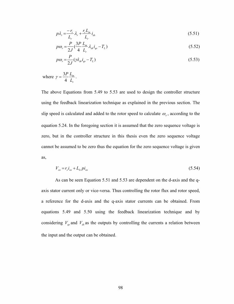
dsr
mrr
r
rr i
LLr
Lrp +
−= λλ (5.51)
)4
3(2 Lqsdr
r
mr Ti
LLP
JPp −= λω (5.52)
)(2 Lqsdrr TiJPp −= γλω (5.53)
where r
m
LLP
43
=γ .
The above Equations from 5.49 to 5.53 are used to design the controller structure
using the feedback linearization technique as explained in the previous section. The
slip speed is calculated and added to the rotor speed to calculate eω , according to the
equation 5.24. In the foregoing section it is assumed that the zero sequence voltage is
zero, but in the controller structure in this thesis even the zero sequence voltage
cannot be assumed to be zero thus the equation for the zero sequence voltage is given
as,
V (5.54) oslsossos piLir +=
As can be seen Equation 5.51 and 5.53 are dependent on the d-axis and the q-
axis stator current only or vice-versa. Thus controlling the rotor flux and rotor speed,
a reference for the d-axis and the q-axis stator currents can be obtained. From
equations 5.49 and 5.50 using the feedback linearization technique and by
considering and as the outputs by controlling the currents a relation between
the input and the output can be obtained.
qsV dsV
98

iqs*
ids*
+
+
-
-
PI
PI
Vqs
Vds
iqs
ids
Eqtn(5.49)
Eqtn(5.50)
+ - PI*rω
rω
Eqtn(5.52)
+ -PI Eqtn(5.51)
*rλ
rλ
rpω
rpλ
qspi
dspi
Figure 5.4: Control Diagram for the induction machine using feedback linearization technique. Thus the control structure for the entire machine can be summarized as,
controlling rotor speed and flux the reference for the stator currents is obtained, which
in turn are controlled to get the reference q and d- axis voltages, these voltages when
applied to the inverter synthesize the desired performance quantities. The control
scheme for the induction machine part is as shown in Figure 5.4.
As can be seen from Figure 5.4, the outputs of the controller are
rrdsqs pandppipi ωλ, . The controller transfer function is that of a PI controller
which is skk i
p + . The input-output relation for one of the controller is derived and for
the rest it is generalized.
qsi
pqsqs pIskkII =+− ))(*( 1
1 ⇒11
211
*ip
ip
qs
qs
KpKpKpK
ii
++
+= (5.55)
99
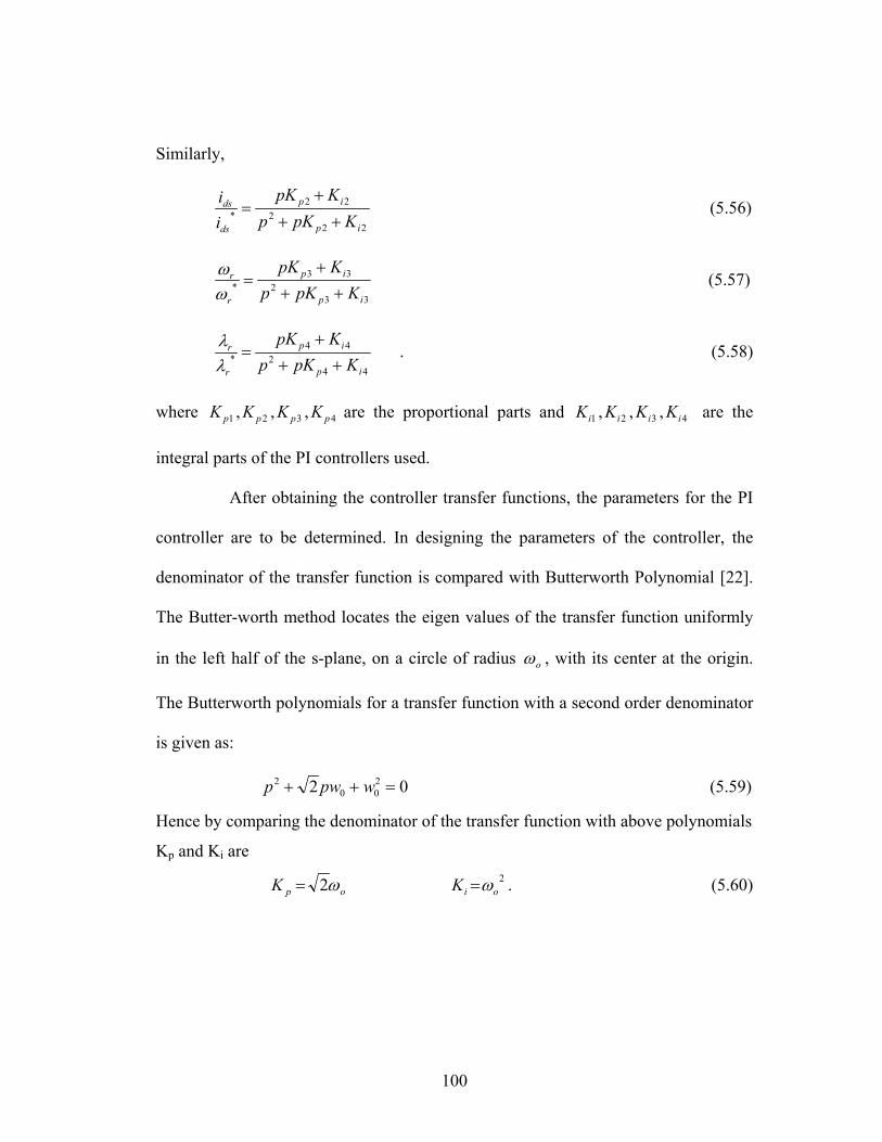
Similarly,
22
222
*ip
ip
ds
ds
KpKpKpK
ii
++
+= (5.56)
33
233
*ip
ip
r
r
KpKpKpK++
+=
ωω (5.57)
44
244
*ip
ip
r
r
KpKpKpK++
+=
λλ . (5.58)
where are the proportional parts and are the
integral parts of the PI controllers used.
4321 ,,, pppp KKKK 4321 ,,, iiii KKKK
After obtaining the controller transfer functions, the parameters for the PI
controller are to be determined. In designing the parameters of the controller, the
denominator of the transfer function is compared with Butterworth Polynomial [22].
The Butter-worth method locates the eigen values of the transfer function uniformly
in the left half of the s-plane, on a circle of radius oω , with its center at the origin.
The Butterworth polynomials for a transfer function with a second order denominator
is given as:
02 200
2 =++ wpwp (5.59)
Hence by comparing the denominator of the transfer function with above polynomials
Kp and Ki are
opK ω2= . (5.60) 2oiK ω=
100
Thus for the other controllers conditions similar to the one given above, for
the PI parameters are obtained.
In this chapter a detailed analysis of the control scheme and the controller
structure for the induction machine are give, with appropriate derivations. The
concept of vector control for induction machine has been introduced. The feedback
linearization technique for controller design has been given, and finally the
parameters for the controller using the Butterworth polynomial have been discussed.
101