Chapter 5 02user.engineering.uiowa.edu/.../Chapter_5/Chapter_5_2005.pdf · 2005-08-16 · 57:020...

57:020 Mechanics of Fluids and Transport Processes Chapter 5 Professor Fred Stern Typed by Stephanie Schrader Fall 2005 1

Chapter 5 Mass, Bernoulli, and Energy Equations 5.1 Flow Rate and Conservation of Mass 1. cross-sectional area oriented normal to velocity vector

(simple case where V ⊥ A)

U = constant: Q = volume flux = UA [m/s × m2 = m3/s] U ≠ constant: Q = ∫

AUdA

Similarly the mass flux = ∫ρ=A

UdAm

2. general case

∫ θ=

∫ ⋅=

CS

CS

dAcosV

dAnVQ

( )∫ ⋅ρ=CS

dAnVm


average velocity: AQV =

Example: At low velocities the flow through a long circular tube, i.e. pipe, has a parabolic velocity distribution (actually paraboloid of revolution).

⎟⎟⎠

⎞⎜⎜⎝

⎛⎟⎠⎞

⎜⎝⎛−=

2

max Rr1uu

i.e., centerline velocity

a) find Q and V

∫=∫ ⋅=AA

udAdAnVQ

∫ ∫ ∫ θ=π

A

2

0

R

0drrd)r(uudA

= ∫πR

0rdr)r(u2

dA = 2πrdr

u = u(r) and not θ ∴ ∫ π=θπ2

02d


Q = ∫ ⎟⎟⎠

⎞⎜⎜⎝

⎛⎟⎠⎞

⎜⎝⎛−π

R

0

2

max rdrRr1u2 = 2

max Ru21

π

maxu21V =

Continuity Equation RTT can be used to obtain an integral relationship expressing conservation of mass by defining the extensive property B = M such that β = 1. B = M = mass β = dB/dM = 1 General Form of Continuity Equation

∫ ∫ ⋅ρ+ρ==CV CS

dAVVddtd0

dtdM

or

∫ρ−=⋅∫ρCVCS

VddtddAV

net rate of outflow rate of decrease of of mass across CS mass within CV Simplifications:


1. Steady flow: 0Vddtd

CV=∫ρ−

2. V = constant over discrete dA (flow sections):

∫ ∑ ⋅ρ=⋅ρCS CS

AVdAV

3. Incompressible fluid (ρ = constant)

CS CV

dV dA dVdt

⋅ = −∫ ∫ conservation of volume

4. Steady One-Dimensional Flow in a Conduit:

∑ =⋅ρCS

0AV

−ρ1V1A1 + ρ2V2A2 = 0 for ρ = constant Q1 = Q2

Some useful definitions: Mass flux ∫ ⋅ρ=

AdAVm

Volume flux ∫ ⋅=

AdAVQ

Average Velocity A/QV =


Average Density ∫ρ=ρ dAA1

Note: m Q≠ ρ unless ρ = constant

Example

*Steady flow

*V1,2,3 = 50 fps

*@ V varies linearly from zero at wall to Vmax at pipe center *find 4m , Q4, Vmax

0 *water, ρw = 1.94 slug/ft3

∫ρ−=∫ =⋅ρCVCS

Vddtd0dAV

i.e., -ρ1V1A1 - ρ2V2A2 + ρ3V3A3 + ρ ∫4A

44dAV = 0

ρ = const. = 1.94 lb-s2 /ft4 = 1.94 slug/ft3

∫ρ= 444 dAVm = ρV(A1 + A2 – A3) V1=V2=V3=V=50f/s

= ( )222 5.1214

50144

94.1−+

π××

= 1.45 slugs/s

4m


Q4 = 75.m4 =ρ ft3/s = ∫

4A44dAV

velocity profile

Q4 = ∫ ∫ θ⎟⎟⎠

⎞⎜⎜⎝

⎛−

πor

0

2

0 omax drrd

rr1V

max

2o

2omax

r

0o

3r

0

2

max

r

0 o

2

max

r

0 omax

Vr31

31

21rV2

r3r

2rV2

drrrrV2

rdrrr1V2

o0

o

o

π=⎥⎦⎤

⎢⎣⎡ −π=

⎥⎥⎦

⎤

⎢⎢⎣

⎡−π=

∫ ⎥⎦

⎤⎢⎣

⎡−π=

∫ ⎟⎟⎠

⎞⎜⎜⎝

⎛−π=

Vmax = 86.2r

31

Q2

o

4 =π

fps

V4 ≠ V4(θ) dA4

2o

max2o

4r

Vr31

AQV

π

π==

= maxV31


5.2 Mechanical Energy, Efficiency, Bernoulli Equations, Application, and Limitations Assume irrotational, inviscid, and incompressible flow = ideal flow theory Also, assume steady flow Ω = ∇ × V = 0 ⇒ V = ∇ϕ irrotational a = − ∇(p/ρ + gz), ∇ ⋅ V = 0 inviscid, incompressible 0 a = V ⋅∇V = ∇½V ⋅ V + V × (∇ × V) steady

= ∇½V2 V2 = V ⋅ V

⎟⎠

⎞⎜⎝

⎛+

ρ−∇=∇ gzpV

21 2

0gzpV21 2 =⎟

⎠

⎞⎜⎝

⎛+

ρ+∇

i.e., p + ½ρV2 + γz = B = constant p1 + ½ρV1

2 + γz1 = p2 + ½ρV22 + γz2

Also, from continuity and irrotational

∇ ⋅ V = 0 V = ∇ϕ = kz

jy

ix ∂

ϕ∂+

∂ϕ∂

+∂ϕ∂

∇ ⋅ ∇ϕ = 0 ϕ = velocity potential


∇2ϕ = 0 i.e., governing differential equation for ϕ is Laplace equation

Application of Bernoulli’s Equation Stagnation Tube at V = 0

2Vp

2Vp

22

2

21

1 ρ+=ρ+ z1 = z2

( )122

1 pp2V −ρ

= ( )dpdp

2

1

+γ=γ=

= ( )γρ2

g2V1 =

V2 = 0 gage

Limited by length of tube and need for free surface reference


Pitot Tube 0

2

222

1

211 z

g2Vpz

g2Vp

++γ

=++γ

at at 2/1

22

11

2 zpzpg2V⎭⎬⎫

⎩⎨⎧

⎥⎦

⎤⎢⎣

⎡⎟⎠

⎞⎜⎝

⎛+

γ−⎟

⎠

⎞⎜⎝

⎛+

γ= V1 = 0

h1 h2 h = piezometric head

( )212 hhg2VV −== h1 – h2 from manometer or pressure gage

for gas flow zp∆>>

γ∆

ρ∆

=p2V


5.3 Derivation of the Energy Equation The First Law of Thermodynamics The difference between the heat added to a system and the work done by a system depends only on the initial and final states of the system; that is, depends only on the change in energy E: principle of conservation of energy ∆E = Q – W ∆E = change in energy Q = heat added to the system W = work done by the system E = Eu + Ek + Ep = total energy of the system potential energy kinetic energy The differential form of the first law of thermodynamics expresses the rate of change of E with respect to time

WQdtdE

−=

rate of work being done by system

rate of heat transfer to system

Internal energy due to molecular motion


Energy Equation for Fluid Flow The energy equation for fluid flow is derived from Reynolds transport theorem with Bsystem = E = total energy of the system (extensive property) β = E/mass = e = energy per unit mass (intensive property) = u + ek + ep

∫ ⋅ρ+∫ ρ= CSCV dAVeVeddtd

dtdE

∫ ⋅++ρ∫ +++ρ=− CS pkCV pk dAV)eeu(Vd)eeu(dtdWQ

This can be put in a more useable form by noting the following:

2V

M2/MV

massVvelocitywithmassofKETotale

22

k =∆

∆==

gzVzV

ME

e pp =

∆ρ∆γ

=∆

= (for Ep due to gravity only)

∫ ⋅⎟⎟⎠

⎞⎜⎜⎝

⎛++ρ∫ +⎟⎟

⎠

⎞⎜⎜⎝

⎛++ρ=− Cs

2

CV

2dAVugz

2VVdugz

2V

dtdWQ

rate of work rate of change flux of energy done by system of energy in CV out of CV (ie, across CS) rate of heat transfer to sysem

VV2 =


System at time t + ∆t

System at time t

CS

Rate of Work Components: fs WWW += For convenience of analysis, work is divided into shaft work Ws and flow work Wf Wf = net work done on the surroundings as a result of

normal and tangential stresses acting at the control surfaces

= Wf pressure + Wf shear Ws = any other work transferred to the surroundings

usually in the form of a shaft which either takes energy out of the system (turbine) or puts energy into the system (pump)

Flow work due to pressure forces Wf p (for system)

Work = force × distance

at 2 W2 = p2A2 × V2∆t rate of work⇒ 2222222 AVpVApW ⋅==

at 1 W1 = −p1A1 × V1∆t 1111 AVpW ⋅=

Note: here V uniform over A

(on surroundings)

neg. sign since pressure force on surrounding fluid acts in a direction opposite to the motion of the system boundary

CV


In general, AVpWfp ⋅= for more than one control surface and V not necessarily uniform over A:

∫ ⋅⎟⎠

⎞⎜⎝

⎛ρ

ρ=∫ ⋅= CSCSfp dAVpdAVpW

fshearfpf WWW += Basic form of energy equation

∫ ⋅⎟⎟⎠

⎞⎜⎜⎝

⎛++ρ+∫ ⎟⎟

⎠

⎞⎜⎜⎝

⎛++ρ=

∫ ⋅⎟⎠

⎞⎜⎝

⎛ρ

ρ−−−

CS

2

CV

2

CSfshears

dAVugz2

VVdugz2

Vdtd

dAVpWWQ

∫ ⋅⎟⎟⎠

⎞⎜⎜⎝

⎛ρ

+++ρ+

∫ ⎟⎟⎠

⎞⎜⎜⎝

⎛++ρ=−−

CS

2

CV

2

fshears

dAVpugz2

V

Vdugz2

VdtdWWQ

h=enthalpy

Usually this term can be eliminated by proper choice of CV, i.e. CS normal to flow lines. Also, at fixed boundaries the velocity is zero (no slip condition) and no shear stress flow work is done. Not included or discussed in text!


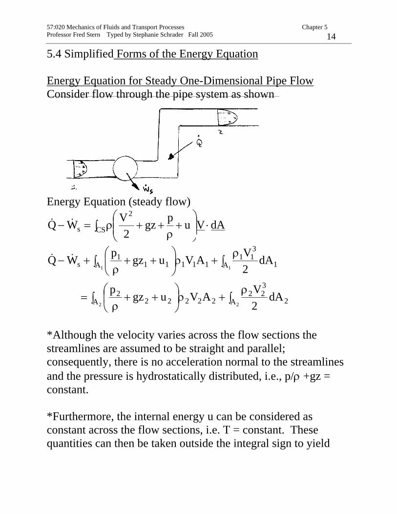
5.4 Simplified Forms of the Energy Equation Energy Equation for Steady One-Dimensional Pipe Flow Consider flow through the pipe system as shown Energy Equation (steady flow)

∫ ⋅⎟⎟⎠

⎞⎜⎜⎝

⎛+

ρ++ρ=− CS

2

s dAVupgz2

VWQ

∫ ∫ρ

+ρ⎟⎠

⎞⎜⎝

⎛++

ρ=

∫ ∫ρ

+ρ⎟⎠

⎞⎜⎝

⎛++

ρ+−

2 2

1 1

A A 2

322

222222

A A 1

311

111111

s

dA2VAVugzp

dA2VAVugzpWQ

*Although the velocity varies across the flow sections the streamlines are assumed to be straight and parallel; consequently, there is no acceleration normal to the streamlines and the pressure is hydrostatically distributed, i.e., p/ρ +gz = constant. *Furthermore, the internal energy u can be considered as constant across the flow sections, i.e. T = constant. These quantities can then be taken outside the integral sign to yield


∫ρ+∫ρ⎟⎠

⎞⎜⎝

⎛++

ρ=

∫ρ+∫ρ⎟⎠

⎞⎜⎝

⎛++

ρ+−

22

11

A 2

32

A 22222

A 1

31

A 11111

s

dA2

VdAVugzp

dA2

VdAVugzpWQ

Recall that AVdAVQ =∫ ⋅= So that mAVdAV =ρ=∫ ⋅ρ mass flow rate

Define: m2

V2

AVdA2

V 23

A

3α=

ρα=∫ρ

K.E. flux K.E. flux for V= V =constant across pipe

i.e., ∫ ⎟⎠⎞

⎜⎝⎛=α

A

3

dAVV

A1 = kinetic energy correction factor

m2

Vugzpm2

VugzpWQ22

2222

21

1111

⎟⎟⎠

⎞⎜⎜⎝

⎛α+++

ρ=⎟

⎟⎠

⎞⎜⎜⎝

⎛α+++

ρ+−

( )2

Vugzp2

VugzpWQm1 2

2222

221

1111 α+++

ρ=α+++

ρ+−

note that: α = 1 if V is constant across the flow section

α > 1 if V is nonuniform

laminar flow α = 2 turbulent flow α = 1.05 ∼ 1 may

be used


Shaft Work Shaft work is usually the result of a turbine or a pump in the flow system. When a fluid passes through a turbine, the fluid is doing shaft work on the surroundings; on the other hand, a pump does work on the fluid pts WWW −= where tW and pW are

magnitudes of power ⎟⎠⎞

⎜⎝⎛

timework

Using this result in the energy equation and deviding by g results in

gmQ

guu

2Vzp

gmW

2Vzp

gmW 12

22

222t

21

111p −

−+α++

γ+=α++

γ+

mechanical part thermal part Note: each term has dimensions of length Define the following:

QW

QgW

gmW

h pppp γ

=ρ

==

gmWh t

t =

lossheadgm

Qg

uuh 12L =−

−=


Head Loss In a general fluid system a certain amount of mechanical energy is converted to thermal energy due to viscous action. This effect results in an increase in the fluid internal energy. Also, some heat will be generated through energy dissipation and be lost (i.e. -Q). Therefore the term from 2nd law

0mgQ

guuh 12

L >−−

=

Note that adding Q to system will not make hL = 0 since this also increases ∆u. It can be shown from 2nd law of thermodynamics that hL > 0. Drop ⎯ over V and understand that V in energy equation refers to average velocity. Using the above definitions in the energy equation results in (steady 1-D incompressible flow)

Lt2

22

22

p1

21

11 hhz

g2Vphz

g2Vp

+++α+γ

=++α+γ

form of energy equation used for this course!

represents a loss in mechanical energy due to viscous stresses


Comparison of Energy Equation and Bernoulli Equation: Apply energy equation to a stream tube without any shaft work

Energy eq : L2

222

1

211 hz

g2Vpz

g2Vp

+++γ

=++γ

•If hL = 0 (i.e., µ = 0) we get Bernoulli equation and conservation of mechanical energy along a streamline •Therefore, energy equation for steady 1-D pipe flow can be interpreted as a modified Bernoulli equation to include viscous effects (hL) and shaft work (hp or ht)

Infinitesimal stream tube ⇒ α1=α2=1


abrupt change due to hp or ht

g2V

DLf

2

5.5 Concept of Hydraulic and Energy Grade Lines

Lt2

22

22

p1

21

11 hhz

g2Vphz

g2Vp

+++α+γ

=++α+γ

Define HGL = zp+

γ

EGL = g2

Vzp 2α++

γ

HGL corresponds to pressure tap measurement + z EGL corresponds to stagnation tube measurement + z

pressure tap: hp2 =γ

stagnation tube: hg2

Vp 222 =α+

γ

EGL1 + hp = EGL2 + ht + hL EGL2 = EGL1 + hp − ht − hL

point-by-point application is graphically displayed

h = height of fluid in tap/tube

EGL = HGL if V = 0

hL = g2

2VDLf

i.e., linear variation in L for D, V, and f constant

EGL1 = EGL2 + hL for hp = ht = 0

f = friction factor f = f(Re)


Helpful hints for drawing HGL and EGL 1. EGL = HGL + αV2/2g = HGL for V = 0

2.&3. g2

VDLfh

2

L = in pipe means EGL and HGL will slope

downward, except for abrupt changes due to ht or hp

Lhg2

22V

2z2p

g2

21V

1z1p+++

γ=++

γ

HGL2 = EGL1 - hL

g2

2V

Lh = for abrupt expansion


⇒

4. p = 0 ⇒ HGL = z

5. for g2

VDLfh

2

L = = constant × L

EGL/HGL slope downward

6. for change in D ⇒ change in V

i.e. V1A1 = V2A2

4DV

4DV

22

2

21

1π

=π

221

211 DVDV =

i.e., linearly increased for increasing L with

slope Vf 2

change in distance between HGL & EGL and slope change due to change in hL


7. If HGL < z then p/γ < 0 i.e., cavitation possible

condition for cavitation:

2va mN2000pp ==

gage pressure 2atmatmAg,va mN000,100pppp −=−≈−=

m10p g,va −≈γ

9810 N/m3


heat add

Neglected in text presentation

Summary of the Energy Equation The energy equation is derived from Reynolds Transport Theorem with B = E = total energy of the system β = e = E/M = energy per unit mass

= u + 2V21 +gz

internal KE PE

WQdAVeVeddtd

dtdE

CSCV−=∫ ⋅ρ+∫ρ=

vps WWWW ++=

( )∫ ⋅ρρ∫ =⋅=CSCV

p dAVpdAVpW

pts WWW −=

work done

from 1st Law of Thermodynamics

shaft work done on or by system (pump or turbine)

pressure work done

on CS

Viscous stress work on CS


mechanical energy Thermal energy

Note: each term has

units of length

V is average velocity (vector dropped) and corrected by α

( )∫ ⋅+ρ+∫ρ=+−CSCV

pt dAVepeVeddtdWWQ

gzV21ue 2 ++=

For steady 1-D pipe flow (one inlet and one outlet): 1) Streamlines are straight and parallel

⇒ p/ρ +gz = constant across CS 2) T = constant ⇒ u = constant across CS

3) define ∫ ⎟⎠⎞

⎜⎝⎛=α

CS

3

dAVV

A1 = KE correction factor

⇒ ∫ α=ρ

α=ρ m

2VA

2VdAV

2

233

Lt2

22

22

p1

21

11 hhz

g2Vphz

g2Vp

+++α+γ

=++α+γ

gmWh pp =

gmWh tt =

=−−

=gm

Qg

uuh 12L head loss

> 0 represents loss in mechanical energy due to viscosity

Chapter 5 02user.engineering.uiowa.edu/.../Chapter_5/Chapter_5_2005.pdf · 2005-08-16 · 57:020...

Documents

Transcript of Chapter 5 02user.engineering.uiowa.edu/.../Chapter_5/Chapter_5_2005.pdf · 2005-08-16 · 57:020...