Chapter 4Filter Design Techniques
149
Chapter 4 Filter Design Techniques • 7.0 Introduction • 7.1 Design of Discrete-Time IIR Filters From Continuous-Time Filters • 7.2 Design of FIR Filters by Windowing • 7.3 Examples of FIR Filters Design by the Kaiser Window Method • 7.4 Optimum Approximations of FIR Filters • 7.5 Examples of FIR Equiripple A ppro ximation • 7.6 Comments on IIR and FIR Discrete-Time Filters 1
-
Upload
kalalala01 -
Category
Documents
-
view
216 -
download
0
Transcript of Chapter 4Filter Design Techniques

8/2/2019 Chapter 4Filter Design Techniques
http://slidepdf.com/reader/full/chapter-4filter-design-techniques 1/149
Chapter 4 Filter Design Techniques
• 7.0 Introduction
• 7.1 Design of Discrete-Time IIR Filters FromContinuous-Time Filters
• 7.2 Design of FIR Filters by Windowing
• 7.3 Examples of FIR Filters Design by the KaiserWindow Method
• 7.4 Optimum Approximations of FIR Filters
• 7.5 Examples of FIR Equiripple Approximation
• 7.6 Comments on IIR and FIR Discrete-TimeFilters
1

8/2/2019 Chapter 4Filter Design Techniques
http://slidepdf.com/reader/full/chapter-4filter-design-techniques 2/149
Filter Design Techniques
7.0 Introduction
2

8/2/2019 Chapter 4Filter Design Techniques
http://slidepdf.com/reader/full/chapter-4filter-design-techniques 3/149
Introduction
• Frequency-selective filters pass only certain
frequencies
• Any discrete-time system that modifies certain
frequencies is called a filter.
• We concetrate on design of causal Frequency-
selective filters
3

8/2/2019 Chapter 4Filter Design Techniques
http://slidepdf.com/reader/full/chapter-4filter-design-techniques 4/149
Stages of Filter Design• The specification of the desired properties of the
system.
• The approximation of the specifications using a
causal discrete-time system.
• The realization of the system.
• Our focus is on second step
• Specifications are typically given in the frequency
domain.
4

8/2/2019 Chapter 4Filter Design Techniques
http://slidepdf.com/reader/full/chapter-4filter-design-techniques 5/149
Frequency-Selective Filters
• Ideal lowpass filter
ww
wwe H
c
c jw
lp,0
,1
5
0cw
cw 2 2
jwe H
1
nn
nwnh clp ,sin
8/2/2019 Chapter 4Filter Design Techniques
http://slidepdf.com/reader/full/chapter-4filter-design-techniques 6/149
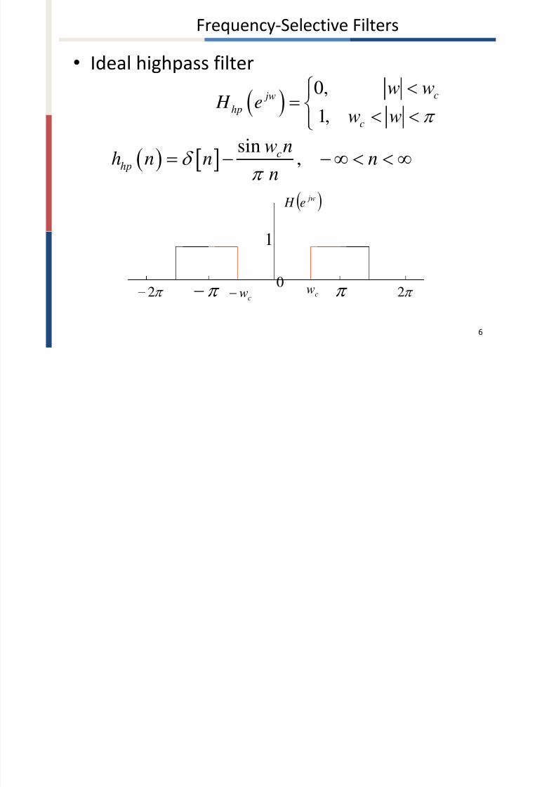
Frequency-Selective Filters
• Ideal highpass filter
0,
1,
c jw
hp
c
w w H e
w w
0
6
cwcw 2 2
jwe H
1
sin
,c
hp
w n
h n n nn

8/2/2019 Chapter 4Filter Design Techniques
http://slidepdf.com/reader/full/chapter-4filter-design-techniques 7/149
Frequency-Selective Filters
•
Ideal bandpass filter
others
wwwe H cc jw
bp,0
,121
0
7
1cw1cw
jwe H
1
2cw2cw

8/2/2019 Chapter 4Filter Design Techniques
http://slidepdf.com/reader/full/chapter-4filter-design-techniques 8/149
Frequency-Selective Filters
•
Ideal bandstop filter
others
wwwe H cc jw
bs,1
,021
0
8
1cw1cw
jwe H
1
2cw2cw

8/2/2019 Chapter 4Filter Design Techniques
http://slidepdf.com/reader/full/chapter-4filter-design-techniques 9/149
• If input is bandlimited and sampling frequency is
high enough to avoid aliasing, then overall systembehave as a continuous-time system:
T
T e H j H
T j
eff
,0
,
9
Linear time-invariant discrete-time system
,eff
jw w
H H j wT e
continuous-time specifications are converted to discretetime specifications by:
T w

8/2/2019 Chapter 4Filter Design Techniques
http://slidepdf.com/reader/full/chapter-4filter-design-techniques 10/149
Example 7.1 Determining Specifications for a
Discrete-Time Filter
•
Specifications of the continuous-time filter:• 1. passband
• 2. stopband
20002001.0101.01 for j H eff
30002001.0 for j H eff
10
sT 410
max12 22
2 5000
f T T
T
T e H j H
T j
eff
,0
,

8/2/2019 Chapter 4Filter Design Techniques
http://slidepdf.com/reader/full/chapter-4filter-design-techniques 11/149
Example 7.1 Determining Specifications for a
Discrete-Time Filter
•
Specifications of the continuous-time filter:• 1. passband
• 2. stopband
20002001.0101.01 for j H eff
30002001.0 for j H eff
11
sT 410
max12 22
2 5000
f T T
1 0.01
2 0.001
2 (2000) p
2 (3000)s

8/2/2019 Chapter 4Filter Design Techniques
http://slidepdf.com/reader/full/chapter-4filter-design-techniques 12/149
Example 7.1 Determining Specifications for a Discrete-
Time FiltersT 410
T
12
Specifications of the
discrete-time filter in
1 0.01
20.001
2 (2000) p 2 (3000)s
0.4 p 0.6s

8/2/2019 Chapter 4Filter Design Techniques
http://slidepdf.com/reader/full/chapter-4filter-design-techniques 13/149
Filter Design Constraints• Designing IIR filters is to find the approximation by a
rational function of z.
• The poles of the system function must lie inside the
unit circle(stability, causality).
• Designing FIR filters is to find the polynomial
approximation.
• FIR filters are often required to be linear-phase.
13

8/2/2019 Chapter 4Filter Design Techniques
http://slidepdf.com/reader/full/chapter-4filter-design-techniques 14/149
Filter Design Techniques
7.1 Design of Discrete-Time IIR Filters
From Continuous-Time Filters
14

8/2/2019 Chapter 4Filter Design Techniques
http://slidepdf.com/reader/full/chapter-4filter-design-techniques 15/149
7.1 Design of Discrete-Time IIR Filters From Continuous-
Time Filters
• The traditional approach to the design of
discrete-time IIR filters involves the
transformation of a continuous-time filter into a
discrete filter meeting prescribed specification.
15

8/2/2019 Chapter 4Filter Design Techniques
http://slidepdf.com/reader/full/chapter-4filter-design-techniques 16/149
Three Reasons
1. The art of continuous-time IIR filter design is
highly advanced, and since useful results can
be achieved, it is advantageous to use the
design procedures already developed for
continuous-time filters.
16

8/2/2019 Chapter 4Filter Design Techniques
http://slidepdf.com/reader/full/chapter-4filter-design-techniques 17/149
Three Reasons
2. Many useful continuous-time IIR designmethod have relatively simple closed form
design formulas. Therefore, discrete-time IIR
filter design methods based on such standardcontinuous-time design formulas are rather
simple to carry out.
17

8/2/2019 Chapter 4Filter Design Techniques
http://slidepdf.com/reader/full/chapter-4filter-design-techniques 18/149
Three Reasons
3. The standard approximation methods that
work well for continuous-time IIR filters do
not lead to simple closed-form designformulas when these methods are applied
directly to the discrete-time IIR case.
18

8/2/2019 Chapter 4Filter Design Techniques
http://slidepdf.com/reader/full/chapter-4filter-design-techniques 19/149
Steps of DT filter design by transforming a prototype
continuous-time filter
• The specifications for the continuous-time filterare obtained by a transformation of thespecifications for the desired discrete-time filter.
•
Find the system function of the continuous-timefilter.
• Transform the continuous-time filter to derivethe system function of the discrete-time filter.
19

8/2/2019 Chapter 4Filter Design Techniques
http://slidepdf.com/reader/full/chapter-4filter-design-techniques 20/149
Constraints of Transformation
• to preserve the essential properties of the
frequency response, the imaginary axis of the s-plane is mapped onto the unit circle of the z-
plane. jwe z js
20
planes plane z Im Im
Re Re

8/2/2019 Chapter 4Filter Design Techniques
http://slidepdf.com/reader/full/chapter-4filter-design-techniques 21/149
Constraints of Transformation
• In order to preserve the property of stability, If
the continuous system has poles only in the
let half of the s-plane, then the discrete-time
filter must have poles only inside the unitcircle.
21
planes Im
Re
plane z Im
Re

8/2/2019 Chapter 4Filter Design Techniques
http://slidepdf.com/reader/full/chapter-4filter-design-techniques 22/149
7.1.1 Filter Design by Impulse
Invariance•
The impulse response of discrete-time system isdefined by sampling the impulse response of a
continuous-time system.
d cd nT hT nh
22
d c T j H if ,0
w
T w j H e H then
d
c
jw ,
w for T w d
k d d
c
jwk
T j
T
w j H e H
2Relationship of frequencies

8/2/2019 Chapter 4Filter Design Techniques
http://slidepdf.com/reader/full/chapter-4filter-design-techniques 23/149
23
,, d T
relation between frequencies
S plane Z plane
-
3 / d
T
j
/ d T
/ d
T
k d d
c jw k
T j
T w j H e H 2Relationship of
frequencies
d c T j H if ,0
w
T
w j H e H then
d
c
jw ,

8/2/2019 Chapter 4Filter Design Techniques
http://slidepdf.com/reader/full/chapter-4filter-design-techniques 24/149
Aliasing in the Impulse Invariance
24
k d d
c
jwk
T
j
T
w j H e H
2
d c T j H if ,0
, jw
c
d
wthen H e H j
T
w

8/2/2019 Chapter 4Filter Design Techniques
http://slidepdf.com/reader/full/chapter-4filter-design-techniques 25/149
periodic sampling
[ ] ( ) | ( )c t nT c x n x t x nT
25
T:sample period; fs=1/T:sample rateΩs=2π/T:sample rate
n
nT t t s
s c c c
n n
x t x t s t x t t nT x nT t nT
Review
8/2/2019 Chapter 4Filter Design Techniques
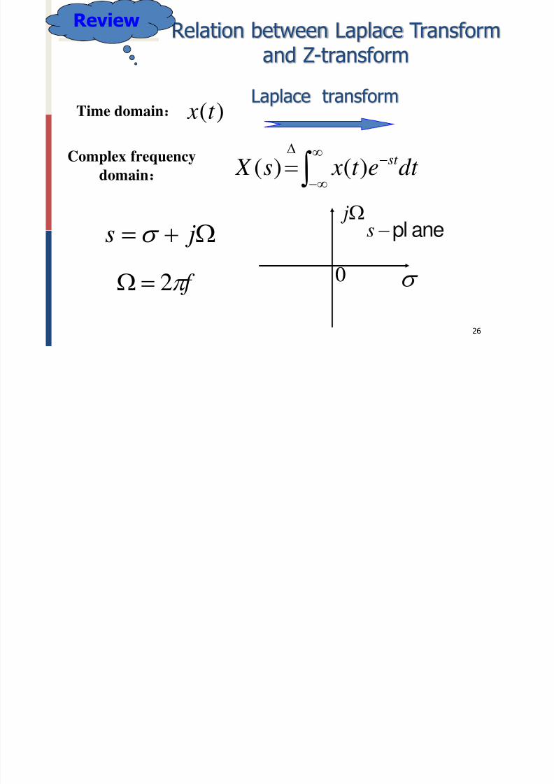
http://slidepdf.com/reader/full/chapter-4filter-design-techniques 26/149
26
Time domain: )(t x
Complex frequency
domain:
dt et xs X st )()(
Laplace transform
js
f 2
s pl ane
j
0
Relation between Laplace Transformand Z-transform
Review

8/2/2019 Chapter 4Filter Design Techniques
http://slidepdf.com/reader/full/chapter-4filter-design-techniques 27/149
27
dt et x j X t j)()(
Fourier Transform
frequency domain :
s- pl ane
j
0
Fourier Transform is the Laplace transform when s
have the value only in imaginary axis, s=jΩ
js Since
So 0 s j
dt et xs X st )()(
8/2/2019 Chapter 4Filter Design Techniques
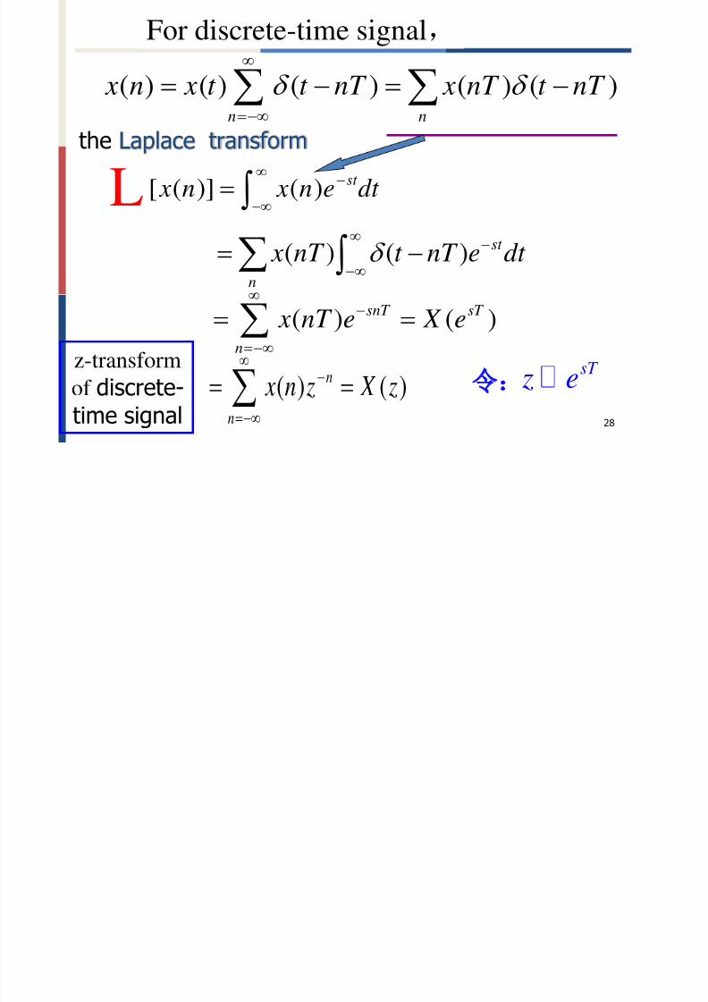
http://slidepdf.com/reader/full/chapter-4filter-design-techniques 28/149
28
( ) ( ) ( ) ( ) ( )n n
x n x t t nT x nT t nT
For discrete-time signal,
( ) ( ) st
n
x nT t nT e dt
( ) ( )snT sT
n
x nT e X e
[ ( )] ( ) st x n x n e dt
L
sT z e: ( ) ( )
n
n
x n z X z
z-transform
of discrete-
time signal
the Laplace transform

8/2/2019 Chapter 4Filter Design Techniques
http://slidepdf.com/reader/full/chapter-4filter-design-techniques 29/149
29
( )sT j T T j T j z e e e e re
n
n zn x z X )()(
so:
T r e
T
relation between
s zand
Laplace transform continuous time signal
z-transform discrete-time signalrelation
[ ( )] ( ) ( )snT sT
n
x n x nT e X e
L
sT z elet:
( )sT j T T j T j

8/2/2019 Chapter 4Filter Design Techniques
http://slidepdf.com/reader/full/chapter-4filter-design-techniques 30/149
30
2s
T f f
DTFT :
Discrete Time
Fourier Transform
( )sT j T T j T j z e e e e re
( ) ( )
j j n
n X e x n e
S plane Z plane
-
3 / s
T
j
/ s
T
/ s
T
1| j j
r z re e

8/2/2019 Chapter 4Filter Design Techniques
http://slidepdf.com/reader/full/chapter-4filter-design-techniques 31/149
31
2 2s sT f f f
zplane
Re[ ] z
Im[ ] z
0
r
0 2 / 2
0 2
2
s
s s
s s
f
f
: 0
0 2
2 4
:
s f f f
j
s pl ane
0
22
s
s
f T
sT
3
sT
3
sT
di i fil d i b i l i i

8/2/2019 Chapter 4Filter Design Techniques
http://slidepdf.com/reader/full/chapter-4filter-design-techniques 32/149
• If input is bandlimited and f s>2f max , :
d cd nT hT nh
T T e H j H
T j
eff
,0
,
32
discrete-time filter design by impulse invariance
w for T w d
k d d
c
jwk
T
j
T
w j H e H
2
d c T j H if ,0
, jw
cd
wthen H e H j w
T
l i b f i

8/2/2019 Chapter 4Filter Design Techniques
http://slidepdf.com/reader/full/chapter-4filter-design-techniques 33/149
33
,, d T
relation between frequencies
S plane Z plane
-
3 / d
T
j
/ d T
/ d
T
k d d
c jw k
T j
T w j H e H 2Relationship of
frequencies
d c T j H if ,0
w
T
w j H e H then
d
c
jw ,
i

8/2/2019 Chapter 4Filter Design Techniques
http://slidepdf.com/reader/full/chapter-4filter-design-techniques 34/149
periodic sampling
[ ] ( ) | ( )c t nT c
x n x t x nT
1 1 2*
2 2s c c s
k
X j X j S j X j k d T
34
T:sample period; fs=1/T:sample rate
Ωs=2π/T:sample rate
n
nT t t s
s c c c
n n
x t x t s t x t t nT x nT t nT
2
s
k S j k T
1
c s
k X j k T
Review
2
R i

8/2/2019 Chapter 4Filter Design Techniques
http://slidepdf.com/reader/full/chapter-4filter-design-techniques 35/149
proof of
35
T:sample period; fs=1/T:sample rate;Ωs=2π/T:sample rate
n nT t t s
2s
k
S j k T
Review
2s
k
S j k T
s jk t
k n a e
s(t)为冲击串序列,周期为T,可展开傅立叶级数
1s jk t
neT
2 ( )s jk t F
se k
2

8/2/2019 Chapter 4Filter Design Techniques
http://slidepdf.com/reader/full/chapter-4filter-design-techniques 36/149
periodic sampling
36
s c c c
n n
x t x t s t x t t nT x nT t nT
j Tn
c
k
x nT e
( ) j t
s c
n
X j x nT t nT e dt
[ ] ( ) | ( )c t nT c
x n x t x nT ( ) j j n
cn
X e x nT e
( ) ( ) ( )
j j T
s T X j X e X e
1( ) j T c s
k
X e X j k T
1 2
( ) c
k
j k X X j
T T T
e
2s
T
( ) 0, j T i f X eT
1( ) c
jthen X X j
T T
e
1
s c s
k
X j X j k T
di t ti filt d i b i l i i

8/2/2019 Chapter 4Filter Design Techniques
http://slidepdf.com/reader/full/chapter-4filter-design-techniques 37/149
[ ] ( ) | ( )c t nT c x n x t x nT
d cd nT hT nh
37
discrete-time filter design by impulse invariance
k d d
c
jwk
T
j
T
w j H e H
2
d c T j H if ,0
, jw
cd
wthen H e H j w
T
1 2( ) c
k
j k X X j
T T T e
1( ) c
j X X j
T T e
1 2
( ) c
k
j k
H H jT T T e
1
( ) c
j
H H jT T e
[ ] ( )ch n h nT

8/2/2019 Chapter 4Filter Design Techniques
http://slidepdf.com/reader/full/chapter-4filter-design-techniques 38/149
Steps of DT filter design by transforming a prototype
continuous-time filter
• Obtain the specifications for continuous-time
filter by transforming the specifications for the
desired discrete-time filter.• Find the system function of the continuous-time
filter.
• Transform the continuous-time filter to derivethe system function of the discrete-time filter.
38
8/2/2019 Chapter 4Filter Design Techniques
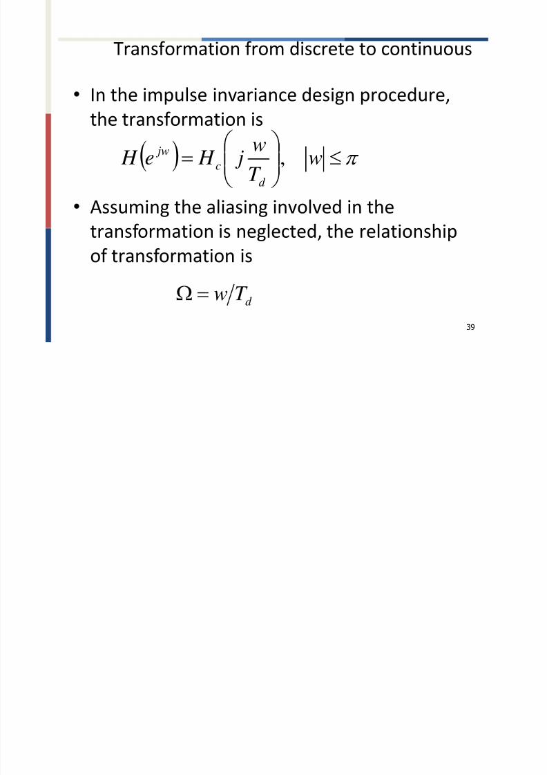
http://slidepdf.com/reader/full/chapter-4filter-design-techniques 39/149
Transformation from discrete to continuous
• In the impulse invariance design procedure,
the transformation is
• Assuming the aliasing involved in the
transformation is neglected, the relationship
of transformation is
39
wT
w
j H e H d
c
jw
,
d T w

8/2/2019 Chapter 4Filter Design Techniques
http://slidepdf.com/reader/full/chapter-4filter-design-techniques 40/149
Steps of DT filter design by transforming a prototype
continuous-time filter
• Obtain the specifications for continuous-time
filter by transforming the specifications for the
desired discrete-time filter.
• Find the system function of the continuous-time
filter.
• Transform the continuous-time filter to derive
the system function of the discrete-time filter.
40

8/2/2019 Chapter 4Filter Design Techniques
http://slidepdf.com/reader/full/chapter-4filter-design-techniques 41/149
Continuous-time IIR filters
• Butterworth filters
• Chebyshev Type I filters
•Chebyshev Type II filters
• Elliptic filters
41

8/2/2019 Chapter 4Filter Design Techniques
http://slidepdf.com/reader/full/chapter-4filter-design-techniques 42/149
Steps of DT filter design by transforming a prototype
continuous-time filter
• Obtain the specifications for continuous-time
filter by transforming the specifications for the
desired discrete-time filter.
• Find the system function of the continuous-time
filter.
•
Transform the continuous-time filter to derivethe system function of the discrete-time filter.
42

8/2/2019 Chapter 4Filter Design Techniques
http://slidepdf.com/reader/full/chapter-4filter-design-techniques 43/149
Transformation from continuous to discrete
43
N
k k
k
ss
As H
1
0,0
0,1
t
t e At h
N
k
t sk
c
k
: k d s T
k pole s s z e
two requirements for transformation
N
k
nT s
k d
N
k
nT sk d cd nue AT nue AT t hT nh d k d k
11
N
k T s
k d
ze
AT z H
d k 1 11

8/2/2019 Chapter 4Filter Design Techniques
http://slidepdf.com/reader/full/chapter-4filter-design-techniques 44/149
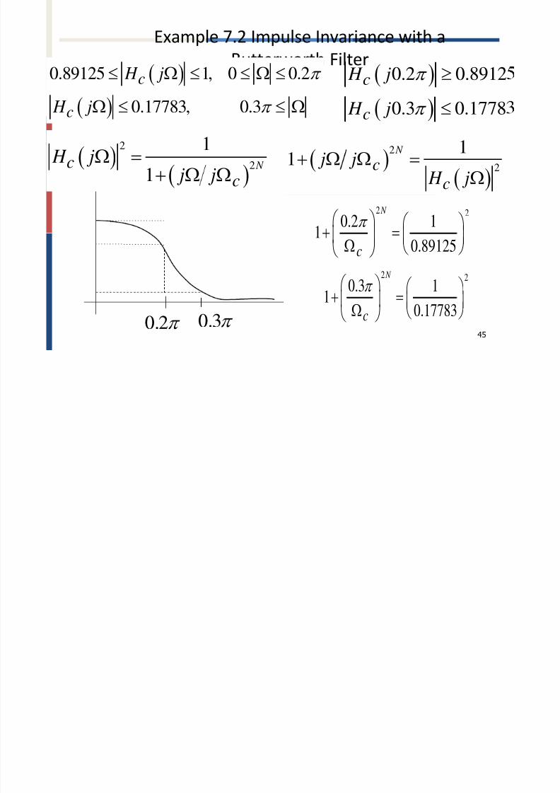
Example 7.2 Impulse Invariance with a
Butterworth Filter
•
Specifications for the discrete-time filter:
44
we H
we H
jw
jw
3.0,17783.0
2.00,189125.0
d d T wT let 1
Assume the effect of aliasing is negligible
3.0,17783.0
2.00,189125.0
j H
j H
c
c
8/2/2019 Chapter 4Filter Design Techniques
http://slidepdf.com/reader/full/chapter-4filter-design-techniques 45/149
Example 7.2 Impulse Invariance with a
Butterworth Filter
45
0.89125 1, 0 0.2
0.17783, 0.3c
c
H j
H j
0.2 0.8912
0.3 0.1778c
c
H j
H j
0.3 0.2
2 20.2 1
1
0.89125
N
c
2 2
0.3 11
0.17783
N
c
2
2
1
1 N c c
H j j j
2
2
1
1
N
cc j j H j

8/2/2019 Chapter 4Filter Design Techniques
http://slidepdf.com/reader/full/chapter-4filter-design-techniques 46/149
Example 7.2 Impulse Invariance with a
Butterworth Filter
46
2
21
1N c
c
H j j j
22
0.2 11 1.258930.89125
N
c
7032.0,6 c N
2
20.3 11 31.62204
0.17783
N
c
2
0.2 0.25893
N
c
2
0.3 30.62204
N
c
2
3 118.263782
N
70470.0,8858.5 c N
0.2 0.89125
0.3 0.17783
c
c
H j
H j
l l h

8/2/2019 Chapter 4Filter Design Techniques
http://slidepdf.com/reader/full/chapter-4filter-design-techniques 47/149
Example 7.2 Impulse Invariance with a
Butterworth Filter
2
2
1
1 N c
c H j j j
47
2
2
1
1 N c c c
c H s H s H s
s j
0,1, , 2 1k N 2 2 11 21 ,
k
j N k N N
c cs j e
6, 0.7032c N
0.182 0.679, j 0.497 0.497, j
0.679 0.182 j
Plole pairs: c H s
8/2/2019 Chapter 4Filter Design Techniques
http://slidepdf.com/reader/full/chapter-4filter-design-techniques 48/149
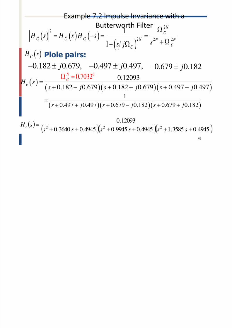
Example 7.2 Impulse Invariance with a
Butterworth Filter
48
4945.03585.14945.09945.04945.03640.0
12093.0222
ssssss
s H c
22
2 2 2
1
1
N
N N N
c
cc c c
c H s H s H s ss j
0.182 0.679, j
0.497 0.497, j
0.679 0.182 j
Plole pairs: c H s
0.12093
0.182 0.679 0.182 0.679 0.497 0.497c
H ss j s j s j
1
0.497 0.497 0.679 0.182 0.679 0.182s j s j s j
60.7032 N
c

8/2/2019 Chapter 4Filter Design Techniques
http://slidepdf.com/reader/full/chapter-4filter-design-techniques 49/149
Example 7.2 Impulse Invariance with a
Butterworth Filter
1d T
49
1 1
1 2 1 2
1
1 2
0.2871 0.4466 2.1428 1.1455
1 1.2971 0.6949 1 1.0691 0.3699
1.8557 0.6303
1 0.9972 0.2570
z z
z z z z
z
z z
0.12093
0.182 0.679 0.182 0.679 0.497 0.497c H s s j s j s j
1
0.497 0.497 0.679 0.182 0.679 0.182s j s j s j
1
N
k
k k
As s
1 1
1 11 1
N N d k k
k k k d k s T s
T A A H z
e z e z

8/2/2019 Chapter 4Filter Design Techniques
http://slidepdf.com/reader/full/chapter-4filter-design-techniques 50/149
Basic for Impulse Invariance• To chose an impulse response for the discrete-
time filter that is similar in some sense to theimpulse response of the continuous-time filter.
• If the continuous-time filter is bandlimited, thenthe discrete-time filter frequency response will
closely approximate the continuous-timefrequency response.
• The relationship between continuous-time anddiscrete-time frequency is linear; consequently,
except for aliasing, the shape of the frequencyresponse is preserved.
50

8/2/2019 Chapter 4Filter Design Techniques
http://slidepdf.com/reader/full/chapter-4filter-design-techniques 51/149
7.1.2 Bilinear Transformation
51
Bilinear transformation can avoid the
problem of aliasing.
Bilinear transformation maps
onto
w
1
1
2 1
1d
c z
H z H T z
1
1
1
12
z
z
T s
d
Bilinear transformation:
c H s
1
1
1
12
z
z
T s
d

8/2/2019 Chapter 4Filter Design Techniques
http://slidepdf.com/reader/full/chapter-4filter-design-techniques 52/149
7.1.2 Bilinear Transformation
1
1
1
12
z
z
T sd
52
sT
sT
z d
d
21
21
js 221
221
d d
d d
T jT
T jT z
any for z 10
any for z 10
1 12 (1 ) 1d T s z z
11 2 ] 1 2d d T s z T s

8/2/2019 Chapter 4Filter Design Techniques
http://slidepdf.com/reader/full/chapter-4filter-design-techniques 53/149
7.1.2 Bilinear Transformation
jsaxis j
53
2121
d
d
T jT j z
1 z 1 21 2
d
d
jw j T j T
e
planes Im
Re
plane z Im
Re
221
221
d d
d d
T jT
T jT
z
any for z 10
any for z 10
js

8/2/2019 Chapter 4Filter Design Techniques
http://slidepdf.com/reader/full/chapter-4filter-design-techniques 54/149
7.1.2 Bilinear Transformation
1
1
1
12
z
z
T
sd
54
2 1
1d
jw
jw j
T
e
e
2
tan 2d
j wT
2 2 sin 2
2cos 2d
j w
T w
2tan
2w
T d
2tan2 1
d T w
/2 /2 /2
/2 /2 /2
2 ( )
( )d
jw jw jw
jw jw jwT
e e e
e e e
relation between frequency response of Hc(s), H(z)

8/2/2019 Chapter 4Filter Design Techniques
http://slidepdf.com/reader/full/chapter-4filter-design-techniques 55/149
55
2tan
2
2tan
2
:
s
d s
p
d p
T
T
prewarp
2tan
2)()(
d T
c j j H e H
q y p c( ), ( )
Comments on the Bilinear Transformation

8/2/2019 Chapter 4Filter Design Techniques
http://slidepdf.com/reader/full/chapter-4filter-design-techniques 56/149
Comments on the Bilinear Transformation
• It avoids the problem of aliasing encountered
with the use of impulse invariance.
• It is nonlinear compression of frequency axis.
56
S plane Z plane
-
3 / d
T
j
/ d
T
/ d
T
2tan2 wT d
2tan21
d T w
Comments on the Bilinear Transformation

8/2/2019 Chapter 4Filter Design Techniques
http://slidepdf.com/reader/full/chapter-4filter-design-techniques 57/149
Comments on the Bilinear Transformation
• The design of discrete-time filters using bilinear
transformation is useful only when this
compression can be tolerated or compensated for,
as the case of filters that approximate ideal
piecewise-constant magnitude-responsecharacteristics.
57
0cw
cw
2 2
jwe H
1
Bilinear Transformation ofs
e

8/2/2019 Chapter 4Filter Design Techniques
http://slidepdf.com/reader/full/chapter-4filter-design-techniques 58/149
Bilinear Transformation of
58
1
1
1
12
z
z
T
sd
2tan2
w
T d
e j
e
2tan 2
d
wT
d T

8/2/2019 Chapter 4Filter Design Techniques
http://slidepdf.com/reader/full/chapter-4filter-design-techniques 59/149
Comparisons of Impulse Invariance and Bilinear
Transformation
• The use of bilinear transformation is restricted tothe design of approximations to filters with
piecewise-constant frequency magnitude
characteristics, such as highpass, lowpass andbandpass filters.
• Impulse invariance can also design lowpass filters.
However, it cannot be used to design highpassfilters because they are not bandlimited.
59

8/2/2019 Chapter 4Filter Design Techniques
http://slidepdf.com/reader/full/chapter-4filter-design-techniques 60/149
Comparisons of Impulse Invariance and Bilinear
Transformation
• Bilinear transformation cannot design filter
whose magnitude response isn’t piecewise
constant, such as differentiator. However,Impulse invariance can design an bandlimited
differentiator.
60

8/2/2019 Chapter 4Filter Design Techniques
http://slidepdf.com/reader/full/chapter-4filter-design-techniques 61/149
• Butterworth Filter,
•
Chebyshev Approximation,• Elliptic Approximation
61
7.1.3 Example of Bilinear
Transformation
we H
we H
jw
jw
6.0,001.0
4.0,01.199.0
xamp e . near

8/2/2019 Chapter 4Filter Design Techniques
http://slidepdf.com/reader/full/chapter-4filter-design-techniques 62/149
pTransformation of a Butterworth
Filter
0.89125 1, 0 0.2
0.17783, 0.3
jw
jw
H e w
H e w
620.0160.01
2 0.20.89125 1, 0 tan
2
2 0.30.7783, tan
2
c
d
c
d
H j
T
H jT
, 1d For convenience we choose T ,17783.015.0tan2
,89125.01.0tan2
j H
j H
c
c
2tan2 wT d

8/2/2019 Chapter 4Filter Design Techniques
http://slidepdf.com/reader/full/chapter-4filter-design-techniques 63/149
Example 7.3 Bilinear Transformation of a Butterworth Filter
,17783.015.0tan2
,89125.01.0tan2
j H
j H
c
c
63
N
c
c j j
j H 2
2
11
2 2
2 2
2tan 0.1 1
1 0.89125
3tan 0.15 11
0.17783
N
c
N
c
305.5 N
766.0
,6
c
N
0.0160.01

8/2/2019 Chapter 4Filter Design Techniques
http://slidepdf.com/reader/full/chapter-4filter-design-techniques 64/149
Locations of Poles
64
0,1, , 2 1k N 2 2 11 21 ,
k
j N k N N
c cs j e
0.1998 0.7401, j
0.5418 0.5418, j
0.7401 0.1998 j
Plole pairs: c H s
2
2
1
1 N c
c
H j j j
2
2
1
1
N c c c
c
H s H s H s
s j
6, 0.766c N
Examp e 7.3 Bi inear

8/2/2019 Chapter 4Filter Design Techniques
http://slidepdf.com/reader/full/chapter-4filter-design-techniques 65/149
pTransformation of a Butterworth
Filter
5871.04802.15871.00836.15871.03996.0
20238.0222
ssssss
s H c
65
21
2121
61
2155.09904.01
1
3583.00106.117051.02686.11
10007378.0
z z
z z z z
z
z H
22
2 2 2
1
1
N
N N N
c
cc c cc
H s H s H s ss j
0.1998 0.7401, j 0.5418 0.5418, j 0.7401 0.1998 j
Plole pairs: c H s
1
1
1
12
z
z
T s
d
. . time filter

8/2/2019 Chapter 4Filter Design Techniques
http://slidepdf.com/reader/full/chapter-4filter-design-techniques 66/149
time filter
66

8/2/2019 Chapter 4Filter Design Techniques
http://slidepdf.com/reader/full/chapter-4filter-design-techniques 67/149
Example 7.4 Butterworth Approximation (Hw)
67
we H
we H jw
jw
6.0,001.0
4.0,01.199.014 N order
Example 7.4 frequency response

8/2/2019 Chapter 4Filter Design Techniques
http://slidepdf.com/reader/full/chapter-4filter-design-techniques 68/149
p q y p
68
Chebyshev filters

8/2/2019 Chapter 4Filter Design Techniques
http://slidepdf.com/reader/full/chapter-4filter-design-techniques 69/149
69
y
C Chebyshev filter (type I)
) / (1
1|)(|22
2
c N
cV
j H
)coscos()( 1 x N xV N
c
1
1
Chebyshev polynomial
Chebyshev filter (type II)
122
2
)] / ([1
1|)(|
c N
cV
j H
1
c
E l 7 5 Ch b h T I II A i i

8/2/2019 Chapter 4Filter Design Techniques
http://slidepdf.com/reader/full/chapter-4filter-design-techniques 70/149
Example 7.5 Chebyshev Type I , II Approximation
70
we H we H
jw
jw
6.0,001.04.0,01.199.0 8 N order
Type I Type II
.Cheb she

8/2/2019 Chapter 4Filter Design Techniques
http://slidepdf.com/reader/full/chapter-4filter-design-techniques 71/149
Chebyshev
71
Type I Type II
elliptic filters

8/2/2019 Chapter 4Filter Design Techniques
http://slidepdf.com/reader/full/chapter-4filter-design-techniques 72/149
72
E
p f
Elliptic filter
)(1
1|)(|
22
2
N
c
U
j H
s p
1
11
2 Jacobian elliptic function

8/2/2019 Chapter 4Filter Design Techniques
http://slidepdf.com/reader/full/chapter-4filter-design-techniques 73/149
Example 7.6 Elliptic Approximation
73
we H
we H
jw
jw
6.0,001.0
4.0,01.199.0
6 N order
.Elliptic

8/2/2019 Chapter 4Filter Design Techniques
http://slidepdf.com/reader/full/chapter-4filter-design-techniques 74/149
Elliptic
74
*Comparison of Butterworth, Chebyshev, elliptic filters: Example

8/2/2019 Chapter 4Filter Design Techniques
http://slidepdf.com/reader/full/chapter-4filter-design-techniques 75/149
75
p f , y , p f p
-Given specification
0.4|| .011 |)(| 99.0 je H
||0.6 0.001 |)(| j
e H
6.0 ,4.0 001.0 ,01.0 s21 p
)( s
-Order
Butterworth Filter : N=14. ( max flat)
Chebyshev Filter : N=8. ( Cheby 1, Cheby 2)Elliptic Filter : N=6 ( equiripple)
B
C
E
-Pole-zero plot (analog)

8/2/2019 Chapter 4Filter Design Techniques
http://slidepdf.com/reader/full/chapter-4filter-design-techniques 76/149
76
p ( g)
-Pole-zero plot (digital)
B C1 C2 E
B C1 C2 E
(14) (8)

8/2/2019 Chapter 4Filter Design Techniques
http://slidepdf.com/reader/full/chapter-4filter-design-techniques 77/149
77
-Magnitude -Group delay
B
C1
C2
E
B
C1
C2
E
4.0 6.0 4.0 6.0
5
20

8/2/2019 Chapter 4Filter Design Techniques
http://slidepdf.com/reader/full/chapter-4filter-design-techniques 78/149
7.2 Design of FIR Filters by Windowing
•FIR filters are designed based on directlyapproximating the desired frequency response
of the discrete-time system.
•
Most techniques for approximating themagnitude response of an FIR system assume a
linear phase constraint.
78

8/2/2019 Chapter 4Filter Design Techniques
http://slidepdf.com/reader/full/chapter-4filter-design-techniques 79/149
Window Method• An ideal desired frequency response
79
n
jwn
d
jw
d enhe H
dwee H nh jwn jw
d d 2
1
Many idealized systems are defined by
piecewise-constant frequency response withdiscontinuities at the boundaries. As a result,these systems have impulse responses that
are noncausal and infinitely long.
ww
wwe H
c
c jwlp
,0
,1
sinc
lp
w nh n
n
0cw
cw
jw
e H 1

8/2/2019 Chapter 4Filter Design Techniques
http://slidepdf.com/reader/full/chapter-4filter-design-techniques 80/149
Window Method
80
otherwise
M nnhnh
d
,0
0,
nwnhnh d
otherwise
M n
nw ,0
0,1
d eW e H e H w j jw
d
jw
2
1
The most straightforward approach toobtaining a causal FIR approximation is totruncate the ideal impulse response.
Windowing in Frequency Domain

8/2/2019 Chapter 4Filter Design Techniques
http://slidepdf.com/reader/full/chapter-4filter-design-techniques 81/149
• Windowed frequency response
81
deWeH21eH j j
d j
The windowed version is smeared version
of desired response
Window Method

8/2/2019 Chapter 4Filter Design Techniques
http://slidepdf.com/reader/full/chapter-4filter-design-techniques 82/149
82
1
2
j w jw j jw
d d H e H e W e d H e
If nnw 1
k n
jwn jwk wenweW 22
0cw
cw
jwe H
1
0 5 10510 1515
2
2
2 4 4 6
jwW e
h f d

8/2/2019 Chapter 4Filter Design Techniques
http://slidepdf.com/reader/full/chapter-4filter-design-techniques 83/149
Choice of Window• is as short as possible in duration. This
minimizes computation in the implementation of the filter.
83
nw
approximates an impulse. jweW
0
M jw jwn jwn
n n
W e w n e e
1
2sin 1 21
1 sin 2
jw M
jwM
jw
w M ee
e w
otherwise
M nnw
,0
0,1
1 M
2
1 M
2
1 M
jwW e
d h d

8/2/2019 Chapter 4Filter Design Techniques
http://slidepdf.com/reader/full/chapter-4filter-design-techniques 84/149
Window Method
84
jw
d
w j jw
d
jw e H d eW e H e H
21
then would look like , exceptwhere changes very abruptly.
jwe H jw
d e H
jw
d e H
nw jweW
0w
If is chosen so that is concentrated
in a narrow band of frequencies around
0cwcw
jw
d H e
1
1 M
2
1 M
2
1 M
jwW e
R l Wi d

8/2/2019 Chapter 4Filter Design Techniques
http://slidepdf.com/reader/full/chapter-4filter-design-techniques 85/149
Rectangular Window• for the rectangular window has a
generalized linear phase.
85
jweW
As M increases, the width of the “main lobe” decreases. 4 1
mw M
While the width of each lobe decreases with
M, the peak amplitudes of the main lobe andthe side lobes grow such that the area undereach lobe is a constant.
2sin 1 2
sin 2
jw jwM w M
W e ew
1 M
2
1 M
2
1 M
1
M
M
1
M
M
R l Wi d

8/2/2019 Chapter 4Filter Design Techniques
http://slidepdf.com/reader/full/chapter-4filter-design-techniques 86/149
Rectangular Window
86
will oscillate at
the discontinuity.
d eW e H w j jw
d
The oscillations occur more rapidly, butdo not decrease in magnitude as Mincreases.
The Gibbs phenomenon can bemoderated through the use of a lessabrupt truncation of the Fourier series.
R l Wi d

8/2/2019 Chapter 4Filter Design Techniques
http://slidepdf.com/reader/full/chapter-4filter-design-techniques 87/149
Rectangular Window• By tapering the window smoothly to zero at
each end, the height of the side lobes can bediminished.
• The expense is a wider main lobe and thus a
wider transition at the discontinuity.
87
.Method

8/2/2019 Chapter 4Filter Design Techniques
http://slidepdf.com/reader/full/chapter-4filter-design-techniques 88/149
Method• To design an ilowpass FIR Filters
88
wwwwe H
c
c jw
lp,0
,1
sinc
lp
w nh n
n
0cw
cw
jwe H
1
Review
d h n h n w n
1, 0
0,
n M w n
otherwise
d eW e H e H w j jw
d
jw
2
1
1 M
2
1 M
2
1 M
jwW e
sin 2
2
cw n M
n M
02 M 0
2 M 0
M
M
2 M 0 M

8/2/2019 Chapter 4Filter Design Techniques
http://slidepdf.com/reader/full/chapter-4filter-design-techniques 89/149
7.2.1 Properties of Commonly Used Windows• Rectangular
89
otherwise
M nnw
,0
0,1
otherwise
M n M M n M n M n
nw
,0
2,2220,2
Bartlett (triangular)
7 2 1 P i f C l U d Wi d

8/2/2019 Chapter 4Filter Design Techniques
http://slidepdf.com/reader/full/chapter-4filter-design-techniques 90/149
7.2.1 Properties of Commonly Used Windows
•
Hanning
90
otherwise
M n M nnw
,0
0,2cos5.05.0
otherwise
M n M nnw
,0
0,2cos46.054.0
Hamming

8/2/2019 Chapter 4Filter Design Techniques
http://slidepdf.com/reader/full/chapter-4filter-design-techniques 91/149
7.2.1 Properties of Commonly Used Windows
• Blackman
91
otherwise
M n M n
M n
nw
,0
0,4cos08.0
2cos5.042.0

8/2/2019 Chapter 4Filter Design Techniques
http://slidepdf.com/reader/full/chapter-4filter-design-techniques 92/149
7.2.1 Properties of Commonly Used Windows
92

8/2/2019 Chapter 4Filter Design Techniques
http://slidepdf.com/reader/full/chapter-4filter-design-techniques 93/149
93
Frequency Spectrum of Windows
(a) Rectangular, (b) Bartlett,(c) Hanning, (d) Hamming,
(e) Blackman , (M=50)
(a)-(e) attenuation of sidelobe increases,
width of mainlobe increases.
7 2 1 P i f C l U d Wi d

8/2/2019 Chapter 4Filter Design Techniques
http://slidepdf.com/reader/full/chapter-4filter-design-techniques 94/149
7.2.1 Properties of Commonly Used Windows
94
biggest,high oscillations
at discontinuity
smallest,
the sharpest transition
Table 7.1
7 2 2 I i f G li d Li Ph

8/2/2019 Chapter 4Filter Design Techniques
http://slidepdf.com/reader/full/chapter-4filter-design-techniques 95/149
7.2.2 Incorporation of Generalized Linear Phase
• In designing FIR filters, it is desirable to obtain
causal systems with a generalized linear phase
response.
95
otherwise M nn M wnw
,00,
The above five windows are allsymmetric about the point ,i.e.,2 M
7 2 2 I ti f G li d Li Ph

8/2/2019 Chapter 4Filter Design Techniques
http://slidepdf.com/reader/full/chapter-4filter-design-techniques 96/149
7.2.2 Incorporation of Generalized Linear Phase
• Their Fourier transforms are of the form
96
2 M jw jw
e
jweeW eW
wof functionevenand realaiseW jw
e
causalnwnhnh d :
d d d if h M n h n h n h n w n
2 M jw jw
e
jwee Ae H
:h M n h n generalized linear phase
2 M
M

8/2/2019 Chapter 4Filter Design Techniques
http://slidepdf.com/reader/full/chapter-4filter-design-techniques 97/149
7.2.2 Incorporation of Generalized Linear Phase
phaselinear d generalizenhn M h
nwnhnhnhn M hif d d d
:
97
2 M jw jwo jw ee jAe H
2 M
M
Frequency Domain Representation

8/2/2019 Chapter 4Filter Design Techniques
http://slidepdf.com/reader/full/chapter-4filter-design-techniques 98/149
Frequency Domain Representation
98
nhn M hif d d 2 M jw jw
e
jw
d ee H e H
1
2
jw
d
j w j H e H W d e e
1
2e e
j w jw jwewhere A H W d e e e
221
2e e
j w j w M j j M H W d e e e e
2 M jw jw
e
jweeW eW
w n w M n
2 jw jwM e A e e
d h n h n w n
Example 7 7 Linear Phase Lowpass Filter

8/2/2019 Chapter 4Filter Design Techniques
http://slidepdf.com/reader/full/chapter-4filter-design-techniques 99/149
Example 7.7 Linear-Phase Lowpass Filter
• The desired frequency response is
99
ww
wwee H
c
c jwM
jw
lp,0
,2
lph M n
nw
Mn
M nwnh c
2
2sin
21
2
sin 2
2
c
clp
c
w
w
jwM jwn
h n dw
w n M for n
n M
e e
2 M
wwe H
wwe H
s
jw
p
jw01
magnitude frequency response

8/2/2019 Chapter 4Filter Design Techniques
http://slidepdf.com/reader/full/chapter-4filter-design-techniques 100/149
magnitude frequency response
100
pw
sw
1 0 jw
p p
jw
s s
H e w w
H e w w
s pw w w
1020log p p
0.1 0.15 jw
H e w
1 0.05 0 0.25 jw H e w
0.1s p
w w w 10
20log 0.05 26 p
dB
1020logs s
20s dB
7 2 1 Properties of Commonly Used Windows

8/2/2019 Chapter 4Filter Design Techniques
http://slidepdf.com/reader/full/chapter-4filter-design-techniques 101/149
7.2.1 Properties of Commonly Used Windows
101
smallest,the sharpest
transitionbiggest,high oscillations
at discontinuity
7 2 3 The Kaiser Window Filter Design Method

8/2/2019 Chapter 4Filter Design Techniques
http://slidepdf.com/reader/full/chapter-4filter-design-techniques 102/149
7.2.3 The Kaiser Window Filter Design Method
102
1 22
0
0
1, 0
0,
I nn M w n
I
otherwise
2,where M
0 : I u zero order modified Bessel function of the first kind
2
0
1
21
!r
r u I u
r
: 1,length M : parameter shape
:two parameters
Trade side-lobe amplitude for main-lobe width

8/2/2019 Chapter 4Filter Design Techniques
http://slidepdf.com/reader/full/chapter-4filter-design-techniques 103/149
103Figure 7.24
As increases, attenuation of
sidelobe increases, width of
mainlobe increases.
As M increases, attenuation of
sidelobe is preserved, width of mainlobe decreases.
M=20
(a) Window shape, M=20,
(b) Frequency spectrum, M=20,
(c) beta=6
=6
Table 7.1

8/2/2019 Chapter 4Filter Design Techniques
http://slidepdf.com/reader/full/chapter-4filter-design-techniques 104/149
104
Transition width is a little less than
mainlobe width
Comparison
8/2/2019 Chapter 4Filter Design Techniques
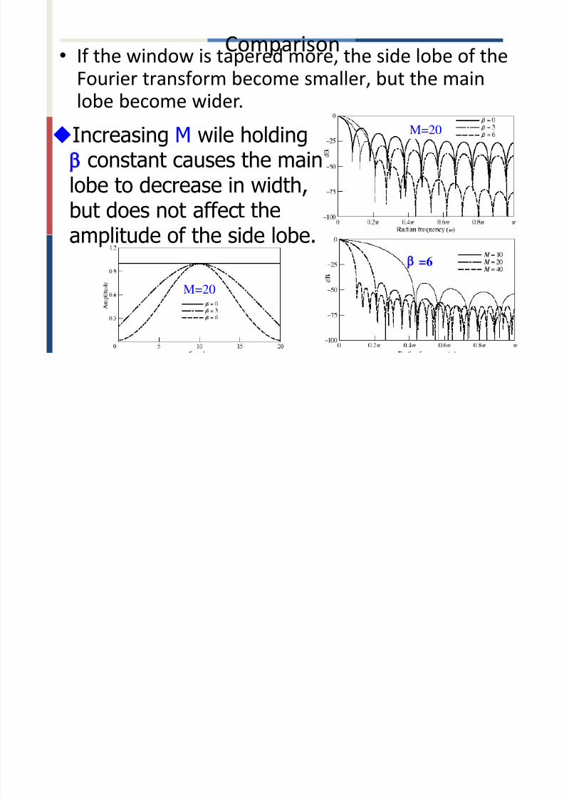
http://slidepdf.com/reader/full/chapter-4filter-design-techniques 105/149
Comparison• If the window is tapered more, the side lobe of the
Fourier transform become smaller, but the mainlobe become wider.
105
Increasing M wile holding constant causes the mainlobe to decrease in width,but does not affect theamplitude of the side lobe.
M=20
=6
M=20
Filter Design by Kaiser Window

8/2/2019 Chapter 4Filter Design Techniques
http://slidepdf.com/reader/full/chapter-4filter-design-techniques 106/149
Filter Design by Kaiser Window
106
pw
sw
wwe H
wwe H
s
jw
p
jw
01
ps www
10log20 A
Filter Design by Kaiser Window1 2

8/2/2019 Chapter 4Filter Design Techniques
http://slidepdf.com/reader/full/chapter-4filter-design-techniques 107/149
Filter Design by Kaiser Window
1 22
0
0
1
, 0
0,
I n
n M w n I
otherwise
107
ps www 10log20 A
21,0.0
5021,2107886.0215842.0
50,7.81102.04.0
A
A A A
A A
2285.2
8
w
A M M=20
Example 7.8 Kaiser Window Design of a Lowpass
Filt

8/2/2019 Chapter 4Filter Design Techniques
http://slidepdf.com/reader/full/chapter-4filter-design-techniques 108/149
Filter
we H
we H
jw
jw
6.0,001.0
4.0,01.199.0
108
ps
www 10log20 A
1 22
0
0
1
sin , 0c
I n
w n n M n I
0,
h notherwise
5.182 M where
21,0.0
5021,2107886.0215842.0
50,7.81102.04.0
A
A A A
A A
8
2.285
A M
w
Example 7.8 Kaiser Window Design of a Lowpass

8/2/2019 Chapter 4Filter Design Techniques
http://slidepdf.com/reader/full/chapter-4filter-design-techniques 109/149
p g p
Filter
we H
we H
jw
jw
6.0,001.0
4.0,01.199.0
109
001.0,min,001.0,01.0,6.0,4.0
:1
2121
s p ww
step
0.52
s p
c
w wcutoff frequency w
2 :step
3:step100.2 20log 60
0.5653 37
s pw w w A
M
Example 7.8 Kaiser Window Design of a Lowpass

8/2/2019 Chapter 4Filter Design Techniques
http://slidepdf.com/reader/full/chapter-4filter-design-techniques 110/149
Filter
2
0
1
21
!r
r u
I ur
110
0.5653
5.182 M where
1 22
0
0
1
sin , 0c
I n
w n n M n I
0,
h notherwise
21,0.0
5021,2107886.0215842.0
50,7.81102.04.0
A
A A A
A A
837
2.285
A M
w
10
3:
0.2 20log 60s p
step
w w w A
. .Filter
1 2
2
0 1sin
I nw n

8/2/2019 Chapter 4Filter Design Techniques
http://slidepdf.com/reader/full/chapter-4filter-design-techniques 111/149
111
0
0
sin, 0
cw nh n n M
n I
7.3 Examples of FIR Filters Design by the Kaiser

8/2/2019 Chapter 4Filter Design Techniques
http://slidepdf.com/reader/full/chapter-4filter-design-techniques 112/149
Window Method• The ideal highpass filter with generalized linear
phase
112
wwe
wwe H
c
M jw
c jw
hp
,
,02
jw
lp
M jw jw
hp e H ee H 2
n M n
M nw M n
M nnh chp ,
22sin
22sin
hph n h n w n
Example 7.9 Kaiser Window Design of a Highpass

8/2/2019 Chapter 4Filter Design Techniques
http://slidepdf.com/reader/full/chapter-4filter-design-techniques 113/149
Filter• Specifications:
113
wwe H
wwe H
p
jw
s
jw
,11
,
11
2
021.0,5.0,35.0 211 ps wwwhere
24,6.2 M
By Kaiser window method
Example 7.9 Kaiser Window Design of a Highpass

8/2/2019 Chapter 4Filter Design Techniques
http://slidepdf.com/reader/full/chapter-4filter-design-techniques 114/149
Filter• Specifications:
114
wwe H
wwe H
p
jw
s
jw
,11
,
11
2
021.0,5.0,35.0 211 ps wwwhere
24,6.2 M
By Kaiser window method
7.3.2 Discrete-Time Differentiator

8/2/2019 Chapter 4Filter Design Techniques
http://slidepdf.com/reader/full/chapter-4filter-design-techniques 115/149
7.3.2 Discrete Time Differentiator
115
we jwe H M jw jw
diff ,2
n
M n
M n
M n
M nnhdiff ,
2
2sin
2
2cos2
nwnhnh diff
phaselinear d generalize IV typeor III typen M hnh :
Example 7.10 Kaiser Window Design of a

8/2/2019 Chapter 4Filter Design Techniques
http://slidepdf.com/reader/full/chapter-4filter-design-techniques 116/149
Differentiator
• Since kaiser’s formulas were developed forfrequency responses with simple magnitude
discontinuities, it is not straightforward to
apply them to differentiators.
• Suppose
116
4.210 M
Group Delay

8/2/2019 Chapter 4Filter Design Techniques
http://slidepdf.com/reader/full/chapter-4filter-design-techniques 117/149
Group Delay
• Phase:
• Group Delay:
117
25
22 ww M
samples M
5
2
Group Delay

8/2/2019 Chapter 4Filter Design Techniques
http://slidepdf.com/reader/full/chapter-4filter-design-techniques 118/149
Group Delay
• Phase:
• Group Delay:
• Noninteger delay
118
225
22 ww M
samples M
2
5
2
7 4 Optimum Approximations of FIR Filters

8/2/2019 Chapter 4Filter Design Techniques
http://slidepdf.com/reader/full/chapter-4filter-design-techniques 119/149
7.4 Optimum Approximations of FIR Filters
• Goal: Design a ‘best’ filter for a given M
• In designing a causal type I linear phase FIR filter,
it is convenient first to consider the design of a
zero phase filter.
•
Then insert a delay sufficient to make it causal.
119
nhnh ee
7.4 Optimum Approximations of FIR Filters

8/2/2019 Chapter 4Filter Design Techniques
http://slidepdf.com/reader/full/chapter-4filter-design-techniques 120/149
7.4 Optimum Approximations of FIR Filters
nhnh ee
120
2, M Lenhe A L
Ln
jwn
e
jw
e
function periodicevenrealwnnhhe A
L
n
ee
jw
e ,,:cos201
.2 samples M Lbyit delaying
bynh fromobtained becansystemcausal A e
n M h M nhnh e 2
2 M jw jw
e
jwee Ae H
7 4 Optimum Approximations of FIR Filters

8/2/2019 Chapter 4Filter Design Techniques
http://slidepdf.com/reader/full/chapter-4filter-design-techniques 121/149
7.4 Optimum Approximations of FIR Filters
• Designing a filter to meet these specifications is to
find the (L+1) impulse response values
121
Lnnhe 0,
In Packs-McClellan algorithm,is fixed, and is variable.
21,,, and ww L s p
21 or
Packs-McClellan algorithm is the dominantmethod for optimum design of FIR filters.
7 4 Optimum Approximations of FIR Filters

8/2/2019 Chapter 4Filter Design Techniques
http://slidepdf.com/reader/full/chapter-4filter-design-techniques 122/149
7.4 Optimum Approximations of FIR Filters
wnwT wn n coscoscoscoscos 1
122
1coscos0coscos0cos 1
0 wwT w
wwwT w coscoscos1coscos1cos 1
1
1cos2cos2cos 22 wwT w
wT wT w
wT wn
nn
n
coscoscos2
coscos
21
wwwww
wwww
cos3cos4cos1cos2cos2
cos2coscos23cos
32
7.4 Optimum Approximations of FIR Filters

8/2/2019 Chapter 4Filter Design Techniques
http://slidepdf.com/reader/full/chapter-4filter-design-techniques 123/149
7.4 Optimum Approximations of FIR Filters
L
k
k
k
w x
L
k
k k
L
n
ee jw
e
xa xPwhere
xPwawnnhhe A
0
cos01
coscos20
123
functionweightingtheiswW where
e Ae H wW w E
functionerror ionapproximat an Define
jw
e
jw
d
7.4 Optimum Approximations of FIR Filters

8/2/2019 Chapter 4Filter Design Techniques
http://slidepdf.com/reader/full/chapter-4filter-design-techniques 124/149
7.4 Optimum Approximations of FIR Filters
124
ww
wwe H
s
p jw
d ,0
0,1
ww
wwK wW
s
p
,1
0,
1
1
2
Minimax criterion

8/2/2019 Chapter 4Filter Design Techniques
http://slidepdf.com/reader/full/chapter-4filter-design-techniques 125/149
• Within the frequency interval of the passband
and stopband, we seek a frequency responsethat minimizes the maximum weightedapproximation error of
125
jw
e e A
jw
e
jw
d e Ae H wW w E
w E
F w Lnnhe maxmin
0:
Other criterions

8/2/2019 Chapter 4Filter Design Techniques
http://slidepdf.com/reader/full/chapter-4filter-design-techniques 126/149
00:1 min dww E H
Lnnhe
126
0
2
0:2 min dww E H Lnnhe
w E H
F w Lnnhe
maxmin0:
Alternation Theorem• Let denote the closet subset consisting of theF

8/2/2019 Chapter 4Filter Design Techniques
http://slidepdf.com/reader/full/chapter-4filter-design-techniques 127/149
• Let denote the closet subset consisting of the
disjoint union of closed subsets of the real axis x.
127
pF
is an r th-order polynomial.
r
k
k
k xa xP0
denotes a given desired function of x that is continuous on
x DP
pF
is a positive function, continuous on pF xW P
The weighted error is xP x D xW x E PPP
x E E PF x P
max
The maximum error is defined as
Alternation Theorem

8/2/2019 Chapter 4Filter Design Techniques
http://slidepdf.com/reader/full/chapter-4filter-design-techniques 128/149
• A necessary and sufficient condition that be the
unique r th-order polynomial that minimizes isthat exhibit at least (r+2) alternations; i.e.,
there must exist at least (r+2) values in such
that
128
xP
E x E P
i x PF
221 r x x x
E x E x E iPiP 1
1,,2,1 r i
and such that
for
Example 7.11 Alternation Theorem and
Polynomials

8/2/2019 Chapter 4Filter Design Techniques
http://slidepdf.com/reader/full/chapter-4filter-design-techniques 129/149
Polynomials
• Each of these polynomials is of fifth order.
• The closed subsets of the real axis x referred
to in the theorem are the regions
129
11.01.01 xand x
1 xW P
7.4.1 Optimal Type I Lowpass Filters

8/2/2019 Chapter 4Filter Design Techniques
http://slidepdf.com/reader/full/chapter-4filter-design-techniques 130/149
p yp p
• For Type I lowpass filter
• The desired lowpass frequency response
•
Weighting function
130
L
k
k
k wawP0
coscos
wwww
wwwww D
ss
p p
pcoscos1,0
01coscos,1cos
wwww
wwwwK wW
ss
p p p
coscos1,1
01coscos,1
cos
7.4.1 Optimal Type I Lowpass Filters

8/2/2019 Chapter 4Filter Design Techniques
http://slidepdf.com/reader/full/chapter-4filter-design-techniques 131/149
• The weighted approximation error is
• The closed subset is
or
131
wPw DwW w E PPP coscoscoscos
wwand ww s p0
s p wwand ww cos11coscos
x E P
7.4.1 Optimal Type I Lowpass Filters

8/2/2019 Chapter 4Filter Design Techniques
http://slidepdf.com/reader/full/chapter-4filter-design-techniques 132/149
p yp p
•The alternation theorem states that a set of coefficients will correspond to the filterrepresenting the unique best approximationto the ideal lowpass filter with the ratio
fixed at K and with passband and stopbandedge and if and only if exhibits atleast (L+2) alternations on , i.e., if and onlyif alternately equals plus and minus its
maximum value at least (L+2) times.• Such approximations are called equiripple
approximations.
132
k a
21
pwsw )(cos w E P
PF
)(cos w E P
7.4.1 Optimal Type I Lowpass Filters

8/2/2019 Chapter 4Filter Design Techniques
http://slidepdf.com/reader/full/chapter-4filter-design-techniques 133/149
• The alternation theorem states that theoptimum filter must have a minimum of (L+2)
alternations, but does not exclude the
possibility of more than (L+2) alternations.• In fact, for a lowpass filter, the maximum
possible number of alternations is (L+3).
133
7.4.1 Optimal Type I Lowpass Filters

8/2/2019 Chapter 4Filter Design Techniques
http://slidepdf.com/reader/full/chapter-4filter-design-techniques 134/149
p yp p
•
Because all of the filters satisfy the alternationtheorem for L=7 and for the same value
of , it follows that and/or must be
different for each ,since the alternation
theorem states that the optimum filter under
the conditions of the theorem is unique.
134
21 K
pw sw
Property for type I lowpass filters from the
alternation theorem

8/2/2019 Chapter 4Filter Design Techniques
http://slidepdf.com/reader/full/chapter-4filter-design-techniques 135/149
alternation theorem
•
The maximum possible number of alternations of the error is (L+3)
• Alternations will always occur at and
•
All points with zero slop inside the passband andall points with zero slop inside stopband will
correspond to alternations; i.e., the filter will be
equiripple, except possibly at and
135
pw sw
0w
w
7.4.2 Optimal Type II Lowpass Filters

8/2/2019 Chapter 4Filter Design Techniques
http://slidepdf.com/reader/full/chapter-4filter-design-techniques 136/149
p yp p
• For Type II causal FIR filter:
• The filter length (M+1) is even, ie, M is odd
• Impulse response is symmetric
• The frequency response is
136
M nnh 0
nhn M h
21,,2,1,212
2
1cos
2cos2
21
1
2
21
0
2
M nn M hnbwhere
nwnbe
n M
wnhee H
M
n
M jw
M
n
M jw jw
7.4.2 Optimal Type II Lowpass Filters

8/2/2019 Chapter 4Filter Design Techniques
http://slidepdf.com/reader/full/chapter-4filter-design-techniques 137/149
21
0
21
1cos
~
2cos2
1
cos
M
n
M
nwnnbwnwnb
137
wPwee H M jw jw cos2cos2
21cos0
M Land wawPwhere L
k
k
k
n M hnbnbnba find k 212~
7.4.2 Optimal Type II Lowpass Filters

8/2/2019 Chapter 4Filter Design Techniques
http://slidepdf.com/reader/full/chapter-4filter-design-techniques 138/149
• For Type II lowpass filter,
138
ww
ww
ww De H s
p
P
jw
d
,0
0,
2cos
1
cos
ww
wwK
w
wW wW
s
pP
,2cos
0,2cos
cos
7.4.3 The Park-McClellan Algorithm

8/2/2019 Chapter 4Filter Design Techniques
http://slidepdf.com/reader/full/chapter-4filter-design-techniques 139/149
• From the alternation theorem, the optimum filter
will satisfy the set of equation
139
2,,2,111
Lie Ae H wW i jw
e
jw
d
jwe e A
ii
jw
d
jw
d
jw
d
L
L
L
L L L
L
L
w xwhere
e H
e H
e H
a
a
wW x x x
wW x x x
wW x x x
L
cos
11
11
11
2
2
1
1
0
2
2
2
2
22
2
2
2
22
1
1
2
11
7.4.3 The Park-McClellan Algorithm

8/2/2019 Chapter 4Filter Design Techniques
http://slidepdf.com/reader/full/chapter-4filter-design-techniques 140/149
•
Guessing a set of alternation frequencies
140
2
12
1
1
2
1 cos,1
1
L
k ii
ii
ik
k L
k k
k
k
L
k
jw
d k
w x x x
bwhere
wW
b
e H b k
2,,2,1 Li for wi sl pl wwww 1,and
7.4.3 The Park-McClellan Algorithm

8/2/2019 Chapter 4Filter Design Techniques
http://slidepdf.com/reader/full/chapter-4filter-design-techniques 141/149
141
2
1
1
1
1
1
1
1
cos,cos
Lk k
L
k ii ik
k
k k L
k
k k
k
L
k
k k jw
e
x xb x x
d
w x x
x xd
C x xd
wPe A
7.4.3 The Park-McClellan Algorithm

8/2/2019 Chapter 4Filter Design Techniques
http://slidepdf.com/reader/full/chapter-4filter-design-techniques 142/149
• For equiripple lowpass approximation
• Filter length: (M+1)
142
ps wwwwherew
M
324.2
13log10 2110
. xamp es o qu r pp eApproximation
7 5 1 L Fil

8/2/2019 Chapter 4Filter Design Techniques
http://slidepdf.com/reader/full/chapter-4filter-design-techniques 143/149
7.5.1 Lowpass Filter
we H
we H jw
jw
6.0,001.0
4.0,01.199.0
143
26 M
wwe Awwe A
wW w E w E
error ionapproximat unweighted
s
jw
e
p
jw
e A
,00,1
Comments

8/2/2019 Chapter 4Filter Design Techniques
http://slidepdf.com/reader/full/chapter-4filter-design-techniques 144/149
• M=26, Type I filter• The minimum number of alternations is
(L+2)=(M/2+2)=15
• 7 alternations in passband and 8 alternationsin stopband
• The maximum error in passband and
stopband are 0.0116 and 0.0016, whichexceed the specifications.
144
7.5.1 Lowpass Filter

8/2/2019 Chapter 4Filter Design Techniques
http://slidepdf.com/reader/full/chapter-4filter-design-techniques 145/149
• M=27, , Type II filter, zero at z=-1• The maximum error in passband and
stopband are 0.0092 and 0.00092, which
exceed the specifications.• The minimum number of alternations is
(L+2)=(M-1)/2+2=15
• 7 alternations in passband and 8 alternationsin stopband
145
w
Comparison

8/2/2019 Chapter 4Filter Design Techniques
http://slidepdf.com/reader/full/chapter-4filter-design-techniques 146/149
• Kaiser window method require M=38 to meetor exceed the specifications.
• Park-McClellan method require M=27
• Window method produce approximatelyequal maximum error in passband and
stopband.
• Park-McClellan method can weight the errordifferently.
146
7.6 Comments on IIR and FIR Discrete-Time
Filters

8/2/2019 Chapter 4Filter Design Techniques
http://slidepdf.com/reader/full/chapter-4filter-design-techniques 147/149
Filters
•
What type of system is best, IIR or FIR?• Why give so many different design methods?
• Which method yields the best result?
147
7.6 Comments on IIR and FIR Discrete-Time
Filters

8/2/2019 Chapter 4Filter Design Techniques
http://slidepdf.com/reader/full/chapter-4filter-design-techniques 148/149
Filters
148
Closed-Form
Formulas
GeneralizedLinear Phase
Order
IIR Yes No Low
FIR No Yes High
7.2.1 Properties of Commonly Used Windows
h f d

8/2/2019 Chapter 4Filter Design Techniques
http://slidepdf.com/reader/full/chapter-4filter-design-techniques 149/149
• Their Fourier transforms are concentrated
around• They have a simple functional form that allows
them to be computed easily.
0w
The Fourier transform of the Bartlettwindow can be expressed as a product of Fourier transforms of rectangular windows.
The Fourier transforms of the otherwindows can be expressed as sums of