Chapter 4.1 Mixture Problems -...

Special Topics

Chapter 4.1

Mixture Problems

Chapter 4: Linear Programming

Lesson Plan

Mixture Problems

Combining Resources to Maximize Profit

Finding the Optimal Production Policy

Why the Corner Point Principle Works

Decreasing-Time-List Algorithm

Linear Programming

Life Is Complicated

A Transportation Problem

Delivering Perishables

Improving on the Current Solution

Mathematical Literacy in Today’s World, 8th ed.

For All Practical Purposes


Mixture Problems

Mixture Problem

Limited resources are

combined into products

in such a way that the

profit from selling those

products is a maximum.

Linear Programming

A management science technique that helps a business

allocate the resources it has on hand to make a particular mix of

products that will maximize profit.

One of the most frequently used management science

techniques.


Mixture Problems

Production Policy

A solution to a linear-programming mixture problem is a

production policy that tells us how many units of each

product to make.

Optimal Production Policy Has Two Properties

First, it is possible; that is, it does not violate any of

the limitations under which the manufacturer

operates, such as availability of resources.

Second, the optimal production policy gives the

maximum profit.


Mixture Problems

Common Features of Mixture Problems

Resources – Available in limited, known quantities

for time period.

Products – Made by combining, or mixing, the

resources.

Recipes – How many units of each resource are

needed.

Profits – Each product earns a known profit per unit.

Objectives – To find how much of each product to

make to maximize profit without

exceeding any of the resource limitations.


Mixture Problems

Mixture Problem: Making Skateboards and Dolls

Skateboards require five units of plastic and are sold

for $1 profit.

Dolls require two units of plastic and are sold for $0.55

profit.

If 60 units of plastic are available, what numbers of

skateboards and/or dolls should be manufactured to

maximize the profits?


Mixture Problems

Step 1

Mixture Chart – display the verbal information into a

chart that includes the unknown variables (―x‖ units

of Skateboards, and ―y‖ units of dolls).


Mixture Problems

Example 2

Make a mixture chart to display this situation: A clothing

manufacturer has 60 yards of cloth available to make shirts

and decorated vests. Each shirt requires 3 yards of cloth

and provides a profit of $5. Each vest requires 2 yards of

cloth and provides a profit of $3.

Let x =

Let y =


Mixture Problems


Mixture Problems

Translating Mixture Charts into

Mathematical Form


Mixture Problems

What must be true about the sign of the numbers we can

use for ―x‖ and ―y‖ in the skateboard/doll problem?

Both ―x‖ and ―y‖ cannot be negative numbers.

How can we write this information using an inequality sign,

like >, or ≥, or <, or ≤?

x ≥ 0

y ≥ 0


Mixture Problems

These inequalities are called minimum constraints.

Which means that one cannot manufacture negative

numbers of objects.


Mixture Problems

The next problem is that we only have so much plastic

available to make skateboards and dolls.

How can we represent this information?

Since we need five units of plastic for each skateboard, we

can write that information mathematically as needing 5x

units of plastic for each skateboard.

Since we need 2 units of plastic for each doll, we can write

that information mathematically as needing 2y units of

plastic.

Hence we will need 5x + 2y units of plastic for the mixture

of skateboards and dolls we make.


Mixture Problems

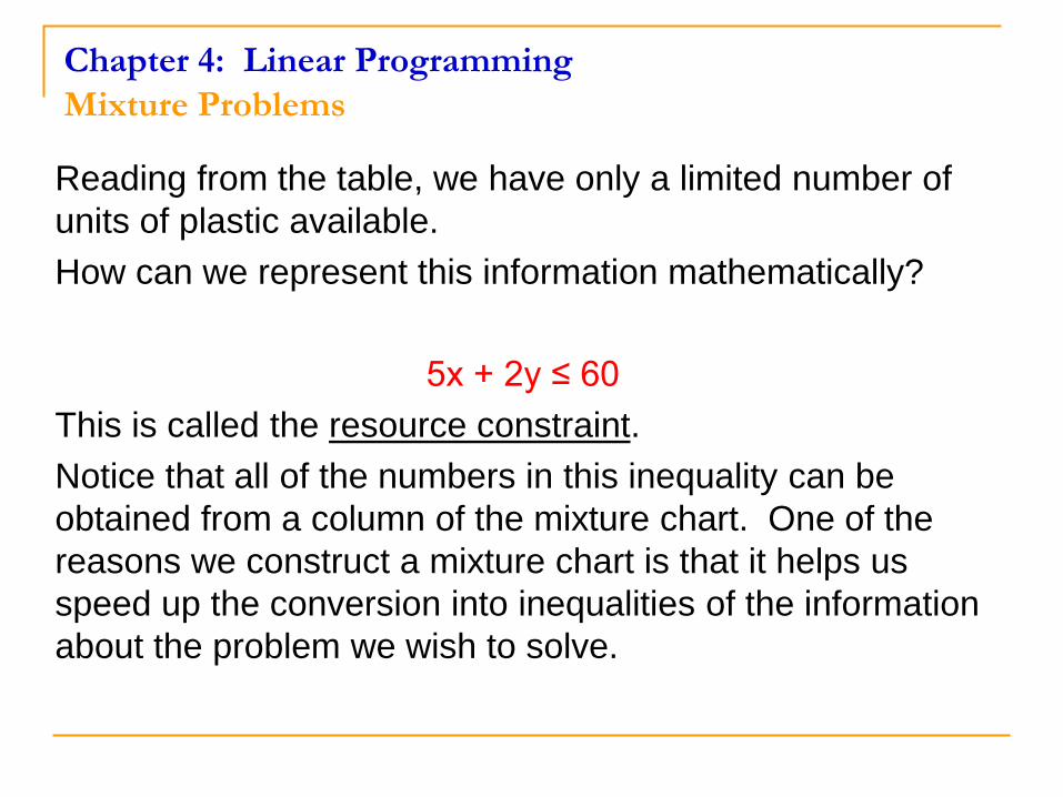
Reading from the table, we have only a limited number of

units of plastic available.

How can we represent this information mathematically?

5x + 2y ≤ 60

This is called the resource constraint.

Notice that all of the numbers in this inequality can be

obtained from a column of the mixture chart. One of the

reasons we construct a mixture chart is that it helps us

speed up the conversion into inequalities of the information

about the problem we wish to solve.


Mixture Problems

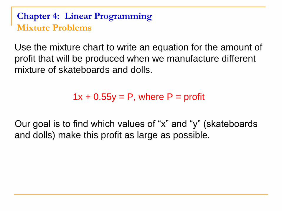
Use the mixture chart to write an equation for the amount of

profit that will be produced when we manufacture different

mixture of skateboards and dolls.

1x + 0.55y = P, where P = profit

Our goal is to find which values of ―x‖ and ―y‖ (skateboards

and dolls) make this profit as large as possible.


Mixture Problems

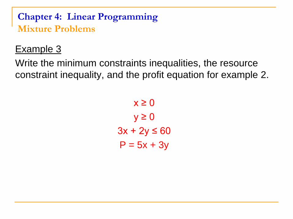
Example 3

Write the minimum constraints inequalities, the resource

constraint inequality, and the profit equation for example 2.

x ≥ 0

y ≥ 0

3x + 2y ≤ 60

P = 5x + 3y


Mixture Problems

Feasibility set (feasibility region) - A

collection of all physically possible

solutions, or choices, that can be

made.


Mixture Problems

Feasibility Set or Feasibility Region

Our goal is to find the best mixture of ―x‖ and ―y‖

(skateboards and/or dolls) to produce the largest

profit — two phases:

1. Find the feasible set for the mixture problem

subject to limited resources.

Graph line below 5x + 2y 60 (plastic)

2. Determine the mixture that gives rise to the

largest profit.


Mixture Problems

To draw the graph of an inequality, let’s first review how to

draw the graph of the equation of a straight line.

Remember that two points can be used to uniquely

determine a straight line. Let’s use the equation associated

with the resource constraint in example 1.

The resource constraint is 5x + 2y ≤ 60. The equation

associated with this inequality is

5x + 2y = 60


Mixture Problems

There are two points that are easy to find on this line.

When x = 0, this gives rise to one point on the line, and

when y = 0, we can find another point. Find these two

points.


Mixture Problems

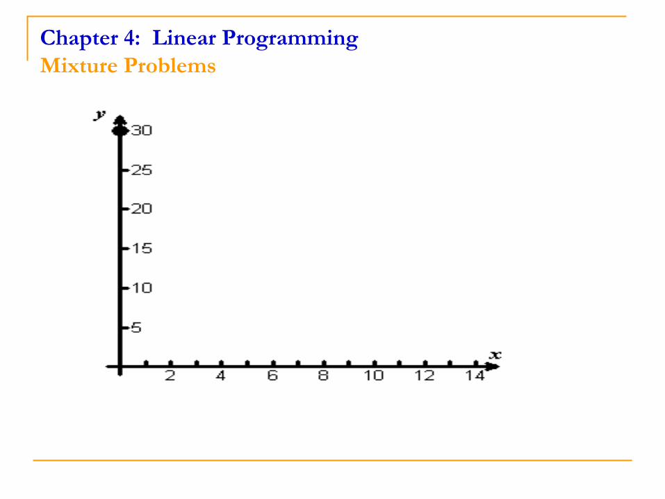
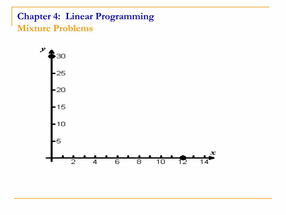
Let x = 0 so,

5(0) + 2y = 60

0 + 2y = 60

2y = 60

y = 30

The point (0, 30) is on the line.


Mixture Problems


Mixture Problems

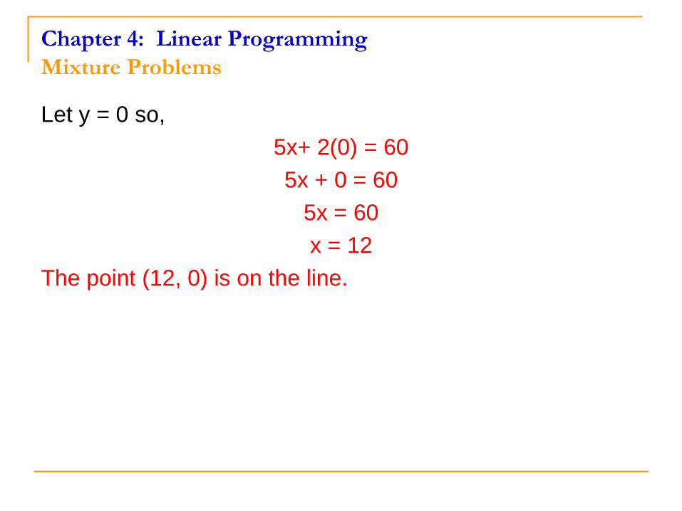
Let y = 0 so,

5x+ 2(0) = 60

5x + 0 = 60

5x = 60

x = 12

The point (12, 0) is on the line.


Mixture Problems


Mixture Problems

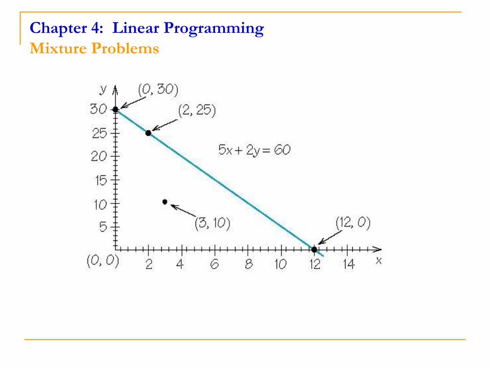
Now that we know the graph of the equation 5x + 2y = 60

looks , we can think through where points (x, y) that satisfy

5x + 2y < 60 are located. The points that are either on the

line 5x + 2y = 60 or satisfy 5x + 2y < 60 will satisfy

5x + 2y ≤ 60.

Any line, for example, 5x + 2y = 60, divides the xy-plane

into three parts: those points on the line, and the points in

one of the two half-planes. In one of the half-planes we

have the points for which 5x + 2y < 60 and in the other we

have the points for which 5x + 2y > 60.

How can we tell which of the two half-planes is above the

line 5x + 2y = 60 and which is below?


Mixture Problems

The key is the use of a test point (x, y) that is not on the line

and whose half-planes we wish to distinguish.

We saw that (3, 10) is not on the line 5x + 2y = 60 and is

below the line. This enables us to see that the half-plane

for which 5x + 2y < 60 consists of the points below the line

5x + 2y = 60.

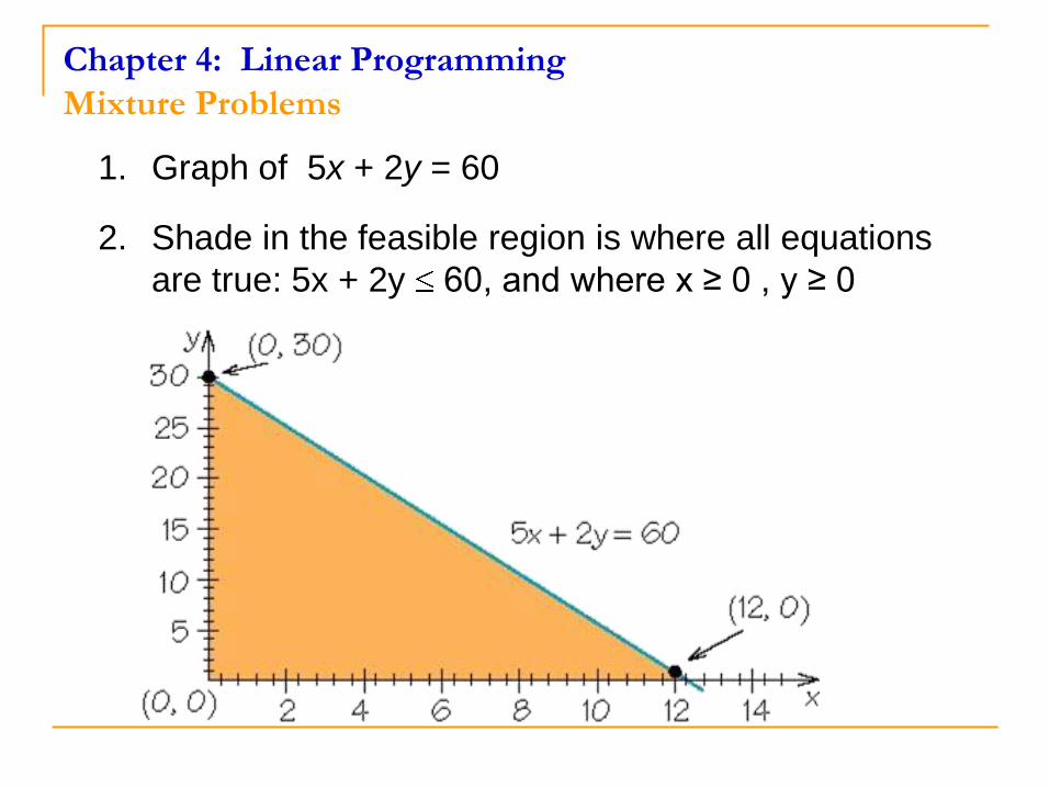
1. Graph of 5x + 2y = 60

2. Shade in the feasible region is where all equations

are true: 5x + 2y 60, and where x ≥ 0 , y ≥ 0


Mixture Problems


Mixture Problems

Example 4

In the earlier clothing manufacturer example, we developed

a resource constraint of 3x + 2y ≤ 60. Draw the feasible

region corresponding to that resource constraint, using the

reality minimums of x ≥ 0 and y ≥ 0.

1. Graph 3x + 2y = 60.

Let x = 0

0 + 2y = 60

2y = 60

y = 30

Graph (0, 30).


Mixture Problems

Let y = 0

3x + 0 = 60

3x = 60

x = 20

So graph (20, 0).

Which way are you going to shade?

Below the line 3x + 2y = 60.


Mixture Problems

AssignmentTextbook Pages 139-140 #2,4,6,12,16

Chapter 4.1 Mixture Problems -...

Documents

Transcript of Chapter 4.1 Mixture Problems -...