1

Chapter 40

Quantum Mechanics in 1-Dimension In quantum mechanics we use the “wave picture” to completely describe the behavior of a particle. Quantum mechanics allows us to find the probability of finding a particle in various regions. One surprising result is that there is a finite, nonzero probability that microscopic particles will pass through barriers, even though such a process is forbidden in Newtonian mechanics. Schrodinger Equation in 1-Dimension The notes for this section were taken from a textbook titled “Introduction to Quantum Mechanics”, chapter 2, written by David Griffiths.

In quantum mechanics we determine the particle’s “wave function” Ψ(x,t) by solving the time-dependent Schrodinger’s equation:

!!2

2m"2#(x, t)"x2

+U(x, t)#(x, t) = i! "#(x, t)"t

The initial condition is usually that the wave function is known at t = 0, i.e., we know Ψ(x,0). Here i = !1 ,

2

! = h2!

, U(x,t) is the potential energy of the particle, m is

the mass of the particle, and h is Planck’s constant. Max Born’s statistical interpretation of the wave function is that !(x, t) 2 gives the probability density of finding the particle at point x at time t. More precisely, the probability of finding the particle between x = a and x = b at time t is given by

!(x, t) 2a

b

" dx

The wave function itself is complex, but ! 2

=!*! is real and positive, as a probability should be. The statistical interpretation introduces indeterminacy into quantum mechanics. All quantum mechanics has to offer is statistical information about the possible results. The statistical interpretation of the wave function requires that the probability of finding the particle somewhere on the x-axis from x = -∞ to x = +∞ is one. That is,

!(x, t) 2"#

+#

$ dx =1

This is so because the particle has to be somewhere! This is known as the normalization condition. It turns out that

3

if the wave function Ψ(x,t) is normalized at t = 0, then it stays normalized for all future times. In this course we will consider cases where the potential energy U(x,t) of the particle is independent of time, i.e., U(x,t) → U(x). In this case we solve Schrodinger’s equation using the method of separation of variables where we look for separable solutions that are simple products of the form:

Ψ(x,t) = ψ(x) φ(t) In the end we will put together the separable solutions in such a way as to construct the most general solution to Schrodinger’s equation. Note that

!"!t

=!d"dt

!2"!x2

=d 2!dx2

"

and also note the ordinary derivatives. The Schrodinger equation then becomes

!!2

2md 2!dx2

"+U(x)!" = i!! d"dt

4

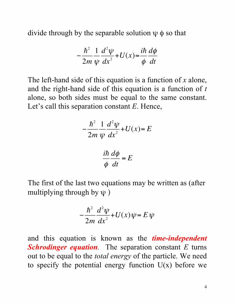
divide through by the separable solution ψ φ so that

!!2

2m1!d 2!dx2

+U(x)= i!!d!dt

The left-hand side of this equation is a function of x alone, and the right-hand side of this equation is a function of t alone, so both sides must be equal to the same constant. Let’s call this separation constant E. Hence,

!!2

2m1!d 2!dx2

+U(x)= E

i!!d!dt

= E

The first of the last two equations may be written as (after multiplying through by ψ )

!!2

2md 2!dx2

+U(x)!= E!

and this equation is known as the time-independent Schrodinger equation. The separation constant E turns out to be equal to the total energy of the particle. We need to specify the potential energy function U(x) before we

5

can solve the time-independent Schrodinger equation for ψ(x). The boundary conditions for ψ(x) are that ψ(x) and dψ/dx are continuous. The second of the two equations above may be written as

d!!= !

i!E dt

and the solution to this equation is

!(t) = e!i E!t

The separable solutions of the form Ψ(x,t) = ψ(x) φ(t) are known as stationary states, and thus take the form

!(x, t) =!(x)"(t) =!(x)e"i E!t

The separable solutions have the following properties: (1) they represent stationary states. Although the wave

function itself does depend on time

!(x, t) =!(x)e"i E!t

6

the probability density is time-independent! That is,

!(x, t) 2 =!*(x, t)!(x, t) =! *(x)e+i E!t!(x)e

"i E!t

!(x, t) 2 = !(x) 2

which is time-independent. (2) The stationary states represented by the separable solutions are states of definite total energy. A separable solution has the property that every measurement of the total energy E is certain to return the value E. (3) The general solution Ψ(x,t) to the time-dependent Schrodinger equation is a linear combination of the separable solutions. The time-independent Schrodinger’s equation yields an infinite collection of solutions

!1(x), !2 (x), !3(x),...

each with its associated value of the separation constant E1, E2, E3,…. Thus there is a different wave function for each allowed energy value:

!1(x, t) =!1(x)e"i E1!t

7

! 2 (x, t) =!2 (x)e"i E2!t

!3(x, t) =!3(x)e

"i E3!t

etc…These separable solutions represent the stationary states. Now, since the Schrodinger equation has the property that any linear combination of solutions is itself a solution, we can construct the most general solution Ψ(x,t) as a linear combination of the separable solutions:

Ψ(x,t) = C1 Ψ1(x,t) + C2 Ψ2(x,t) + C3 Ψ3(x,t) +…

!(x, t) = cnn=1

"

# ! n (x, t) = cn !n (x)e$i En!t

n=1

"

#

(4) The separable solutions ψn(x) are mutually orthogonal, in the sense that

! *n (x)

!"

"

# !m (x) dx = 0

whenever n ≠ m. Here n and m are discrete indices. Orthogonality and normalization may be combined in a single statement as

! *

n (x)!"

"

# !m (x) dx = "nm

8

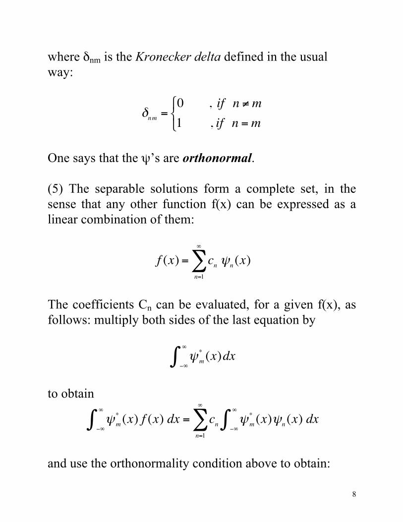
where δnm is the Kronecker delta defined in the usual way:

!nm =0 , if n !m1 , if n =m"#$

One says that the ψ’s are orthonormal. (5) The separable solutions form a complete set, in the sense that any other function f(x) can be expressed as a linear combination of them:

f (x) = cnn=1

!

" !n (x)

The coefficients Cn can be evaluated, for a given f(x), as follows: multiply both sides of the last equation by

! *m (x)

!"

"

# dx

to obtain

! *m (x)

!"

"

# f (x) dx = cnn=1

"

$ ! *m (x)

!"

"

# !n (x) dx

and use the orthonormality condition above to obtain:

9

cn = ! *n (x)

!"

"

# f (x) dx

40.2 Particle in a Box Consider a particle of mass m trapped in an ∞ well such that the potential energy of the particle is given by

U(x) =0 , if 0 ! x ! L" , otherwise#$%

A particle inside this well is completely free, except at the two ends (x = 0 and x = L), where an ∞ force prevents the particle from escaping.

Outside the well, ψ(x) = 0 since the probability of finding the particle there is zero.

10

Inside the well, where U(x) = 0, the time-independent Schrodinger equation becomes

!!2

2md 2!dx2

= E !

d 2!dx2

+2mE!2

! = 0

let

k ! 2mE!

so that

d 2!dx2

+ k 2 ! = 0

and the solution to this equation is

!(x) = Asin kx( )+Bcos kx( )

where A and B are constants fixed by the boundary conditions of the problem. In this problem only the continuity of the wave function ψ(x) applies since the potential energy goes to infinity at the walls of the well. The continuity of ψ(x) requires that

ψ(0) = ψ(L) = 0

11

so as to join onto the solution outside the well. From the boundary condition ψ(0) = 0,

A sin 0( )+B cos 0( ) = 0A (0)+B (1) = 0B = 0

hence

!(x) = Asin kx( ) From the boundary condition ψ (L) = 0,

Asin k L( ) = 0k L = n !

k = n !L

where the discrete index n is a quantum number that takes on the values n = 1, 2, 3, 4, … excluding n = 0 because for n = 0 we get that k = 0 and then ψ(x) = 0 which is the trivial solution. It is interesting to note that the boundary condition on the wave function at x = L does not determine the constant A, but rather the constant k, and hence the possible (or allowed) values of the energy E. Note that

12

E = !2k 2

2m=!2

2mn!L

!

"#

$

%&2

En =! 2!2

2mL2n2

with n = 1, 2, 3, 4, … Hence a quantum particle in an infinite square well in one dimension cannot have any old energy, it has to be one of the allowed values given above. To find the constant A, use the normalization condition:

! *(x)!(x)dx =1!"

"

#

A2

0

L

# sin2 kx( )dx =1

A = 2L

thus inside the infinite square well the solutions to the time-independent Schrodinger equation are

!n (x) =2Lsin n"

Lx

!

"#

$

%&

13

The time-independent Schrodinger equation has an infinite set of solutions (one solution for each positive integer n) given by the expression above.

The corresponding stationary states ψn(x,t) are then

! n (x, t) =!n (x) "n (t)

! n (x, t) =2Lsin n#

Lx

"

#$

%

&' e

(i#2!n2

2mL2t

The most general solution to the time-dependent Schrodinger equation is a linear combination of stationary states:

!(x, t) = cnn=1

"

# 2Lsin n!

Lx

$

%&

'

() e

*i!2!n2

2mL2t

14

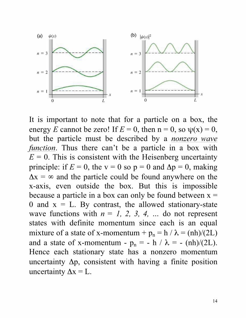
It is important to note that for a particle on a box, the energy E cannot be zero! If E = 0, then n = 0, so ψ(x) = 0, but the particle must be described by a nonzero wave function. Thus there can’t be a particle in a box with E = 0. This is consistent with the Heisenberg uncertainty principle: if E = 0, the v = 0 so p = 0 and Δp = 0, making Δx = ∞ and the particle could be found anywhere on the x-axis, even outside the box. But this is impossible because a particle in a box can only be found between x = 0 and x = L. By contrast, the allowed stationary-state wave functions with n = 1, 2, 3, 4, … do not represent states with definite momentum since each is an equal mixture of a state of x-momentum + pn = h / λ = (nh)/(2L) and a state of x-momentum - pn = - h / λ = - (nh)/(2L). Hence each stationary state has a nonzero momentum uncertainty Δp, consistent with having a finite position uncertainty Δx = L.

15

40.5 The Quantum Mechanical Harmonic Oscillator A harmonic oscillator is a particle of mass m that moves along the x-axis under the influence of a conservative force that obeys Hooke’s law: Fx = - k’ x =- m ω2 x where k’ is the force constant and ω is the angular frequency. The corresponding potential energy function U(x) is

U(x) = 12m! 2 x2

and the one-dimensional time-independent Schrodinger equation becomes:

!!2

2md 2!(x)dx2

+12m" 2x2 !(x) = E!(x)

The solutions to this equation are called Hermite functions, which consist of an exponential function multiplied by a polynomial in x. The quantized energy levels of the quantum mechanical harmonic oscillator are given by

En = !! n+ 12

!

"#

$

%&

16

where the discrete index n is a quantum number that takes on the values n = 0, 1, 2, 3, 4, … Notice that adjacent energy levels are separated by a constant interval of !! = h f, as Max Planck had assumed in 1900. There are infinitely many levels; this should not be surprising because the potential energy function is an infinitely deep potential well.

The normalized wave functions corresponding to the ground state (n = 0) and the first excited state (n = 1) are:

17

!o (x) =m"#!

!

"#

$

%&

14e'm"2

2!"x2

!1(x) =m"#!

!

"#

$

%&

14 2m"!

x e'm"2

2!"x2

18