36

CHAPTER 4

Simulation Results

We use SimReal Inc. NCTUns 1.0 network simulator [16] and simulate on IEEE 802.11b

wireless unslotted, contention-based environment. The MAC protocol of NCTUns is

ported from NS-2 network simulator which implements the complete IEEE 802.11 standard

MAC protocol DCF to accurately model the contention of nodes for the wireless medium.

Here we perform some topologies to simulate several kinds of situation in single-hop,

two-hop and multi-hop to evaluate our proposed path bandwidth calculation scheme. We

compare the error percentage between the estimated (our proposed formula) and real

(according to log files) remaining bandwidth percentage (idle percentage), and see if the

error percentage is acceptable. Section 4.2 shows the topologies we simulate; O1 (or O2,

O3) are the observers which watch the external network traffic load. IS transmits data flow

to ID through UDP/CBR/VBR.

4.1 Parameters

In this section, we set parameters of 802.11 MAC and traffic characteristics. The

following parts list these numerical data.

37

4.1.1 Parameters of IEEE 802.11 MAC

The Table.4.1 lists the parameters of 802.11 MAC protocol we use. Distance between

directly connected stations is within the nominal transmission radius of 250 meters. The

bandwidth is 11 Mbps, and the 100 % of idle percentage is set to be about 5.35 Mbps. We

set RTS Threshold to 0 to perform RTS-CTS before each DATA transmission to eliminate

the cost of transmission fail which is caused by collision and hidden terminal.

Table 4.1: Parameters of IEEE 802.11 MAC.

IEEE 802.11 MAC

aSlotTime 20us

RTS Threshold 0

SIFS 20us

PIFS 30us

DIFS 40us

CWmin 31

CWmax 1023

aShortRetryLimit 7

aLongRetryLimit 4

4.1.2 Traffic Characteristics

We model different traffic loadings in each simulation, CBR and VBR. CBR traffic flows,

with constant packet-generated intervals and constant packet size. And VBR traffic flows,

38

with various packet-generated intervals of exponential distribution and constant packet size.

The Table.4.2 below shows traffic characteristics.

Table 4.2: Traffic Characteristics.

Traffic Characteristics

CBR VBR

Constant Exponential

Interval (msec) 18

Mean 18

Min 9

Max 180

Constant Constant Packet Size (byte)

1472 1472

Mean Rate (Kbps) 86 57

4.1.3 Calculation of each node’s idle percentage

In our simulation, each node could acquire its own idle/busy condition from the MAC layer;

then we can calculate the total idle time from the information. And the idle percentage of

each node is the total idle time divides by total simulation time.

Idle percentage of each node = timesimulationtotalsnode

timeidletotalsnode___'

___'

4.2 Scenarios and Results

We introduce several scenarios which include single-hop, two-hop and multi-hop to evaluate

39

our proposed path bandwidth calculation scheme. Each has several different case study

topologies to represent diverse network mutual relationships. And at last, we model a

typical wireless multi-hop topology to evaluate the performance.

4.2.1 Single Hop

We simulate several single-hop network topologies to evaluate our proposed bandwidth

estimation formula. We change different external traffic load (IS to ID) in each topology;

O1 and O2 are the observers which has no data flow between them.

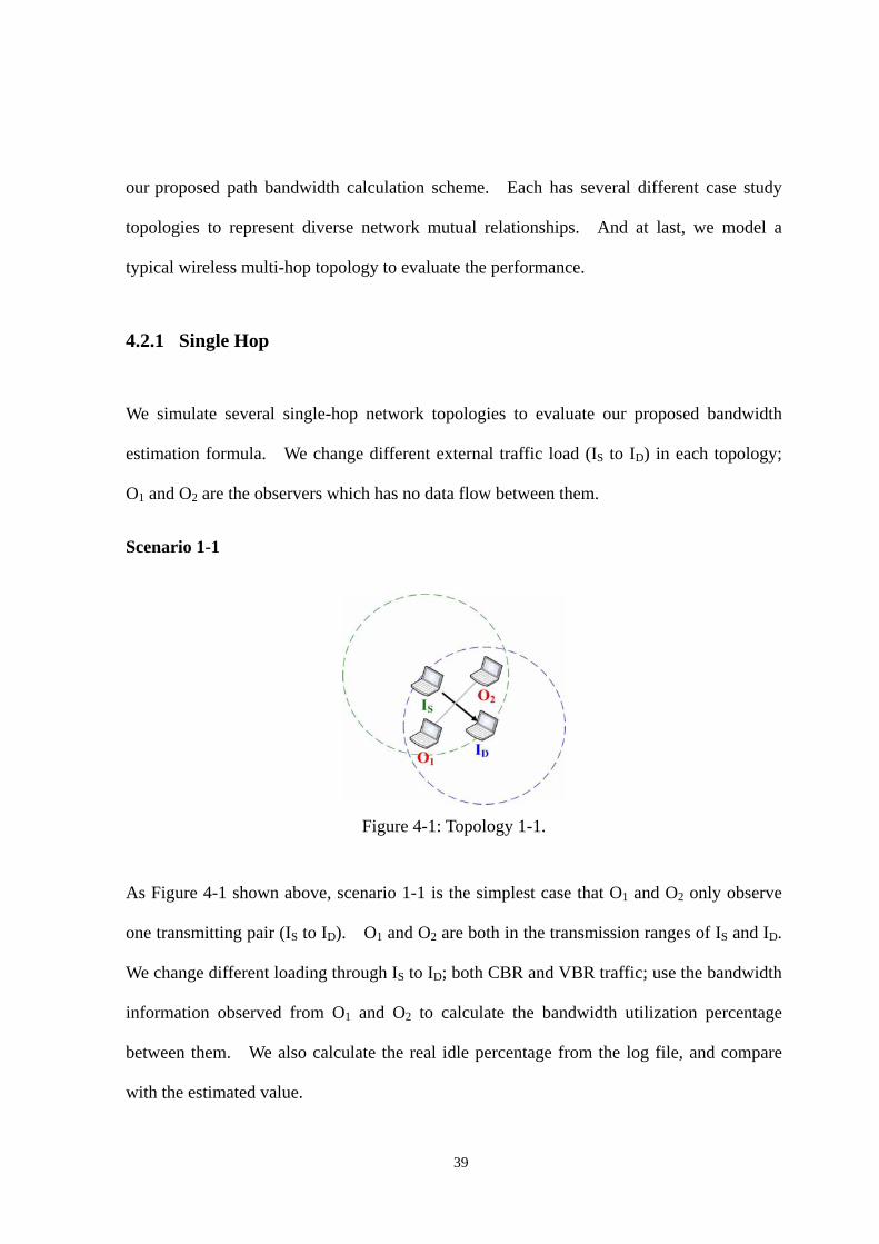
Scenario 1-1

Figure 4-1: Topology 1-1.

As Figure 4-1 shown above, scenario 1-1 is the simplest case that O1 and O2 only observe

one transmitting pair (IS to ID). O1 and O2 are both in the transmission ranges of IS and ID.

We change different loading through IS to ID; both CBR and VBR traffic; use the bandwidth

information observed from O1 and O2 to calculate the bandwidth utilization percentage

between them. We also calculate the real idle percentage from the log file, and compare

with the estimated value.

40

Figure 4-2 shows the comparison of the O1 to O2 link between estimated idle

percentage and the real idle percentage in the single-hop cases.

Figure 4-2: Case 1-1 in Single Hop Topology.

Figure 4-3: Single Hop CBR Throughput.

41

Next, we also add traffic in the observers to verify if the admission control scheme is

feasible by using our path bandwidth calculation scheme. Here we add additionally

different CBR and VBR traffic loading in the original 1-1 scenario.

Figure 4-4: Single Hop VBR Throughput.

Figure 4-5: Available Bandwidth Comparison with CBR/VBR Traffic.

42

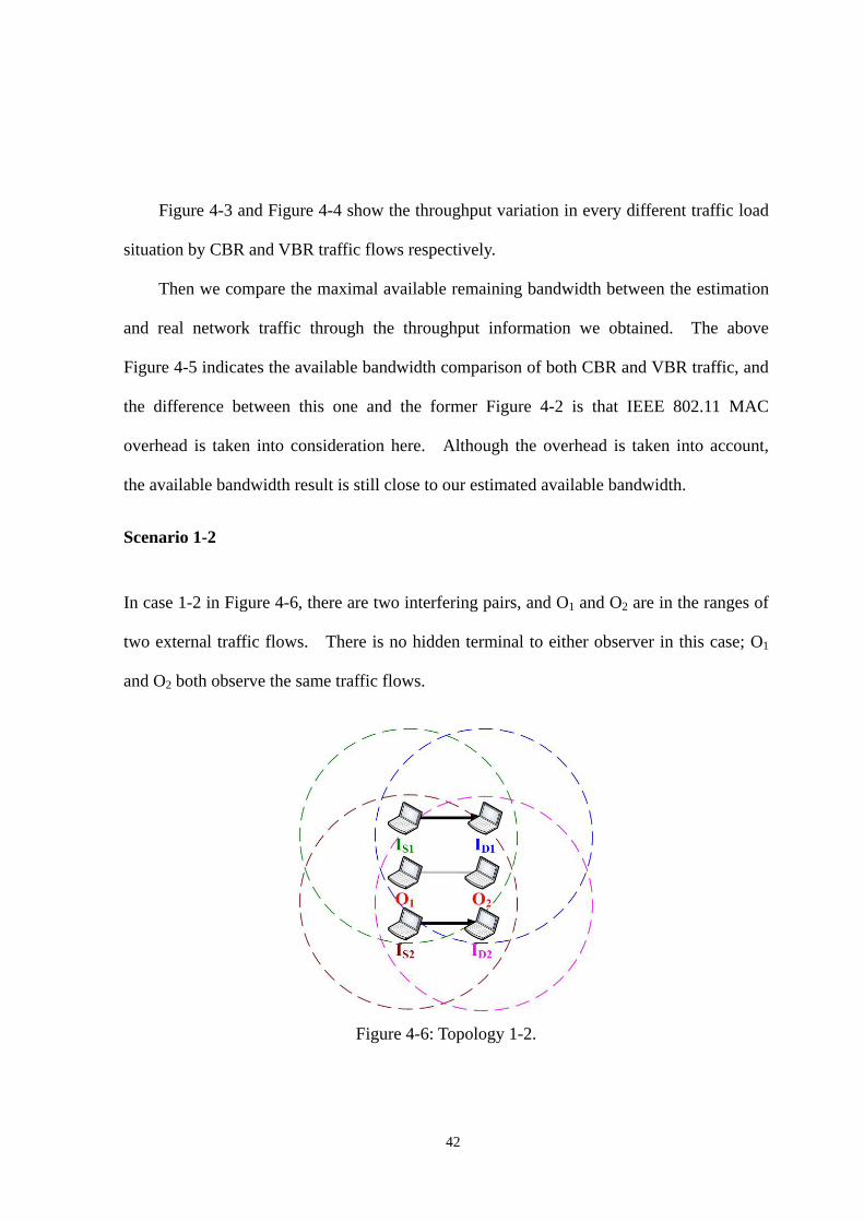
Figure 4-3 and Figure 4-4 show the throughput variation in every different traffic load

situation by CBR and VBR traffic flows respectively.

Then we compare the maximal available remaining bandwidth between the estimation

and real network traffic through the throughput information we obtained. The above

Figure 4-5 indicates the available bandwidth comparison of both CBR and VBR traffic, and

the difference between this one and the former Figure 4-2 is that IEEE 802.11 MAC

overhead is taken into consideration here. Although the overhead is taken into account,

the available bandwidth result is still close to our estimated available bandwidth.

Scenario 1-2

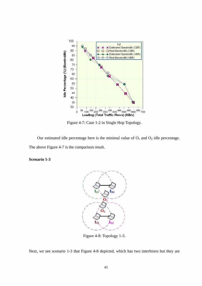
In case 1-2 in Figure 4-6, there are two interfering pairs, and O1 and O2 are in the ranges of

two external traffic flows. There is no hidden terminal to either observer in this case; O1

and O2 both observe the same traffic flows.

Figure 4-6: Topology 1-2.

43

Figure 4-7: Case 1-2 in Single Hop Topology.

Our estimated idle percentage here is the minimal value of O1 and O2 idle percentage.

The above Figure 4-7 is the comparison result.

Scenario 1-3

Figure 4-8: Topology 1-3.

Next, we see scenario 1-3 that Figure 4-8 depicted, which has two interferers but they are

44

totally independent to the two observers O1 and O2. That is, O1 is only affected by IS1 to

ID1, and O2 is only influenced by IS2 to ID2; IS1 and ID1 are the hidden terminals to O2. The

idle percentage between O1 and O2 is the case xy, and Figure 4-9 is the result.

Figure 4-9: Case 1-3 in Single Hop Topology.

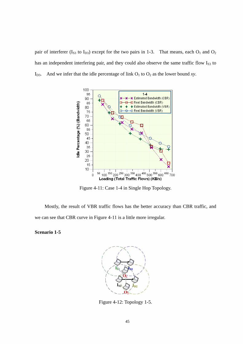
Scenario 1-4

Figure 4-10: Topology 1-4.

Topology 1-4, as Figure 4-10 shown, is a little more complicated than 1-3; we add another

45

pair of interferer (IS3 to ID3) except for the two pairs in 1-3. That means, each O1 and O2

has an independent interfering pair, and they could also observe the same traffic flow IS3 to

ID3. And we infer that the idle percentage of link O1 to O2 as the lower bound xy.

Figure 4-11: Case 1-4 in Single Hop Topology.

Mostly, the result of VBR traffic flows has the better accuracy than CBR traffic, and

we can see that CBR curve in Figure 4-11 is a little more irregular.

Scenario 1-5

Figure 4-12: Topology 1-5.

46

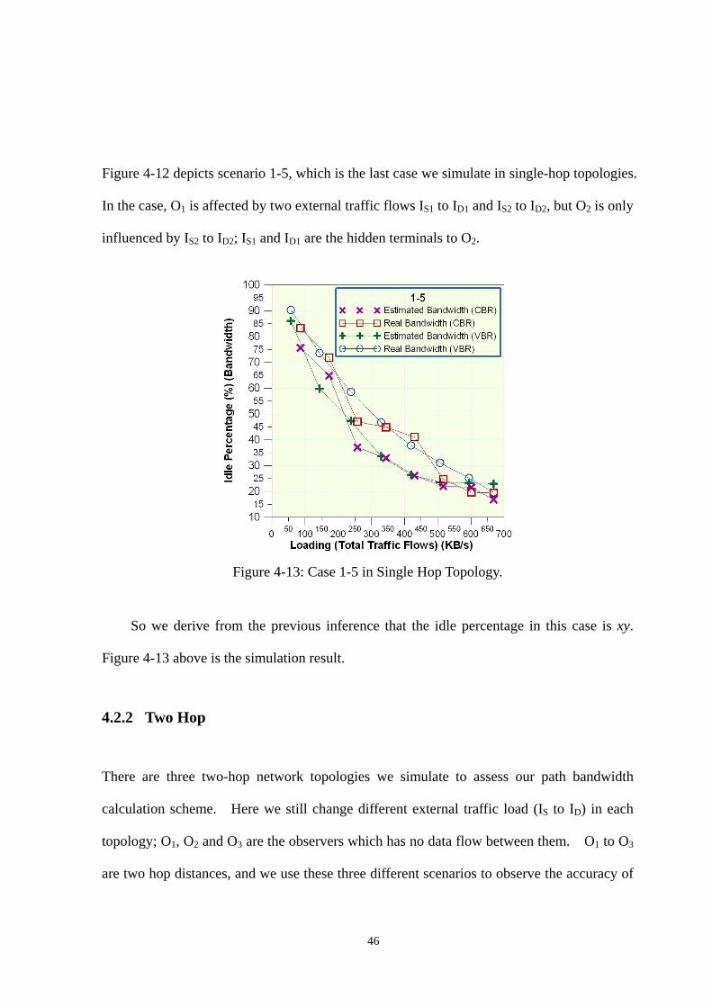
Figure 4-12 depicts scenario 1-5, which is the last case we simulate in single-hop topologies.

In the case, O1 is affected by two external traffic flows IS1 to ID1 and IS2 to ID2, but O2 is only

influenced by IS2 to ID2; IS1 and ID1 are the hidden terminals to O2.

Figure 4-13: Case 1-5 in Single Hop Topology.

So we derive from the previous inference that the idle percentage in this case is xy.

Figure 4-13 above is the simulation result.

4.2.2 Two Hop

There are three two-hop network topologies we simulate to assess our path bandwidth

calculation scheme. Here we still change different external traffic load (IS to ID) in each

topology; O1, O2 and O3 are the observers which has no data flow between them. O1 to O3

are two hop distances, and we use these three different scenarios to observe the accuracy of

47

the estimation in two-hop link.

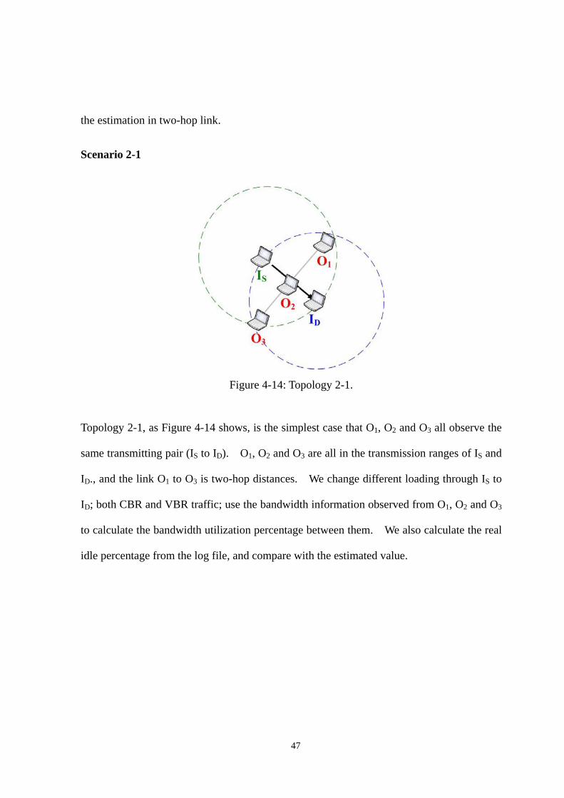
Scenario 2-1

Figure 4-14: Topology 2-1.

Topology 2-1, as Figure 4-14 shows, is the simplest case that O1, O2 and O3 all observe the

same transmitting pair (IS to ID). O1, O2 and O3 are all in the transmission ranges of IS and

ID., and the link O1 to O3 is two-hop distances. We change different loading through IS to

ID; both CBR and VBR traffic; use the bandwidth information observed from O1, O2 and O3

to calculate the bandwidth utilization percentage between them. We also calculate the real

idle percentage from the log file, and compare with the estimated value.

48

Figure 4-15: Case 2-1 in Two Hop Topology.

Figure 4-15 shows the comparison of the O1 to O3 link between estimated idle

percentage and the real idle percentage in the two-hop cases.

Figure 4-16: Two Hop CBR Throughput.

49

Figure 4-17: Two Hop VBR Throughput.

And next, we add different CBR and VBR traffic load (O1 to O3) in the original 2-1

scenario. Figure 4-16 and Figure 4-17 show the throughput variation in every different

traffic load situation of CBR and VBR traffic flows individually.

Figure 4-18: Available Bandwidth Comparison with CBR/VBR Traffic.

50

Then we can compare the maximal available remaining bandwidth between the

estimation and real network traffic through the throughput information we obtained.

Figure 4-18 depicts the comparison of CBR and VBR traffic.

Scenario 2-2

Figure 4-19: Topology 2-2.

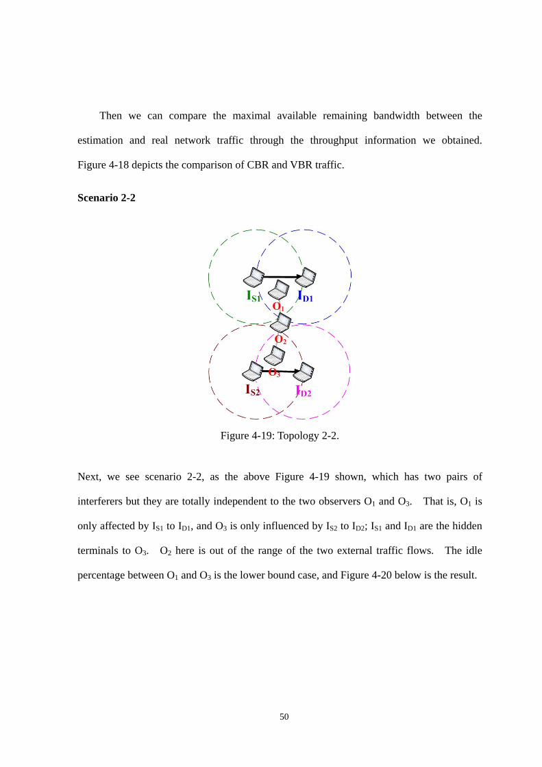
Next, we see scenario 2-2, as the above Figure 4-19 shown, which has two pairs of

interferers but they are totally independent to the two observers O1 and O3. That is, O1 is

only affected by IS1 to ID1, and O3 is only influenced by IS2 to ID2; IS1 and ID1 are the hidden

terminals to O3. O2 here is out of the range of the two external traffic flows. The idle

percentage between O1 and O3 is the lower bound case, and Figure 4-20 below is the result.

51

Figure 4-20: Case 2-2 in Two Hop Topology.

Scenario 2-3

Figure 4-21: Topology 2-3.

Figure 4-21 depicts the scenario 2-3, which is more complicated than scenario 2-2; we add

another pair of interferer (IS3 to ID3) except for the two independent pairs in 2-2. That

means, each O1 and O3 has an independent interfering pair, and they could also observe the

52

same traffic flow IS3 to ID3. And we also infer that the idle percentage of link O1 to O3 as

the lower bound.

Figure 4-22 is the simulation result of case 2-3. We can see that the result of 2-3 has

larger error percentage than all the other scenarios. It might be caused by our calculation

inaccuracy.

Figure 4-22: Case 2-3 in Two Hop Topology.

4.2.3 Multi Hop

There are two multi-hop network topologies we simulate to assess our path bandwidth

calculation scheme. Here we still change different external traffic load (IS to ID) in each

topology; O1, O2, O3 and O4 are the observers which has no data flow between them. Both

O1 to O3 and O2 to O4 are two hop distances, and we use these two different scenarios to

observe the accuracy of the estimation in multi-hop link.

53

Scenario 3-1

Figure 4-23: Topology 3-1.

Case 3-1, as Figure 4-23, O1 is only in the transmission range of IS1 and ID1; O2 and O3 are

out of the transmission ranges of all the interferers, and O4 is in the transmission range of IS2

and ID2. We change different loading through IS1 to ID1 and IS2 to ID2 with both CBR and

VBR traffic. Then we use the bandwidth information observed from O1, O2, O3 and O4 to

calculate the bandwidth utilization percentage between them. We also calculate the real

idle percentage from the log file, and compare with the estimated value.

54

Figure 4-24: Case 3-1 in Multi Hop Topology.

Figure 4-24 shows the comparison of the O1 to O4 link between estimated idle

percentage and the real idle percentage in the multi-hop cases.

Figure 4-25: Multi Hop CBR Throughput.

55

Figure 4-26: Multi Hop VBR Throughput.

And next, we add different CBR and VBR traffic load (O1 to O4) in the original 3-1

scenario. Figure 4-25 and Figure 4-26 show the throughput variation in every different

traffic load situation of CBR and VBR traffic flows individually.

Figure 4-27: Available Bandwidth Comparison with CBR/VBR Traffic.

56

Then we can compare the maximal available remaining bandwidth between the

estimation and real network traffic through the throughput information we obtained.

Figure 4-27 depicts the comparison of CBR and VBR traffic.

Scenario 3-2

The second multi-hop topology is as Figure 4-28, O1 is only in the transmission range of IS1

and ID1; O2 is out of the transmission ranges of all the interferers; O3 is in the transmission

ranges of both IS2 to ID2 and IS3 to ID3, and O4 is only in the transmission range of IS3 and ID3.

We change different loading through IS1 to ID1, IS2 to ID2, and IS3 to ID3; both CBR and VBR

traffic; use the bandwidth information observed from O1, O2, O3 and O4 to calculate the

bandwidth utilization percentage of whole path from O1 to O4 through this topology.

Figure 4-28: Topology 3-2.

We also calculate the real idle percentage from the log file, and compare with the

estimated value. Figure 4-29 below is the result.

57

Figure 4-29: Case 3-2 in Multi Hop Topology.

4.2.4 Integrated Scenario

Figure 4-30: Integrated Topology.

Figure 4-30 shows the topology of typical multi-hop wireless network. Here we fix three

interfering pairs to {F, G}, {C, D} and {E, K} as background traffic and vary the total

58

traffic loads (of the interfering pairs). Then we choose several S/D (Source/Destination)

pairs randomly which might be single-hop, two-hop or multi-hop in different time scales.

Each run, we set the total simulation time to 50 seconds; we select 10 different S/D pairs in

each run and totally 10 runs to calculate the average of the simulation results. Then we

evaluate their efficiency of supporting QoS. We define ATR (Achieved Throughput Ratio)

for S/D pairs as one of the efficiency representation.

ATR = )( andwidthEstimatedBdOfferedLoa

Throughput=

100% of ATR is the perfect situation, which means that we could efficiently use the

available bandwidth as we estimated.

Normalized one-hop average delay performs another efficiency representation.

Because the S/D pair we choose is random, so we normalize the delay time to one-hop

distance delay time and get the average of them.

Figure 4-31: Average Achieved Throughput Ratio.

59

Figure 4-31 is the simulation result which depicts the average achieved throughput

ratio. The ATR decreases slightly in substance while the background traffic loading

increases. Overall, the average ATR are acceptable which are almost above 85 percent.

Because there is a statistical inaccuracy flaw in our solution, it’s almost impossible to

achieve 100 percent bandwidth utilization, which is caused by the calculation error or IEEE

802.11 overhead.

Figure 4-32: Mean Normalized Delay Time.

Figure 4-32 shows the normalized delay time of the simulation. The mean

normalized delay time soars with the increase of traffic load; the VBR traffic delay time

ascends more obvious than CBR traffic delay time when traffic load is high. This result

might be caused by IEEE 802.11 overhead. And when the traffic loading is high, which

means that the remaining bandwidth is small. In such situation, if we estimate the path

60

bandwidth wrong, the influence would be vast, and the delay time would soar apparently.

Our proposed method does support bandwidth guarantee, but it doesn’t ensure the

delay time. So in this simulation, we can see that when traffic loading is high, the

normalized delay time soars obviously, but the guaranteed bandwidth still maintains a

certain level. This might be another point to investigate in the future work.